Quantum State Tomography with Joint SIC POMs and Product SIC POMs

Abstract

We introduce random matrix theory to study the tomographic efficiency of a wide class of measurements constructed out of weighted 2-designs, including symmetric informationally complete (SIC) probability operator measurements (POMs). In particular, we derive analytic formulae for the mean Hilbert-Schmidt distance and the mean trace distance between the estimator and the true state, which clearly show the difference between the scaling behaviors of the two error measures with the dimension of the Hilbert space. We then prove that the product SIC POMs—the multipartite analogue of the SIC POMs—are optimal among all product measurements in the same sense as the SIC POMs are optimal among all joint measurements. We further show that, for bipartite systems, there is only a marginal efficiency advantage of the joint SIC POMs over the product SIC POMs. In marked contrast, for multipartite systems, the efficiency advantage of the joint SIC POMs increases exponentially with the number of parties.

I Introduction

Quantum state tomography is a procedure for inferring the state of a quantum system from generalized measurements. It is a primitive of quantum computation, quantum communication, and quantum cryptography, because all these tasks rely heavily on our ability to determine the state of a quantum system at various stages. One of the main challenges in quantum state tomography is to reconstruct a generic unknown quantum state as efficiently as possible and to determine the resources necessary to achieve a given accuracy, which can be quantified by various figures of merit, such as the trace distance, the Hilbert-Schmidt (HS) distance, or the fidelity ParR04 ; LvoR09 .

A generalized measurement in quantum mechanics is known as a probability operator measurement (POM). A measurement is informationally complete (IC) if any state is determined completely by the measurement statistics Pru77 ; Bus91 ; DarPS04 . In a $d$-dimensional Hilbert space, an IC measurement consists of at least $d^{2}$ outcomes, whereas a minimal IC measurement consists of no more than $d^{2}$ outcomes. A particularly appealing choice of IC measurements are those constructed out of weighted 2-designs, called tight IC measurements according to Scott Sco06 ; RoyS07 . Under linear quantum state tomography, they not only feature a simple state reconstruction formula but also minimize the mean squared error (MSE)— the mean square HS distance between the estimator and the true state Sco06 . The construction of tight IC measurements has also been discussed in detail in Ref. RoyS07 .

A symmetric informationally complete (SIC) POM Zau11 ; RenBSC04 ; App05 ; ScoG10 is a very special tight IC measurement composed of $d^{2}$ subnormalized projectors onto pure states with equal pairwise fidelity of $1/(d+1)$. They may be considered as fiducial measurements for state tomography for reasons of their high symmetry and high tomographic efficiency RenBSC04 ; App05 ; ScoG10 ; RehEK04 ; Sco06 . It is widely believed that SIC POMs exist in any Hilbert space of finite dimension since Zauner posed the conjecture Zau11 , although no rigorous proof is known. Analytical solutions of SIC POMs are known for $d\leq 16$ and $d=19,24,28,35,48$, see Refs. Zau11 ; RenBSC04 ; App05 ; ScoG10 ; Gra11 and the references therein; numerical solutions with high precision have also been found up to $d=67$ RenBSC04 ; RenBSC04b ; ScoG10 . In addition to their significance in quantum state tomography, SIC POMs have attracted much attention due to their connections with mutually unbiased bases (MUB) Iva81 ; WooF89 ; Woo06 ; App09 ; DurEBZ10 , equiangular lines LemS73 , Lie algebras AppFF11 , and foundational studies Fuc10 .

The trace distance is one of the most important distance measures and distinguishability measures in quantum mechanics, and is widely used in quantum state tomography, quantum cryptography, and entanglement theory ParR04 ; NieC00 ; BenZ06 ; FucG99 ; HorHHH09 , as well as other contexts. In addition, it is closely related to other important figures of merit, such as the fidelity and the Shannon distinguishability NieC00 ; FucG99 . However, little is known about the tomographic resources required to achieve a given accuracy as measured by the trace distance, since its definition involves taking the square root of a positive operator. Even for the qubit SIC POM RehEK04 ; LinLK08 ; BurLDG08 , no analytic formula is known concerning the mean trace distance between the estimator and the true state. One motivation of the present study is to solve this long-standing open problem.

In the case of a bipartite or multipartite system, it is technologically much more challenging to perform full joint measurements such as SIC POMs on the whole system. Moreover, in some important realistic scenarios, such as tomographic quantum key distribution LiaKEK03 ; EngKRN04 ; DurKLL08 , all parties are space separated from each other, and it is impractical to perform full joint measurements. Nevertheless, each party can perform a local SIC POM and reconstruct the global state after gathering all the data obtained. Such a POM will henceforth be referred to as a product SIC POM; by contrast, the SIC POM of the whole system will be referred to as a joint SIC POM. The product SIC POM is particularly appealing in tomographic quantum key distribution since it minimizes the redundant information and classical communication required to exchange measurement data among different parties DurKLL08 . However, even less is known concerning the tomographic efficiency of the product SIC POM except for numerical studies in the two-qubit setting BurLDG08 ; TeoZE10 .

In this article, we aim at characterizing the tomographic efficiency of tight IC measurements in terms of the mean trace distance and the mean HS distance, with special emphasis on the minimal tight IC measurements—SIC POMs. We also determine the efficiency gap between the product measurements and the joint measurements in the bipartite and multipartite settings.

First, we introduce random matrix theory Meh04 to study the tomographic efficiency of tight IC measurements and derive analytical formulae for the mean trace distance and the mean HS distance. We illustrate the general result with SIC POMs, and show the different scaling behaviors of the two error measures with the dimension of the Hilbert space. In the special case of the qubit SIC POM, we discuss in detail the dependence of the reconstruction error on the Bloch vector of the unknown true state and make contact with the experimental data given by Ling et al. LinLK08 . As a by product, we also discovered a special class of tight IC measurements that feature exceptionally symmetric outcome statistics and low fluctuation over repeated experiments.

Second, in the bipartite and multipartite settings, we show that the product SIC POMs are optimal among all product measurements in the same sense as the joint SIC POMs are optimal among all joint measurements. We further show that for bipartite systems, there is only a marginal efficiency advantage of the joint SIC POMs over the product SIC POMs. Hence, it is not worth the trouble to perform the joint measurements. However, for multipartite systems, the efficiency advantage of the joint SIC POMs increases exponentially with the number of parties.

To provide a simple picture of the tomographic efficiency of SIC POMs and product SIC POMs, we restrict our attention to the scenario where the number of copies of the true states available is large enough to yield a reasonably good estimator, and we focus on the standard state reconstruction scheme, also known as linear state tomography ParR04 ; Sco06 . The analysis of the efficiencies of other reconstruction schemes, such as the maximum likelihood method ParR04 ; Hra97 ; TeoZE10 , is much more involved. Hopefully, our analysis can serve as a starting point and, in principle, it can be generalized to deal with those more complicated situations. Moreover, for minimal tomography on a large sample, the estimator given by the standard reconstruction scheme is almost identical to that given by the maximum-likelihood method, except when the true state is very close to the boundary of the state space. Hence, the efficiencies of the two alternative schemes are quite close to each other in this scenario.

The rest of this article is organized as follows. In Sec. II, we review the basic framework for linear state tomography and recall the concepts of weighted $t$-designs, SIC POMs and tight IC measurements. In Sec. III, we introduce random matrix theory to study the tomographic efficiency of tight IC measurements, in particular the SIC POMs. We derive analytical formulae for the mean trace distance and the mean HS distance and illustrate the difference in their scaling behaviors with the dimension of the Hilbert space. In Sec. IV, we first prove the optimality of the product SIC POMs among product measurements and then compare the tomographic efficiencies of the product SIC POMs and the joint SIC POMs. We conclude with a summary.

II Setting the stage

II.1 Linear state tomography

A generalized measurement is composed of a set of outcomes represented mathematically by positive operators $\Pi_{j}$ that sum up to the identity operator 1. Given an unknown true state $\rho$, the probability of obtaining the outcome $\Pi_{j}$ is given by the Born rule: $p_{j}=\mathrm{tr}(\Pi_{j}\rho)$. A measurement is IC if we can reconstruct any state according to the statistics of measurement results, that is the set of probabilities $p_{j}$. If we take both the state $\rho$ and the outcomes $\Pi_{j}$ as vectors in the space of Hermitian operators, then the probability can be expressed as an inner product $\langle\!\langle\Pi_{j}|\rho\rangle\!\rangle\equiv\mathrm{tr}(\Pi_{j}\rho)$, where we have borrowed the double ket (bra) notation from Refs. DarPS00 ; DarP07 . Furthermore, an out product such as $|\Pi_{j}\rangle\!\rangle\langle\!\langle\Pi_{j}|$, which is referred to as an superoperator henceforth, acts on this space just as an operator acts on the ordinary Hilbert space (the arithmetics of superoperators can be found in Refs. RunMND00 ; RunBCH01 ). With this background, one can show that a measurement is IC if and only if the frame superoperator

$$\mathcal{F}=\sum_{j}\frac{|\Pi_{j}\rangle\!\rangle\langle\!\langle\Pi_{j}|}{\mathrm{tr}(\Pi_{j})}$$ (1)

is invertible Sco06 ; DufS52 ; Cas00 ; DarP07 . The frame superoperator $\mathcal{F}$ can be written in the following form Sco06

$$\mathcal{F}=\frac{\mathcal{I}}{d}+\mathcal{F}_{0},$$ (2)

where $\mathcal{I}=|1\rangle\!\rangle\langle\!\langle 1|$ and

$$\mathcal{F}_{0}=\sum_{j}\frac{|\Pi_{j}-\mathrm{tr}(\Pi_{j})/d\rangle\!\rangle\langle\!\langle\Pi_{j}-\mathrm{tr}(\Pi_{j})/d|}{\mathrm{tr}(\Pi_{j})},$$ (3)

which is supported on the space of traceless Hermitian operators. Obviously, $\mathcal{F}$ is invertible if and only if $\mathcal{F}_{0}$ is invertible in this space. In the rest of this article, $\mathcal{F}_{0}$ will also be referred to as the frame superoperator if there is no confusion.

When $\mathcal{F}$ is invertible, there exists a set of reconstruction operators $\Theta_{j}$ satisfying $\sum_{j}|\Theta_{j}\rangle\!\rangle\langle\!\langle\Pi_{j}|=\mathbf{I}$, where $\mathbf{I}$ is the identity superoperator. Given a set of reconstruction operators, any state can be reconstructed from the set of probabilities $p_{j}$: $\rho=\sum_{j}p_{j}\Theta_{j}$. In a realistic scenario, given $N$ copies of the unknown true state, what we really get in an experiment are frequencies $f_{j}$ rather than probabilities $p_{j}$. The estimator based on these frequencies $\hat{\rho}=\sum_{j}f_{j}\Theta_{j}$ is thus different from the true state. Nevertheless, the deviation $\Delta\rho=\hat{\rho}-\rho$ vanishes in the large-$N$ limit if the measurement is IC. In general, these frequencies obey a multinomial distribution with the MSE matrix (also called the covariance matrix) $\Sigma_{jk}=\bigl{(}p_{j}\delta_{jk}-p_{j}p_{k}\bigr{)}/N$. The MSE matrix of the estimator $\hat{\rho}$ can be derived according to the principle of error propagation,

$$\mathcal{C}(\rho) = \sum_{j,k}|\Theta_{j}\rangle\!\rangle\Sigma_{jk}\langle\!\langle\Theta_{k}|$$ (4)

$$= \frac{1}{N}\biggl{(}\sum_{j}|\Theta_{j}\rangle\!\rangle\langle\!\langle\Pi_{j}|\rho\rangle\!\rangle\langle\!\langle\Theta_{j}|-|\rho\rangle\!\rangle\langle\!\langle\rho|\biggr{)}.$$

The MSE is exactly the trace of the MSE matrix,

$$\mathcal{E}_{\mathrm{M}}(\rho) \equiv \mathrm{E}(|\!|\Delta\rho|\!|^{2}_{\mathrm{HS}})=\mathrm{Tr}(\mathcal{C}(\rho))$$ (5)

$$= \frac{1}{N}\biggl{(}\sum_{j}p_{j}\mathrm{tr}\bigl{(}\Theta_{j}^{2}\bigr{)}-\mathrm{tr}(\rho^{2})\biggr{)}.$$

In this article, the symbol “$\mathrm{Tr}$” is used to denote the trace for superoperators, and “$\mathrm{tr}$” that for ordinary operators. For the convenience of later discussions, we define $N\mathcal{E}_{\mathrm{M}}(\rho)$ as the scaled MSE, which is independent of $N$. The scaled mean trace distance and the scaled mean HS distance can be defined similarly, except that $N$ is replaced by $\sqrt{N}$.

The set of reconstruction operators is unique for a minimal IC measurement, such as a SIC POM or a product SIC POM, but is not unique for a generic IC measurement. Among all the candidates, the set of canonical reconstruction operators

$$|\Theta_{j}\rangle\!\rangle=\frac{\mathcal{F}^{-1}|\Pi_{j}\rangle\!\rangle}{\mathrm{tr}(\Pi_{j})}$$ (6)

is the best choice for linear state reconstruction in that it minimizes the MSE averaged over unitarily equivalent true states and is thus widely used in practice Sco06 . In the rest of this article, we will only consider canonical reconstruction operators. It is then straightforward to verify that $|1\rangle\!\rangle$ is an eigenvector of $\mathcal{C}(\rho)$ with eigenvalue $0$; in other words, $\mathcal{C}(\rho)$ is supported on the space of traceless Hermitian operators as is $\mathcal{F}_{0}$. The other eigenvalues of $\mathcal{C}(\rho)$ determine the variances along the principle axes and thus the shape of the uncertainty ellipsoid.

If $N$ is sufficiently large, the multinomial distribution approximates a Gaussian distribution, which is completely determined by the mean and the MSE matrix. In practice, the Gaussian approximation is already quite good for moderate values of $N$ if we are mainly concerned with quantities like the mean HS distance and the mean trace distance, which are the most common figures of merit in quantum state tomography. We thus assume the validity of this approximation in the following discussion. Under Gaussian approximation, the variance of the squared error $|\!|\Delta\rho|\!|^{2}_{\mathrm{HS}}$ is given by the following simple formula:

$$v(\rho)\equiv\mathrm{Var}(|\!|\Delta\rho|\!|^{2}_{\mathrm{HS}})=2\mathrm{Tr}\bigl{(}\mathcal{C}(\rho)^{2}\bigr{)}.$$ (7)

In practice, $\sqrt{v(\rho)}$ quantifies the amount of fluctuation in the squared error $|\!|\Delta\rho|\!|^{2}_{\mathrm{HS}}$ over repeated experiments, that is the typical error in estimating $\mathcal{E}_{\mathrm{M}}(\rho)$ with just one experiment, assuming the true state is known. This error can be reduced by a factor of $\sqrt{N_{\mathrm{e}}}$ if we repeat the experiment $N_{\mathrm{e}}$ times and take the average of $|\!|\Delta\rho|\!|^{2}_{\mathrm{HS}}$. In addition, once $\mathcal{E}_{\mathrm{M}}(\rho)$ is fixed, $v(\rho)$ also quantifies the dispersion of the eigenvalues of $\mathcal{C}(\rho)$, that is the degree of anisotropy in the distribution of the estimators.

II.2 Weighted $t$-designs and SIC POMs

Consider a weighted set of states $\{|\psi_{j}\rangle,w_{j}\}$ with $0<w_{j}\leq 1$ and $\sum_{j}w_{j}=d$, then the order-$t$ frame potential $\Phi_{t}$ for a positive integer $t$ is defined as Sco06 ; RenBSC04

$$\Phi_{t} = \sum_{j,k}w_{j}w_{k}|\langle\psi_{j}|\psi_{k}\rangle|^{2t}=\mathrm{tr}(S_{t}^{2}),$$

$$S_{t} = \sum_{j}w_{j}(|\psi_{j}\rangle\langle\psi_{j}|)^{\otimes t}.$$ (8)

Note that $S_{t}$ is supported on the $t$-partite symmetric subspace, whose dimension is ${d+t-1\choose t}$, $\Phi_{t}$ is bounded from below by $d^{2}{d+t-1\choose t}^{-1}$ and the bound is saturated if and only if $S_{t}=d{d+t-1\choose t}^{-1}P^{\mathrm{sym}}_{t}$, where $P^{\mathrm{sym}}_{t}$ is the projector onto the $t$-partite symmetric subspace. The weighted set $\{|\psi_{j}\rangle,w_{j}\}$ is a (complex projective) weighted $t$-design if the lower bound is saturated; it is a $t$-design if in addition all the weights $w_{j}$ are equal Sco06 ; RenBSC04 . According to the definition, a weighted $t$-design is also a weighted $t^{\prime}$-design for $t^{\prime}<t$.

It is known that for any positive integers $d$ and $t$, there exists a (weighted) $t$-design with a finite number of elements SeyZ84 . However, the number is bounded from below by Hog82 ; Sco06

$${d+\lceil t/2\rceil-1\choose\lceil t/2\rceil}{d+\lfloor t/2\rfloor-1\choose\lfloor t/2\rfloor},$$ (9)

which is equal to $d,d^{2},d^{2}(d+1)/2$ for $t=1,2,3$, respectively. Any resolution of the identity consisting of pure states is a weighted 1-design. SIC POMs Zau11 ; RenBSC04 ; ScoG10 and complete sets of MUB Iva81 ; WooF89 ; DurEBZ10 are prominent examples of 2-designs. The complete set of MUB for $d=2$ is also a 3-design.

A SIC POM is composed of $d^{2}$ subnormalized projectors onto pure states $\Pi_{j}=|\psi_{j}\rangle\langle\psi_{j}|/d$ with equal pairwise fidelity Zau11 ; RenBSC04 ; App05 ; ScoG10 , that is,

$$|\langle\psi_{j}|\psi_{k}\rangle|^{2}=\frac{d\delta_{jk}+1}{d+1},\quad j,k=1,2\cdots,d^{2}.$$ (10)

It is straightforward to verify that a SIC POM is a 2-design from this definition. What is not so obvious is that a weighted 2-design consisting of $d^{2}$ elements must be a SIC POM Sco06 .

A SIC POM is group covariant if it can be generated from a single state—the fiducial state—under the action of a group consisting of unitary operators. Most known SIC POMs are covariant with respect to the Heisenberg–Weyl group (also called the generalized Pauli group) Zau11 ; RenBSC04 ; App05 ; ScoG10 , which is generated by the phase operator $Z$ and the cyclic shift operator $X$ defined by their actions on the computational basis,

$$Z|e_{r}\rangle = \omega^{r}|e_{r}\rangle,$$

$$X|e_{r}\rangle = \left\{\begin{array}[]{cl}|e_{r+1}\rangle&\quad\mbox{if}\;r=0,1,\cdots,d-2,\\ |e_{0}\rangle&\quad\mbox{if}\;r=d-1,\\ \end{array}\right.$$ (13)

where $\omega=e^{2\pi\mathrm{i}/d}$. A fiducial ket $|\psi\rangle$ of the Heisenberg-Weyl group satisfies

$$|\langle\psi|X^{k_{1}}Z^{k_{2}}|\psi\rangle|=\frac{1}{\sqrt{d+1}}$$ (14)

for $k_{1},k_{2}=0,1,\ldots,d-1$ and $(k_{1},k_{2})\neq(0,0)$. Up to now, analytical fiducial kets of the Heisenberg-Weyl group are known for $d\leq 16$ and $d=19,24,28,35,48$ Zau11 ; RenBSC04 ; App05 ; ScoG10 ; Gra11 , numerical fiducial kets with high precision have been found up to $d=67$ RenBSC04 ; RenBSC04b ; ScoG10 .

In this article, all SIC POMs used in the numerical simulation are generated by the Heisenberg-Weyl group from the fiducial kets of Ref. RenBSC04b . However, all theoretical analysis is independent of the specific choice of SIC POMs.

II.3 Tight IC measurements

An IC measurement is tight if the frame superoperator $\mathcal{F}_{0}$ is proportional to $\mathbf{I}_{0}$, that is $\mathcal{F}_{0}=a\mathbf{I}_{0}$ for $a>0$, where $\mathbf{I}_{0}$ is the identity superoperator in the space of traceless Hermitian operators. Scott Sco06 has shown that the coefficient $a$ is upper bounded by $1/(d+1)$ for any tight IC measurement, and the upper bound is saturated if and only if the tight IC measurement is rank one. He also showed that rank-one tight IC measurements are optimal for linear state tomography in the sense that the MSE $\mathcal{E}_{\mathrm{M}}(\rho)$ averaged over unitarily equivalent density operators is minimized Sco06 . Here we shall recapitulate his main idea in a way that suits our subsequent discussion.

Since the average of $\rho$ over unitarily equivalent states is the completely mixed state, according to Eqs. (4) and (5), it is enough to show the optimality of the rank-one tight IC measurements when the true state is the completely mixed state. In that case, the MSE matrix and the MSE can be expressed more concisely in terms of the frame superoperator $\mathcal{F}_{0}$,

$$\mathcal{C}\Bigl{(}\frac{1}{d}\Bigr{)} = \frac{1}{N}\Bigl{(}\frac{\mathcal{F}^{-1}}{d}-\frac{\mathcal{I}}{d^{2}}\Bigr{)}=\frac{1}{dN}\mathcal{F}_{0}^{-1},$$

$$\mathcal{E}_{\mathrm{M}}\Bigl{(}\frac{1}{d}\Bigr{)} = \frac{1}{dN}\mathrm{Tr}\bigl{(}\mathcal{F}_{0}^{-1}\bigr{)}.$$ (15)

The first equation endows the frame superoperator $\mathcal{F}_{0}$ with a concrete operational meaning as the inverse of the MSE matrix (up to a multiplicative factor) evaluated at the point $\rho=1/d$. From the definitions of the frame superoperators $\mathcal{F}$ and $\mathcal{F}_{0}$ (cf. Sec. II.1), we have

$$\mathrm{Tr}(\mathcal{F}_{0})=\mathrm{Tr}(\mathcal{F})-1\leq\sum_{j}\mathrm{tr}(\Pi_{j})-1=d-1,$$ (16)

and the inequality is saturated if and only if the measurement is rank one. Recalling that $\mathcal{F}_{0}$ is supported on the space of traceless Hermitian operators, whose dimension is $d^{2}-1$, the above equation implies that

$$\mathrm{Tr}\bigl{(}\mathcal{F}_{0}^{-1}\bigr{)} \geq (d+1)(d^{2}-1),$$

$$\mathcal{E}_{\mathrm{M}}\Bigl{(}\frac{1}{d}\Bigr{)} \geq \frac{1}{dN}(d+1)(d^{2}-1).$$ (17)

The inequalities are saturated if and only if $\mathcal{F}_{0}=\mathbf{I}_{0}/(d+1)$. In other words, rank-one tight IC measurements are optimal in minimizing the MSE Sco06 .

A rank-one tight IC measurement with outcomes $\Pi_{j}=|\psi_{j}\rangle w_{j}\langle\psi_{j}|$ features particularly simple canonical reconstruction operators

$$\Theta_{j}=|\psi_{j}\rangle(d+1)\langle\psi_{j}|-1$$ (18)

and easy state reconstruction. According to Eq. (5), the MSE is also given by a simple formula Sco06

$$\mathcal{E}_{\mathrm{M}}(\rho)=\frac{1}{N}[d^{2}+d-1-\mathrm{tr}(\rho^{2})],$$ (19)

which is invariant under unitary transformations of the true state. In addition, the MSE matrix evaluated at $\rho=1/d$ is proportional to $\mathbf{I}_{0}$, which means that the uncertainty ellipsoid is isotropic in the space of traceless Hermitian operators. This feature will play a crucial role in our later discussions.

There is a close relation between rank-one tight IC measurements and weighted 2-designs: A rank-one measurement with outcomes $\Pi_{j}=|\psi_{j}\rangle w_{j}\langle\psi_{j}|$ is tight IC if and only if the weighted set $\{|\psi_{j}\rangle,w_{j}\}$ forms a weighted 2-design Sco06 . For example, SIC POMs and complete sets of MUB are rank-one tight IC measurements according to this relation, which can also be verified directly. Hence, Eqs. (18) and (19) are applicable to them. More examples of tight IC measurements can be found in Ref. RoyS07 .

III Applications of random matrix theory to quantum state tomography

In this section, we apply random matrix theory to studying the tomographic efficiency of tight IC measurements and illustrate the general result with SIC POMs. In particular we derive analytical formulae for the mean trace distance and the mean HS distance between the estimator and the true state, thus giving a simple picture of the resources required to achieve a given accuracy as quantified by either of the two distances. Our study also clearly shows the different scaling behaviors of the two error measures with the dimension of the Hilbert space. The idea of computing the mean trace distance using the random matrix theory may also be extended to derive other figures of merit which only depend on the deviation between the estimator and the true state.

The rest of this section is organized as follows. In Sec. III.1, we present the simple idea of computing the mean trace distance and the mean HS distance with random matrix theory. In Sec. III.2, we single out those measurements for which the method is best justified. In Sec. III.3, we show that the method works very well for typical rank-one tight IC measurements, especially SIC POMs. In Sec. III.4, we focus on the qubit SIC POM.

III.1 A simple idea

Here is the simple idea of computing the mean trace distance with random matrix theory: In each experiment, after measurements on $N$ copies of the unknown true state $\rho$, we can construct an estimator $\hat{\rho}$ for the true state according to the procedure described in Sec. II.1. Once a basis is fixed, the deviation $\Delta\rho=\hat{\rho}-\rho$ can be represented by a $d\times d$ matrix, which varies from one experiment to another. After a large number of repeated experiments, the set of matrices $\Delta\rho$ can be taken as an ensemble of random matrices obeying a multidimensional Gaussian distribution, which is completely determined by the MSE matrix $\mathcal{C}(\rho)$,

$$p(\Delta\rho) \propto \exp\Bigl{(}-\frac{1}{2}\langle\!\langle\Delta\rho|\mathcal{C}(\rho)^{-1}|\Delta\rho\rangle\!\rangle\Bigr{)}.$$ (20)

Since $\mathcal{C}(\rho)$ is supported on the space of traceless Hermitian operators, the distribution of $\Delta\rho$ is restricted on the hyperplane satisfying $\mathrm{tr}(\Delta\rho)=0$. Suppose $f(x)$ is the level density function of this ensemble of matrices with normalization convention $\int\mathrm{d}xf(x)=d$. Then the mean trace distance between the estimator and the true state is proportional to the first absolute moment of $f(x)$,

$$\mathcal{E}_{\mathrm{tr}}(\rho)\equiv\frac{1}{2}\mathrm{E}(\mathrm{tr}|\Delta\rho|)=\frac{1}{2}\int\mathrm{d}x\,|x|f(x).$$ (21)

If $\mathcal{C}(\rho)$ is (approximately) proportional to the identity superoperator $\mathbf{I}$, then the ensemble of matrices $\Delta\rho^{\prime}=\sqrt{d^{2}/2\mathcal{E}_{\mathrm{M}}(\rho)}\Delta\rho$ is (approximately) a standard Gaussian unitary ensemble. According to random matrix theory, for sufficiently large $d$, the level density $f_{\mathrm{G}}(x)$ of the Gaussian unitary ensemble is given by the famous Wigner semicircle law Meh04 :

$$f_{\mathrm{G}}(x)=\left\{\begin{array}[]{cl}\frac{1}{\pi}(2d-x^{2})^{1/2}&\quad\mbox{if}\;-\sqrt{2d}\leq x\leq\sqrt{2d},\\ 0&\quad\textrm{otherwise}.\end{array}\right.$$ (24)

We can derive $f(x)$ from $f_{\mathrm{G}}(x)$ by a scale transformation and then compute the mean trace distance between the estimator and the true state, with the outcome

$$\mathcal{E}_{\mathrm{tr}}(\rho) \approx \frac{4}{3\pi}\sqrt{d\mathcal{E}_{\mathrm{M}}(\rho)}.$$ (25)

Furthermore, one can verify that the equation is still quite accurate if $\mathcal{C}(\rho)$ is approximately proportional to $\mathbf{I}_{0}$ instead of $\mathbf{I}$, especially when $d$ is large. In other words, the feasibility of our approach is not limited by the fact that $\mathcal{C}(\rho)$ is supported on the space of traceless Hermitian operators.

When $\mathcal{C}(\rho)$ is proportional to $\mathbf{I}_{0}$, $\Delta\rho$ follows a ($d^{2}-1$)-dimensional isotropic Gaussian distribution and $|\!|\Delta\rho|\!|_{\mathrm{HS}}^{2}$ obeys $\chi^{2}$ distribution with $d^{2}-1$ degree of freedom. The mean HS distance can thus be computed with the result

$$\mathcal{E}_{\mathrm{HS}}(\rho) \equiv \mathrm{E}\Bigl{(}\sqrt{|\!|\Delta\rho|\!|^{2}_{\mathrm{HS}}}\,\Bigr{)}=\sqrt{\frac{\mathcal{E}_{\mathrm{M}}(\rho)}{d^{2}-1}}\frac{\sqrt{2}\Gamma\bigl{(}\frac{d^{2}}{2}\bigr{)}}{\Gamma\bigl{(}\frac{d^{2}-1}{2}\bigr{)}}.$$ (26)

As a consequence of the law of large numbers, when $d$ is large, $\mathcal{E}_{\mathrm{HS}}(\rho)$ is approximately equal to the square root of $\mathcal{E}_{\mathrm{M}}(\rho)$, and with a high probability the estimator $\hat{\rho}$ is distributed within a thin spherical shell of radius $\mathcal{E}_{\mathrm{HS}}(\rho)$ that is centered at the true state.

In general, the accuracy of Eqs. (25) and (26) may depend on the dimension of the Hilbert space and the degree of anisotropy of the uncertainty ellipsoid as determined by $\mathcal{C}(\rho)$. However, it turns out that the mean trace distance and the mean HS distance are not so sensitive to the degree of anisotropy of the uncertainty ellipsoid. As we shall see shortly, the two equations are surprisingly accurate for a large family of measurements, especially tight IC measurements, even if $d$ is very small (see Fig. 1).

Although we have started our analysis with linear state tomography, the idea of computing the mean trace distance with random matrix theory has a wider applicability. We may apply the approach to study the tomographic efficiencies of other reconstruction schemes, such as the maximum-likelihood method. In addition, we may also consider other figures of merit which only depend on the deviation between the estimator and the true state.

III.2 Isotropic measurements

In this section we single out those rank-one IC measurements for which the uncertainty ellipsoid is the most isotropic, in which case Eqs. (25) and (26) are best justified. These measurements turn out to be a special class of tight IC measurements. In addition to minimizing the MSE, they also minimize the fluctuation of reconstruction error over repeated experiments. Moreover, these IC measurements have the nice property that the mean reconstruction error is almost independent of the true state.

When the true state is the completely mixed state, according to Sec. II.3, $\mathcal{C}(1/d)$ is proportional to $\mathbf{I}_{0}$ if and only if the measurement is tight IC, and the coefficient of proportionality is minimized when the measurement is rank-one. The symmetry requirement on the MSE matrix is thus consistent with the efficiency requirement, recall that rank-one tight IC measurements are optimal for linear state tomography. Let us focus on the MSE matrix $\mathcal{C}(\rho)$ for a generic true state, assuming that we have a rank-one tight IC measurement with outcomes $\Pi_{j}=|\psi_{j}\rangle w_{j}\langle\psi_{j}|$. The degree of anisotropy can be quantified by $\overline{\mathrm{Tr}\bigl{(}\mathcal{C}(\rho)^{2}\bigr{)}}-\overline{[\mathrm{Tr}(\mathcal{C}(\rho))]^{2}}$, where the over-line means taking the average over unitarily equivalent density operators. Since $\mathrm{Tr}(\mathcal{C}(\rho))$ is exactly the MSE, which is the same for all rank-one tight IC measurements according to Eq. (19), it suffices to consider $\overline{\mathrm{Tr}\bigl{(}\mathcal{C}(\rho)^{2}\bigr{)}}$. Note that $\overline{\mathrm{Tr}\bigl{(}\mathcal{C}(\rho)^{2}\bigr{)}}$ also quantifies the fluctuation in $|\!|\Delta\rho|\!|^{2}_{\mathrm{HS}}$ over repeated experiments according to Eq. (7). We find

$$N^{2}\overline{\mathrm{Tr}\bigl{(}\mathcal{C}(\rho)^{2}\bigr{)}}=d^{2}+2d-\frac{2}{d}+\bigl{[}\mathrm{tr}(\rho^{2})\bigr{]}^{2}$$

$$\quad{}+\frac{(d+1)^{3}\Phi_{3}-2(2d^{2}+3d-1)}{(d-1)}\Bigl{[}\mathrm{tr}(\rho^{2})-\frac{1}{d}\Bigl{]}$$

$$\quad{}-2\Bigl{[}\frac{2(d+1)}{d+2}\mathrm{tr}(\rho^{3})+\frac{d-1}{d+2}\mathrm{tr}(\rho^{2})-\frac{1}{d+2}\Bigr{]}$$ (27)

$$\geq d^{2}+2d-\frac{2}{d}+2\frac{d^{2}-2}{d+2}\Bigl{[}\mathrm{tr}(\rho^{2})-\frac{1}{d}\Bigl{]}+\bigl{[}\mathrm{tr}(\rho^{2})\bigr{]}^{2}$$

$$\quad{}-2\Bigl{[}\frac{2(d+1)}{d+2}\mathrm{tr}(\rho^{3})+\frac{d-1}{d+2}\mathrm{tr}(\rho^{2})-\frac{1}{d+2}\Bigr{]},\quad$$ (28)

where $\Phi_{3}$ is the order-3 frame potential defined in Eq. (II.2), and we have used the inequality $\Phi_{3}\geq 6d/(d+1)(d+2)$ in deriving Eq. (28). The lower bound is saturated if and only if $\Phi_{3}=6d/(d+1)(d+2)$, that is, when the weighted set $\{|\psi_{j}\rangle,w_{j}\}$ forms a weighted 3-design.

An IC measurement derived from a weighted 3-design will be called an isotropic measurement for reasons that will become clear shortly. By virtue of the properties of weighted $3$-designs, one can show that the MSE matrix $\mathcal{C}(\rho)$ is the same for any IC measurement derived from a weighted 3-design, including the covariant measurement composed of all pure states weighted by the Haar measure. In other words, $\mathcal{C}(\rho)$ is invariant under any unitary transformation of the measurement outcomes: $\Pi_{j}\rightarrow U\Pi_{j}U^{\dagger}$. As an immediate consequence, the reconstruction error is the same for unitarily equivalent true states as long as the figure of merit is unitarily invariant, such as the mean trace distance, the mean HS distance, or the mean fidelity.

Under linear state tomography, in addition to achieving the minimal MSE $\mathcal{E}_{\mathrm{M}}(\rho)$, an isotropic measurement also minimizes the fluctuation of the statistical error over repeated experiments, or equivalently the degree of anisotropy in the distribution of $\Delta\rho$. One can show that with an isotropic measurement, $N\mathcal{C}(\rho)$ for a pure true state has only four (three if $d=2$) distinct eigenvalues, $(d+1)/(d+2),2(d+1)/(d+2),0,2d/(d+2)$ with multiplicities $d(d-2),2(d-1),1,1$, respectively. The degree of anisotropy is even lower if the true state has a lower purity since the leading term in the expression of $\mathcal{C}(\rho)$ [cf. Eq. (4)] is linear in $\rho$.

In conclusion, Eqs. (25) and (26) are a good approximation for computing the mean trace distance and the mean HS distance under isotropic measurements. After inserting Eq. (19) into the two equations, we get

$$\mathcal{E}_{\mathrm{tr}}(\rho) \approx \frac{4}{3\pi}\sqrt{\frac{d[d^{2}+d-1-\mathrm{tr}(\rho^{2})]}{N}}\sim\frac{4}{3\pi}\frac{d^{3/2}}{\sqrt{N}},$$ (29)

$$\mathcal{E}_{\mathrm{HS}}(\rho) \approx \sqrt{\frac{d^{2}+d-1-\mathrm{tr}(\rho^{2})}{N(d^{2}-1)}}\frac{\sqrt{2}\Gamma\bigl{(}\frac{d^{2}}{2}\bigr{)}}{\Gamma\bigl{(}\frac{d^{2}-1}{2}\bigr{)}}\sim\frac{d}{\sqrt{N}}.\quad$$ (30)

The two equations clearly show the difference in the scaling behaviors of the two error measures with the dimension of the Hilbert space.

An isotropic measurement is, in a sense, the most symmetric measurement allowed by quantum mechanics. Remarkably, such a symmetric measurement can be realized with only a finite number of outcomes and its tomographic efficiency can be characterized by simple formulae. However, since a weighted 3-design contains at least $d^{2}(d+1)/2$ elements [cf. Eq. (9)], an isotropic measurement contains at least $d^{2}(d+1)/2$ outcomes, which are much more than the minimum $d^{2}$ required for an IC measurement. It is thus of more practical interests to consider generic tight IC measurements, such as SIC POMs, which is the focus of the next section.

III.3 Tight IC POMs and SIC POMs

In this section we consider generic rank-one tight IC measurements Sco06 ; RoyS07 , with special emphasis on the minimal tight IC measurements—SIC POMs Zau11 ; RenBSC04 ; App05 ; ScoG10 . When the weighted set $\{|\psi_{j}\rangle,w_{j}\}$ forms a weighted 2-design but not necessarily a weighted 3-design, we can use the inequality $\Phi_{3}\leq\Phi_{2}=2d/(d+1)$ (cf. Sec. II.2) to derive an upper bound for $\overline{\mathrm{Tr}(\mathcal{C}(\rho)^{2})}$ from Eq. (III.2),

$$N^{2}\overline{\mathrm{Tr}\bigl{(}\mathcal{C}(\rho)^{2}\bigr{)}}\leq d^{2}+2d+2d(d+1)\Bigl{[}\mathrm{tr}(\rho^{2})-\frac{1}{d}\Bigl{]}.$$ (31)

In conjunction with Eqs. (7) and (19), this equation provides two important pieces of information. First, the relative deviation $\sqrt{v(\rho)}/\mathcal{E}_{\mathrm{M}}(\rho)$ is approximately inversely proportional to $d$; hence, $\mathcal{E}_{\mathrm{HS}}(\rho)$ is approximately equal to the square root of $\mathcal{E}_{\mathrm{M}}(\rho)$ and Eq. (30) is a good approximation for computing the mean HS distance, especially when $d$ is large. Second, the degree of anisotropy in the distribution of $\Delta\rho$ cannot be too high as long as the measurement is rank-one tight IC. Given that the level density function $f(x)$ and especially its first absolute moment are not so sensitive to slight variations in the degree of anisotropy, it is reasonable to expect that the mean trace distance can be computed approximately by Eq. (29). This expectation is supported by extensive numerical simulations.

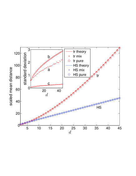
Figure 1: (Color online). Theoretical and numerical simulation results on the scaled mean trace distance $\sqrt{N}\mathcal{E}_{\mathrm{tr}}(\rho)$ and the scaled mean HS distance $\sqrt{N}\mathcal{E}_{\mathrm{HS}}(\rho)$ in state tomography with SIC POMs for $d$ from 2 to 45. The SIC POMs are generated by the Heisenberg-Weyl group from the fiducial states of Ref. RenBSC04b . The theoretical values are computed according to Eqs. (29) and (30), respectively, with $\rho=1/d$. $N=1000+20d^{2}$ is chosen in the numerical simulation. The values for the completely mixed state is the average over 1000 repeated experiments, and that for pure states is the average over 1000 randomly-generated pure states each averaged over 100 repeated experiments. The inset shows three kinds of standard deviations of the scaled mean trace distances for the numerical simulation. (a): the standard deviation over repeated experiments for the completely mixed state (the jumps in the curve are due to the finite number of experiments); (b): the average of the standard deviation over repeated experiments for each pure state; (c): the standard deviation over the randomly-generated pure states including a partial contribution of the fluctuation over the repeated experiments for each state due to the finite number of experiments.

Figure 1 shows the results of theoretical calculation and numerical simulation on state tomography with SIC POMs. The mean trace distance and the mean HS distance from numerical simulation agree perfectly with the theoretical formulae in Eqs. (29) and (30), in fact, much better than we have expected. The figure also clearly illustrates the different scaling behaviors of the two error measures with the dimension of the Hilbert space. From the inset of the figure, we see that the fluctuation in the mean trace distance over different pure states is much smaller than the fluctuation over repeated experiments on the same state. Actually, the former is so small that it is difficult to separate out the partial contribution of the latter with a limited number of repeated experiments. In other words, the reconstruction error is not sensitive to the identity of the true state.

We emphasize that the results on the tomographic efficiency of SIC POMs are representative of typical rank-one tight IC POMs. Since the order-3 frame potential $\Phi_{3}=(d^{2}+3d)/(d+1)^{2}$ for a SIC POM is much larger than the value $6d/(d+1)(d+2)$ required for a 3-design, a SIC POM is a very poor approximation of a 3-design, for which Eqs. (29) and (30) are best justified. Alternatively we can see this from the value of $\mathrm{Tr}\bigl{(}\mathcal{C}(\rho)^{2}\bigr{)}$ for a SIC POM, which can be computed according to Eqs. (4),

$$N^{2}\mathrm{Tr}\bigl{(}\mathcal{C}(\rho)^{2}\bigr{)} = \left(d^{2}+d+2\right)\bigl{[}1+\mathrm{tr}(\rho^{2})\bigr{]}-1$$ (32)

$${}+\bigl{[}\mathrm{tr}(\rho^{2})\bigr{]}^{2}-2(d^{2}+d)^{2}\sum_{j=1}^{d^{2}}p_{j}^{3}.\quad$$

When $d\gg 1$, the term $|\rho\rangle\!\rangle\langle\!\langle\rho|$ in the expression of $\mathcal{C}(\rho)$ can be neglected and we have

$$N^{2}\mathrm{Tr}\bigl{(}\mathcal{C}(\rho)^{2}\bigr{)} \approx (d^{2}+d)\bigl{[}1+\mathrm{tr}(\rho^{2})\bigr{]}.$$ (33)

Comparison with Eqs. (28) and (31) shows that the value $N^{2}\overline{\mathrm{Tr}\bigl{(}\mathcal{C}(\rho)^{2}\bigr{)}}$ for a SIC POM is roughly in the middle of the lower bound and the upper bound for tight IC measurements.

In the rest of this section, we briefly examine tight IC measurements that are not rank-one and which may arise in practice. In realistic experiments on quantum state tomography with a SIC POM, there always exists noise associated with detector inefficiency, dark counts, and other imperfections. It is important to understand how the noise affects tomographic efficiency. We investigate these effects with a simple white-noise model, in which the outcomes of the SIC POM are modified as follows,

$$\Pi_{j}(\alpha)=\frac{\alpha\frac{1}{d}+|\psi_{j}\rangle\langle\psi_{j}|}{d\alpha+d},$$ (34)

where the parameter $\alpha$ ($\alpha\geq 0$) characterizes the strength of the noise. This model is quite natural when there is no prior knowledge about the noise. Measurements of this form have also been considered in the context of entanglement detection with witness operators ZhuTE10a .

It is straightforward to verify that the measurement introduced above is still tight IC. The MSE can be calculated according to the procedure presented in Sec. II.1, with the result

$$\mathcal{E}_{\mathrm{M}}(\rho) = \frac{1}{N}\Bigl{\{}\frac{1}{d}\left[1+(d+1)^{2}(d-1)(\alpha+1)^{2}\right]-\mathrm{tr}(\rho^{2})\Bigr{\}}.$$

Compared with Eq. (19), the MSE is roughly $(\alpha+1)^{2}$ times as large as in the ideal case. The mean trace distance and the mean HS distance can still be computed according to Eqs. (25) and (26), respectively, with the result

$$\mathcal{E}_{\mathrm{tr}}(\rho) \approx \frac{4}{3\pi\sqrt{N}}(\alpha+1)d^{3/2},$$

$$\mathcal{E}_{\mathrm{HS}}(\rho) \approx \frac{1}{\sqrt{N}}(\alpha+1)d,$$ (36)

which are roughly $\alpha+1$ times the values for the ideal case. Hence, due to the noise, we need roughly $(\alpha+1)^{2}$ times as many copies of the true states to reach the same accuracy as in the ideal case. A similar analysis also applies to tight IC measurements derived from other 2-designs, such as complete sets of MUB.

III.4 Qubit SIC POM

In this section we provide further insights on the tomographic efficiency of the qubit SIC POM by deriving an exact formula for the mean trace distance and discussing the dependence of the reconstruction error on the Bloch vector of the true state (see Refs. RehEK04 ; LinLK08 ; BurLDG08 for earlier accounts). We also confirm that the result based on random matrix theory is already quite accurate for $d=2$, although it is best justified when $d$ is large. As a simple application, we make contact with the experimental result given by Ling et al. LinLK08 .

For the qubit SIC POM, the four outcomes $\Pi_{k}$ for $k=1,2,3,4$ are in one-to-one correspondence with the four unit vectors $\boldsymbol{a}_{k}$ pointing to the four vertices of a regular tetrahedron inscribed on the Bloch sphere; that is, $\Pi_{k}=\frac{1}{4}(1+\boldsymbol{a}_{k}\cdot\boldsymbol{\tau})$, where $\boldsymbol{\tau}=(\tau_{1},\tau_{2},\tau_{3})$ are the Pauli matrices ($\sigma_{j}$ are reserved to denote the standard deviations in this article). The reconstruction operators are given by $\Theta_{k}=\frac{1}{2}(1+3\boldsymbol{a}_{k}\cdot\boldsymbol{\tau})$ according to Eq. (18). Let $\boldsymbol{s}$ denote the Bloch vector of the true state $\rho$. To reconstruct the true state $\rho$ is equivalent to reconstruct the Bloch vector $\boldsymbol{s}$ RehEK04 ,

$$\rho = \sum_{k=1}^{4}p_{k}\Theta_{k}=\frac{1}{2}\biggl{(}1+3\sum_{k=1}^{4}p_{k}\boldsymbol{a}_{k}\cdot\boldsymbol{\tau}\biggr{)},$$

$$\boldsymbol{s} = 3\sum_{k=1}^{4}p_{k}\boldsymbol{a}_{k}.$$ (37)

Meanwhile, both the HS norm $|\!|\Delta\rho|\!|_{\mathrm{HS}}$ and the trace norm $|\!|\Delta\rho|\!|_{\mathrm{tr}}$ are proportional to the Euclidean length of $\Delta\boldsymbol{s}=\hat{\boldsymbol{s}}-\boldsymbol{s}$, where $\hat{\boldsymbol{s}}$ is an estimator of $\boldsymbol{s}$; that is, $|\!|\Delta\rho|\!|^{2}_{\mathrm{HS}}=(\Delta\boldsymbol{s})^{2}/2$, $|\!|\Delta\rho|\!|_{\mathrm{tr}}=|\Delta\boldsymbol{s}|/2$.

The MSE matrix of the estimator $\hat{\rho}$ can be calculated according to Eq.(4), with the result

$$\mathcal{C}(\rho) = \frac{3}{4}\biggl{(}\sum_{j=1}^{3}|\tau_{j}\rangle\!\rangle\langle\!\langle\tau_{j}|\biggr{)}-\frac{1}{4}|\boldsymbol{s}\cdot\boldsymbol{\tau}\rangle\!\rangle\langle\!\langle\boldsymbol{s}\cdot\boldsymbol{\tau}|$$

$${}+\frac{9}{16}\sum_{k=1}^{4}|\boldsymbol{a}_{k}\cdot\boldsymbol{\tau}\rangle\!\rangle\boldsymbol{a}_{k}\cdot\boldsymbol{s}\langle\!\langle\boldsymbol{a}_{k}\cdot\boldsymbol{\tau}|.$$

To get a concrete geometric picture, it is now better to work with the MSE matrix of the estimator $\hat{s}$ of the Bloch vector,

$$\mathcal{C}(\boldsymbol{s})=\frac{1}{N}\Bigl{[}3\boldsymbol{I}_{3}-\boldsymbol{s}\boldsymbol{s}+\frac{9}{4}\sum_{k}\left(\boldsymbol{a}_{k}\cdot\boldsymbol{s}\right)\boldsymbol{a}_{k}\boldsymbol{a}_{k}\Bigr{]},$$ (38)

where $\boldsymbol{I}_{3}$ is the $3\times 3$ identity dyadic. The mean squared error of the estimator $\hat{\boldsymbol{s}}$ is given by

$$\mathrm{E}(|\Delta\boldsymbol{s}|^{2}) = 2\mathcal{E}_{\mathrm{M}}(\rho)=\frac{1}{N}(9-s^{2}).$$ (39)

Suppose $\sigma_{1}^{2},\sigma_{2}^{2},\sigma_{3}^{2}$ are the three eigenvalues of the MSE matrix $\mathcal{C}(\boldsymbol{s})$, that is the three variances along the three principal axes of the uncertainty ellipsoid. Then the mean error is determined by the following integral,

$$\mathrm{E}(|\Delta\boldsymbol{s}|)=\int\mathrm{d}x\mathrm{d}y\mathrm{d}z\frac{\sqrt{x^{2}+y^{2}+z^{2}}}{(2\pi)^{3/2}\sigma_{1}\sigma_{2}\sigma_{3}}$$

$$\hphantom{\mathrm{E}(|\Delta\boldsymbol{s}|)=}\times\exp{\left[-\left(\frac{x^{2}}{2\sigma_{1}^{2}}+\frac{y^{2}}{2\sigma_{2}^{2}}+\frac{z^{2}}{2\sigma_{3}^{2}}\right)\right]}$$

$$=\sqrt{\frac{2}{\pi}}\int_{0}^{1}\mathrm{d}t\frac{\sigma_{1}^{2}\sigma_{3}^{2}+\sigma_{2}^{2}\sigma_{3}^{2},+(2\sigma_{1}^{2}\sigma_{2}^{2}-\sigma_{1}^{2}\sigma_{3}^{2}-\sigma_{2}^{2}\sigma_{3}^{2})t^{2}}{g^{3/2}},$$

where

$$g=\sigma_{3}^{2}(1-t^{2})^{2}+\frac{\sigma_{1}^{2}\sigma_{2}^{2}}{\sigma_{3}^{2}}t^{4}+(\sigma_{1}^{2}+\sigma_{2}^{2})t^{2}(1-t^{2}).$$

If at least two of the variances are equal, say $\sigma_{2}=\sigma_{1}$, then the integral can be evaluated explicitly,

$$\mathrm{E}(|\Delta\boldsymbol{s}|)=$$

$$\left\{\begin{array}[]{cl}{\displaystyle\sqrt{\frac{2}{\pi}}\sigma_{3}}&\mbox{if}\;\sigma_{1}=0,\\[4.30554pt] {\displaystyle\sqrt{\frac{\pi}{2}}\sigma_{1}}&\mbox{if}\;\sigma_{3}=0,\\[4.30554pt] {\displaystyle 2\sqrt{\frac{2}{\pi}}\sigma_{1}}&\mbox{if}\;\sigma_{3}=\sigma_{1},\\[4.30554pt] {\displaystyle\sqrt{\frac{2}{\pi}}\biggl{(}\frac{\sigma_{1}^{2}\arctan\sqrt{\frac{\sigma_{1}^{2}-\sigma_{3}^{2}}{\sigma_{3}^{2}}}}{\sqrt{\sigma_{1}^{2}-\sigma_{3}^{2}}}+\sigma_{3}\biggr{)}}&\mbox{if}\;\sigma_{1}>\sigma_{3},\\[8.61108pt] {\displaystyle\sqrt{\frac{2}{\pi}}\biggl{(}\frac{\sigma_{1}^{2}\mathrm{arctanh}\sqrt{\frac{\sigma_{3}^{2}-\sigma_{1}^{2}}{\sigma_{3}^{2}}}}{\sqrt{\sigma_{3}^{2}-\sigma_{1}^{2}}}+\sigma_{3}\biggr{)}}&\mbox{if}\;\sigma_{1}<\sigma_{3}.\end{array}\right.$$ (45)

If the uncertainty ellipsoid is isotropic, that is, $\sigma_{1}=\sigma_{2}=\sigma_{3}$, then we have

$$\mathcal{E}_{\mathrm{tr}}(\rho) = \sqrt{\frac{2}{3\pi N}}\sqrt{9-s^{2}}.$$ (46)

For the completely mixed state, this equation is exact, by contrast, the expression $\mathcal{E}_{\mathrm{tr}}(\rho)\approx 4\sqrt{9-s^{2}}/(3\pi\sqrt{N})$ based on random matrix theory [see Eq. (25)] is about $8\%$ smaller. The disparity is much smaller than the relative deviation of $|\!|\Delta\rho|\!|_{\mathrm{tr}}$ over repeated experiments, which is about $42\%$. For other true states, the disparity is even smaller. Hence, the result based on random matrix theory is already quite accurate even for $d=2$.

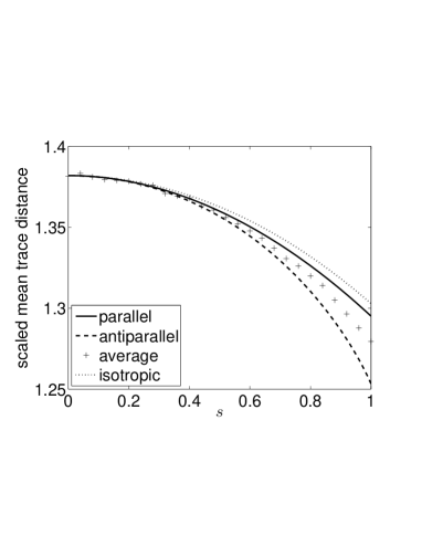
Figure 2: The scaled mean trace distances for states with Bloch vectors that are either parallel or antiparallel to the legs of the qubit SIC POM (theory), and the scaled mean trace distance averaged over randomly-generated states with a fixed purity (numerical simulation). $N=1000$ is chosen in the numerical simulation, and the scaled trace distance for each given purity is averaged over 1000 randomly-generated states each averaged over 400 repeated experiments. The dotted curve shows the scaled mean trace distance determined by Eq. (46), which assumes that the uncertainty ellipsoid is isotropic.

Those states whose Bloch vectors are either parallel or antiparallel to the legs of the SIC POM have attracted more attention both theoretically RehEK04 and experimentally LinLK08 , since they represent two extreme cases. We shall compute the mean trace distances for those states and discuss the dependence of the reconstruction error on the Bloch vector of the true state.

If $\boldsymbol{a}_{1}$ is chosen as the $z$ axis, without loss of generality, the Bloch vectors of those extreme states can be parameterized as $\boldsymbol{s}=z\boldsymbol{a}_{1}$ with $-1\leq z\leq 1$. According to Eq. (38), the MSE matrix of $\hat{\boldsymbol{s}}$ now reads

$$\mathcal{C}(s)=\frac{(3-z)\boldsymbol{I}_{3}+(3z-z^{2})\boldsymbol{a}_{1}\boldsymbol{a}_{1}}{N},$$ (47)

whose eigenvalues are given by

$$\sigma_{1}^{2}=\sigma_{2}^{2}=\frac{3-z}{N},\quad\sigma_{3}^{2}=\frac{(3-z)(1+z)}{N}.$$ (48)

Note that the uncertainty ellipsoid is rotationally symmetric. As $z$ decreases from $1$ to $-1$, the uncertainty ellipsoid evolves from prolate to oblate and finally to a singular ellipsoid when $z=-1$. The mean trace distance of those extreme states can be calculated according to Eq. (III.4). Figure 2 shows the scaled mean trace distances for those states together with the numerical average over randomly-generated states. The mean trace distance is slightly smaller for states with Bloch vectors that are antiparallel to the legs of the SIC POM than those that are parallel. For a fixed purity of the true states, the average of the mean trace distance over randomly-generated states sits roughly in the middle of the two extreme cases. In all three cases, there is a slight decrease in the mean trace distance as the purity of the true state increases, which can roughly be attributed to two reasons: the decrease in the MSEs [cf. Eq. (39)] and the increase in the degrees of anisotropy of the uncertainty ellipsoids.

Ling et al. LinLK08 have studied the tomographic efficiency of the qubit SIC POM experimentally and determined the scaled mean trace distances for the three states with $z=0,-1,1$, respectively, with the result $1.417,1.288,1.323$. By contrast, our theoretical calculation has yielded the result $1.382,1.259,1.295$. The experimental and the theoretical values reflect the same dependence of the reconstruction error on the Bloch vector of the true state. The former are slightly larger than the latter, but the difference is very small, in other words, the agreement between experimental data and theoretical calculation is pretty good. Note that the relative fluctuation of the reconstruction error over repeated experiments is larger than $40\%$ and the experimental values are the average of only 40 runs. In addition, any imperfection inevitable in real experiments may also affect the accuracy of the estimator.

IV Joint SIC POMs and Product SIC POMs

In the bipartite or multipartite settings, it is technologically much more challenging and sometimes even impossible to perform full joint measurements such as SIC POMs on the whole system. It is thus of paramount practical interests to determine the optimal product measurements and the efficiency gap between the product measurements and the joint measurements. We show that under linear state tomography, product SIC POMs are optimal among all product measurements in the same sense as joint SIC POMs are optimal among all joint measurements. Furthermore, in the bipartite setting, there is only a marginal efficiency advantage of the joint SIC POMs over the product SIC POMs and it is thus not worth the trouble to perform the joint measurements. However, in the multipartite settings, the efficiency advantage of the joint SIC POMs over the product SIC POMs increases exponentially with the number of parties.

IV.1 Bipartite SIC POMs and product SIC POMs

Consider a product measurement on a bipartite system whose parts $A,B$ have subsystem dimensions $d_{1},d_{2}$ respectively, and the total dimension is $d=d_{1}d_{2}$. To show the optimality of the product SIC POM, we shall use the same strategy described in Sec. II.3. More generally, we show that if the product measurement minimizes the MSE averaged over unitarily equivalent states, then the measurement on each subsystem is rank-one tight IC, and vice versa. As an immediate consequence, the product SIC POM is optimal and furthermore any minimal optimal product measurement must be a product SIC POM, recall that SIC POMs are the only minimal tight IC measurements Sco06 .

Since the average of $\rho$ is the completely mixed state, it suffices to demonstrate our claim when $\rho=1/d$ according to Eq. (4). Suppose $\Pi_{j_{1}}$ are the outcomes of the measurement on the first subsystem and $\Pi_{j_{2}}$ are those for the second subsystem, then each outcome in the product measurement has a tensor product form $\Pi_{j_{1}j_{2}}=\Pi_{j_{1}}\otimes\Pi_{j_{2}}$. The same is true for the frame superoperator $\mathcal{F}=\mathcal{F}_{1}\otimes\mathcal{F}_{2}$ and the reconstruction operators $\Theta_{j_{1}j_{2}}=\Theta_{j_{1}}\otimes\Theta_{j_{2}}$. According to Eq. (II.3), we have

$$\mathcal{C}\Bigl{(}\frac{1}{d}\Bigr{)} = \frac{1}{N}\Bigl{(}\frac{\mathcal{F}_{1}^{-1}\otimes\mathcal{F}_{2}^{-1}}{d}-\frac{\mathcal{I}}{d^{2}}\Bigr{)},$$

$$\mathcal{E}_{\mathrm{M}}\Bigl{(}\frac{1}{d}\Bigr{)} = \frac{1}{dN}\bigl{[}\mathrm{Tr}\bigl{(}\mathcal{F}_{1}^{-1}\bigr{)}\mathrm{Tr}\bigl{(}\mathcal{F}_{2}^{-1}\bigr{)}-1\bigr{]}.$$ (49)

The MSE is minimized if and only if both $\mathrm{Tr}\bigl{(}\mathcal{F}_{1}^{-1}\bigr{)}$ and $\mathrm{Tr}\bigl{(}\mathcal{F}_{2}^{-1}\bigr{)}$ are minimized, that is, when the measurement on each subsystem is rank-one tight IC (cf. Sec. II.3).

Next, let us focus on the tomographic efficiency of the optimal product measurements. If the product measurement is composed of two rank-one tight IC measurements, as in the case of the product SIC POM, then each factor in the reconstruction operator $\Theta_{j_{1}j_{2}}=\Theta_{j_{1}}\otimes\Theta_{j_{2}}$ is given by Eq. (18). The MSE can be computed according to Eq. (5),

$$\mathcal{E}^{\mathrm{prod}}_{\mathrm{M}}(\rho)=\frac{1}{N}\bigl{[}(d_{1}^{2}+d_{1}-1)(d_{2}^{2}+d_{2}-1)-\mathrm{tr}(\rho^{2})\bigr{]}.\quad$$ (50)

Surprisingly, the MSE is almost independent of the true state, as in the case of SIC POMs. In addition, it is approximately equal to the product of the MSEs for two subsystems, respectively. The variance $v^{\mathrm{prod}}(\rho)$ of the squared error may depend on the specific choice of product measurements according to Eq. (7). For the product SIC POM, it is approximately given by

$$v^{\mathrm{prod}}(\rho)\approx\frac{2}{N^{2}}\Big{\{}(d_{1}^{2}+d_{1}-2)(d_{2}^{2}+d_{2}-2)$$

$$\quad{}\times\bigl{[}1+\mathrm{tr}(\rho^{2})+\mathrm{tr}(\rho_{1}^{2})+\mathrm{tr}(\rho_{2}^{2})\bigr{]}+(d_{1}^{2}+d_{1}-2)$$

$$\quad{}\times\bigl{[}1+\mathrm{tr}(\rho_{1}^{2})\bigr{]}+(d_{2}^{2}+d_{2}-2)\bigl{[}1+\mathrm{tr}(\rho_{2}^{2})\bigr{]}\Big{\}}.\quad$$ (51)

Note that the variance does not only depend on the purity of the global state, but also on the purities of the reduced states, which means that it generally depends on the entanglement of the global state. For example, if the true state is pure, the variance is approximately maximized for product states and minimized for maximally entangled states.

Compared with the result of the joint SIC POM given in Eq. (19), the MSE achieved by the product SIC POM is slightly larger, but the difference is generally very small, especially when both $d_{1}$ and $d_{2}$ are large. By contrast, the fluctuation over repeated experiments is stronger by a bigger margin in the product SIC POM. Figure 3 shows the ratio of the MSEs when the true state is the completely mixed state, note that the ratio for other true states is almost the same. The maximal ratio $1.36$ is obtained when $d_{1}=d_{2}=3$. If $d_{1},d_{2}\geq 3$, the ratio decreases monotonically with $d_{1}$ and $d_{2}$; if $d_{2}=2$ and $d_{1}\geq 3$, the ratio decreases monotonically with $d_{1}$. For sufficiently large $d_{1},d_{2}$, the ratio is about $1+1/d_{1}+1/d_{2}$. In conclusion, there is only a marginal efficiency advantage of the joint SIC POM over the product SIC POM. The product SIC POM is thus more appealing for practical applications since it is much easier to be implemented.

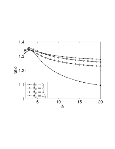
Figure 3: The ratio of the MSEs in state tomography with the product SIC POM and the joint SIC POM when the true state is the completely mixed state, note that the ratios for other true states are almost the same. The ratio is maximized when $d_{1}=d_{2}=3$. The ratio of the mean trace distances is approximately equal to the square root of the ratio of the MSEs.

Although the product SIC POM is not even a tight IC measurement, comparison of Eqs. (50) and (IV.1) shows that the relative deviation of the squared error is quite small, especially when $d_{1},d_{2}$ are large. Hence, Eq. (26) is still a good approximation for computing the mean HS distance. The mean trace distance can be calculated approximately according to Eq. (25), with the result

$$\mathcal{E}_{\mathrm{tr}}(\rho)\approx\frac{4\sqrt{d_{1}d_{2}}}{3\pi\sqrt{N}}\sqrt{(d_{1}^{2}+d_{1}-1)(d_{2}^{2}+d_{2}-1)-\mathrm{tr}(\rho^{2})}.$$

Generally speaking, the larger the values of $d_{1}$ and $d_{2}$ are, the more accurate is this formula. The ratio of the mean trace distance with the product SIC POM to that with the joint SIC POM is thus approximately equal to the square root of the ratio of the MSEs.

Table 1 shows the theoretical and numerical simulation results on the scaled mean trace distances for the two-qubit product SIC POM and joint SIC POM. There is quite a good agreement between theoretical calculation and numerical simulation although $d_{1}$ and $d_{2}$ are so small. The mean trace distances achieved by the product SIC POM are roughly $15\%$ larger than that achieved by the joint SIC POM. As a consequence, with the product SIC POM, we need about $32\%$ more copies of the true states to reach the same accuracy achieved by the joint SIC POM. Despite its slightly lower efficiency, the product SIC POM is more appealing than the joint SIC POM due to the relative ease in its implementation in real experiments. The same conclusion has also been reached in Ref. TeoZE10 , where the maximum-likelihood method was adopted for state reconstruction.

Table 1: Theoretical and numerical simulation results of the scaled mean trace distances for the two-qubit joint SIC POM (Joint) and product SIC POM (Prod). The theoretical values are computed according to Eqs. (29) and (IV.1), respectively. $N=1000$ is chosen for the numerical simulation. For the completely mixed state, the scaled trace distance is averaged over 1000 repeated experiments. For pure states, it is averaged over $1000$ randomly-generated states, each averaged over 1000 repeated experiments. The standard deviations of the scaled trace distances over the 1000 randomly-generated pure states (including a partial contribution of the fluctuation over the repeated experiments for each state due to the finite number of experiments) are 0.033 and 0.027 for the product SIC POM and the joint SIC POM, respectively, both of which are very small.

	Completely mixed state			Average over pure states
POM	Theory	Numerical	Error%	Theory	Numerical	Error%
Prod	4.223	4.255	$-0.8$	4.158	4.162	$-0.1$
Joint	3.676	3.716	$-1.1$	3.601	3.575	$+0.7$
Ratio	1.149	1.145	—	1.155	1.164	—

IV.2 Multipartite SIC POMs and product SIC POMs

Suppose $k$ parties want to reconstruct a quantum state shared among them with a product measurement, and $d_{j}$ for $j=1,2,\cdots,k$ is the dimension of the Hilbert space of the $j$th party. According to the same analysis as in the bipartite setting, under linear state tomography, the product SIC POM is optimal among all product measurements. The MSE achieved by the product SIC POM can also be calculated in the same manner, with the result

$$\mathcal{E}_{\mathrm{M}}^{\mathrm{prod}}(\rho)=\frac{1}{N}\biggl{[}\prod_{j=1}^{k}(d_{j}^{2}+d_{j}-1)-\mathrm{tr}(\rho^{2})\biggr{]},$$ (53)

which is almost independent of the true state. When the true state is the completely mixed state, the variance of the squared error is given by

$$v^{\mathrm{prod}}(\rho)=\frac{2}{N^{2}}\biggl{[}\prod_{j=1}^{k}\frac{(d_{j}^{3}+2d_{j}^{2}-2)}{d_{j}}-\prod_{j=1}^{k}\frac{1}{d_{j}^{2}}\biggr{]}.$$ (54)

For a generic true state, the variance depends on the purity of the global state as well as the purities of various reduced states, and can be much larger than the value given above.

If the dimension of the Hilbert space of each party is equal to $d_{1}$, then the ratio of the MSE for the product SIC POM to that for the joint SIC POM grows exponentially with the number of parties $k$,

$$\frac{\mathcal{E}_{\mathrm{M}}^{\mathrm{prod}}(\rho)}{\mathcal{E}_{\mathrm{M}}^{\mathrm{joint}}(\rho)}\approx\left(1+\frac{1}{d}-\frac{1}{d^{2}}\right)^{-1}\left(1+\frac{1}{d_{1}}-\frac{1}{d_{1}^{2}}\right)^{k}.$$ (55)

The ratio of the variances grows with an even higher rate, whose specific value may heavily depend on the true state. In other words, the efficiency advantage of the joint SIC POM over the product SIC POM grows exponentially with the number of parties.

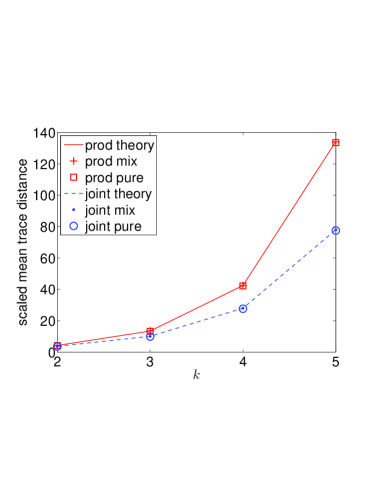
Figure 4: (Color online). Theoretical and numerical simulation results of the scaled mean trace distances for the joint SIC POMs and the product SIC POMs on multiqubit systems, where $k$ is the number of qubits. The theoretical values are computed according to Eqs. (29) and (56), respectively, with $\rho=1/d$. $N=1000+20d^{2}$ is chosen in the numerical simulation. For the completely mixed state, the scaled trace distance is averaged over 1000 repeated experiments. For pure states, it is averaged over $1000$ randomly-generated states, each averaged over 100 repeated experiments.

Although the fluctuation in the reconstruction error over repeated experiments is stronger in the product SIC POMs as compared with the joint SIC POMs, the relative fluctuation is still small. Hence, Eq. (26) is still a good approximation for computing the mean HS distance. When $k$ is not too large, the mean trace distance can be calculated approximately according to Eq. (25), with the result

$$\mathcal{E}_{\mathrm{tr}}(\rho) \approx \frac{4\sqrt{d}}{3\pi\sqrt{N}}\sqrt{\prod_{j=1}^{k}\left(d_{j}^{2}+d_{j}-1\right)-\mathrm{tr}(\rho^{2})}.$$ (56)

Since the ratio of the mean trace distance achieved by the product SIC POM to that achieved by the joint SIC POM is approximately equal to the square root of the ratio of the MSEs, it also increases exponentially with the number of parties; the same is true for the mean HS distance. Figure 4 shows theoretical and numerical simulation results of the scaled mean trace distances for the product SIC POMs and the joint SIC POMs on multiqubit systems (numerical fiducial kets of SIC POMs are available at Ref. RenBSC04b ). There is a pretty good agreement between theoretical prediction and numerical simulation for $k$ up to 5. This plot further confirms that the efficiency advantage of the joint SIC POM over the product SIC POM increases exponentially with the number of parties.

V Summary

We have introduced random matrix theory Meh04 for studying the tomographic efficiency of tight IC measurements, which include SIC POMs as a special example. In particular, we derived analytical formulae for the mean trace distance and the mean HS distance between the estimator and the true state and showed the different scaling behaviors of the two error measures with the dimension of the Hilbert space. The accuracy of these formulae were confirmed by extensive numerical simulations on state tomography with SIC POMs. In the special case of the qubit SIC POM, we derived an exact formula for the mean trace distance and discussed in detail the dependence of the reconstruction error on the Bloch vector of the unknown true state. As a byproduct, we also discovered a special class of tight IC measurements called isotropic measurements, which feature exceptionally symmetric outcome statistics and low fluctuation over repeated experiments.

In the bipartite and multipartite settings, we showed that the product SIC POMs are optimal among all product measurements in the same sense as the joint SIC POMs are optimal among all joint measurements. We further showed that for bipartite systems, there is only a marginal efficiency advantage of the joint SIC POMs over the product SIC POMs, which disappears in the large-dimension limit. Hence, it is not worth the trouble to perform the joint measurements at the current stage. However, for multipartite systems, the efficiency advantage of the joint SIC POMs over the product SIC POMs increases exponentially with the number of parties.

Our study provided a simple picture of the scaling behavior of the resource requirement in state tomography with the dimension of the Hilbert space, and of the efficiency gap between product measurements and joint measurements. The idea of applying random matrix theory to studying tomographic efficiencies may also find wider applications in other state estimation problems.

References

- (1) Quantum State Estimation, edited by M. G. A. Paris and J. Řeháček, Lecture Notes in Physics, Vol. 649 (Springer, Berlin, 2004).
- (2) A. I. Lvovsky and M. G. Raymer, Rev. Mod. Phys. 81, 299 (2009).
- (3) E. Prugovečki, Int. J. Theor. Phys. 16, 321 (1977).
- (4) P. Busch, Int. J. Theor. Phys. 30, 1217 (1991).
- (5) G. M. D’Ariano, P. Perinotti, and M. F. Sacchi, J. Opt. B: Quantum Semiclassical Opt. 6, S487 (2004).
- (6) A. J. Scott, J. Phys. A: Math. Gen. 39, 13507 (2006).
- (7) A. Roy and A. J. Scott, J. Math. Phys. 48, 072110 (2007).
- (8) G. Zauner, Int. J. Quant. Inf. 9, 445 (2011).
- (9) J. M. Renes, R. Blume-Kohout, A. J. Scott, and C. M. Caves, J. Math. Phys. 45, 2171 (2004).
- (10) D. M. Appleby, J. Math. Phys. 46, 052107 (2005).
- (11) A. J. Scott and M. Grassl, J. Math. Phys. 51, 042203 (2010).
- (12) J. Řeháček, B.-G. Englert, and D. Kaszlikowski, Phys. Rev. A 70, 052321 (2004).
- (13) The analytical solutions for and were reported by Markus Grassl in private communication (April and May 2011).
-
(14)
Available online at
http://info.phys.unm.edu/papers/
reports/sicpovm.html - (15) I. D. Ivanović, J. Phys. A: Math. Gen. 14, 3241 (1981).
- (16) W. K. Wootters and B. D. Fields, Ann. Phys. (N.Y.) 191, 363 (1989).
- (17) W. K. Wootters, Found. Phys. 36, 112 (2006).
- (18) D. M. Appleby, AIP Conf. Proc. 1101, 223 (2009).
- (19) T. Durt, B.-G. Englert, I. Bengtsson, and K. Życzkowski, Int. J. Quant. Inf. 8, 535 (2010).
- (20) P. W. H. Lemmens and J. J. Seidel, J. Algebra 24, 494 (1973).
- (21) D. M. Appleby, S. T. Flammia, and C. A. Fuchs, J. Math. Phys. 52, 022202 (2011).
- (22) C. A. Fuchs, e-print arXiv:1003.5209v1 [quant-ph].
- (23) M. A. Nielsen and I. L. Chuang, Quantum Computation and Quantum Information (Cambridge University Press, Cambridge, UK, 2000).
- (24) I. Bengtsson and K. Życzkowski, Geometry of Quantum States, An Introduction to Quantum entanglement (Cambridge University Press, Cambridge, UK, 2006).
- (25) R. Horodecki, P. Horodecki, M. Horodecki, and K. Horodecki, Rev. Mod. Phys. 81, 865 (2009).
- (26) C. A. Fuchs and J. van de Graaf, IEEE Trans. Inf. Theory 45, 1216 (1999).
- (27) A. Ling, A. Lamas-Linares, and C. Kurtsiefer, e-print arXiv:0807.0991v1 [quant-ph].
- (28) M. D. de Burgh, N. K. Langford, A. C. Doherty, and A. Gilchrist, Phys. Rev. A 78, 052122 (2008).
- (29) Y. C. Liang, D. Kaszlikowski, B.-G. Englert, L.-C. Kwek, and C. H. Oh, Phys. Rev. A 68, 022324 (2003).
- (30) B.-G. Englert, D. Kaszlikowski, J. Řeháček, H. K. Ng, W. K. Chua, and J. Anders, e-print arXiv:quant-ph/0412075.
- (31) T. Durt, C. Kurtsiefer, A. Lamas-Linares, and A. Ling, Phys. Rev. A 78, 042338 (2008).
- (32) Y. S. Teo, H. Zhu, and B.-G. Englert, Opt. Commun. 283, 724 (2010).
- (33) M. L. Mehta, Random Matrices (Elsevier, Amsterdam, third edition, 2004).
- (34) Z. Hradil, Phys. Rev. A 55, R1561 (1997).
- (35) G. M. D’Ariano, P. Lo Presti, and M. F. Sacchi, Phys. Lett. A 272, 32 (2000).
- (36) G. M. D’Ariano and P. Perinotti, Phys. Rev. Lett. 98, 020403 (2007).
- (37) P. Rungta, W. J. Munro, K. Nemoto, P. Deuar, G. J. Milburn, and C. M. Caves, Qudit entanglement, in Directions in Quantum Optics: A Collection of Papers Dedicated to the Memory of Dan Walls, edited by H. J. Carmichael, R. J. Glauber, and M. O. Scully, p. 149 (Springer, Berlin, 2000).
- (38) P. Rungta, V. Bužek, C. M. Caves, M. Hillery, and G. J. Milburn, Phys. Rev. A 64, 042315 (2001).
- (39) R. J. Duffin and A. C. Schaeffer, Trans. Am. Math. Soc. 72, 341 (1952).
- (40) P. G. Casazza, Taiw. J. Math. 4, 129 (2000).
- (41) P. D. Seymour and T. Zaslavsky, Adv. Math. 52, 213 (1984).
- (42) S. G. Hoggar, Eur. J. Combinator. 3, 233 (1982).
- (43) H. Zhu, Y. S. Teo, and B.-G. Englert, Phys. Rev. A 81, 052339 (2010).