Master equations for correlated quantum channels

Abstract

We derive the general form of a master equation describing the interaction of an arbitrary multipartite quantum system, consisting of a set of subsystems, with an environment, consisting of a large number of sub-envirobments. Each subsystem “collides” with the same sequence of sub-environments which, in between the collisions, evolve according to a map that mimics relaxations effects. No assumption is made on the specific nature of neither the system nor the environment. In the weak coupling regime, we show that the collisional model produces a correlated Markovian evolution for the joint density matrix of the multipartite system. The associated Linblad super-operator contains pairwise terms describing cross correlation between the different subsystems.

In the study of the open dynamics of a multipartite quantum system ${\cal S}$ the simplifying assumption that each subsystem interacts with its own local environment is frequently made. In quantum communication BENSHOR where ${\cal S}$ is identified with the set of information carriers employed in the signaling process, this is equivalent to saying that a given communication channel is memoryless i.e. that it acts independently on each separate carrier. In recent years, however, the study of correlated channels - sometimes called also channels with memory - has shown that interesting new features emerge when one makes the realistic assumption that the action of the noise tampering with the communication line is correlated over consecutive carriers (e.g. see MPV ; BM ; KW ; VJP ; PV ; LUPO ; DARRIGO and references therein). Such correlations have been phenomenologically described in terms of a Markov chain which gives the joint probability distribution of the local Kraus operators acting on the elements of ${\cal S}$ MPV . Alternatively they have been effectively represented in terms of local interactions of the carriers with a common multipartite environment which is originally prepared into a correlated (possibly entangled) initial state PV , or with a structured environment composed by local and global components BM ; KW ; VJP .

The aim of the present paper is to provide a continuous time description of correlated quantum channels in terms of a joint Master Equation (ME) LIND ; PET for ${\cal S}$. This will lead us to identify the structure of the Lindblad generators which are responsible for the arising of specific correlations among the carriers. We remind that determining if a given quantum transformation is compatible with a Lindblad structure is in general a computationally hard problem NONMARK . Also we notice that a Lindbladian structure for the global system ${\cal S}$ in general may introduce non-Markovian elements in the dynamics of the subsystems that compose it, which also are far from trivial to characterize, e.g. see Refs. BRVC . To bypass such difficulties in our analysis we will thus adopt a rather pragmatic approach, deriving the dynamical evolution of ${\cal S}$ from a collisional model SZS ; ZSB in which dissipative effects originate from a sequence of weak but frequent interactions with a collection of uncorrelated particles which mimic the system environment.

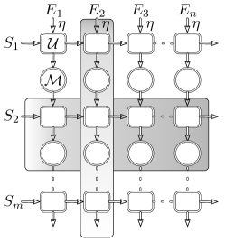
Figure 1: Schematic of the process. The horizontal lines describe an ordered set of carriers $S_{1},S_{2},\cdots$ which interact with an ordered set of (possibly infinite) identical local sub-environments $E_{1},E_{2},\cdots$ via local unitaries $\mathcal{U}_{S_{m}E_{n}}$. Between collisions each sub-environment evolves according to a map $\mathcal{M}$. The overall dynamics can be described as a ordered sequence of row or of column super-operators (visualized by the rectangular sets in the figure).

Consider hence a multipartite quantum system ${\cal S}$, consisting of $M$ - not necessarily identical - ordered subsystems $S_{1},S_{2},\cdots,S_{M}$. In what follows each subsystem is supposed to interact with a multipartite environment ${\cal E}$ consisting of a large number of sub-environments $E_{1},E_{2},\cdots$ via an ordered sequence of pairwise interactions (for a pictorial representation see Fig. 1). As in SZS ; ZSB the pairwise collision between the subsystem $S_{m}$ and the sub-envirinment $E_{n}$ is described by a local unitary $U_{S_{m}E_{n}}=\exp[-igH_{S_{m}E_{n}}\Delta t]$ characterized by a collision time $\Delta t$ and by the intensity parameter $g$, and generated by the Hamiltonian coupling $H_{S_{m}E_{n}}$ which (without loss of generality) we write as

$$H_{S_{m}E_{n}}:=\sum_{\ell}\;A^{(\ell)}_{S_{m}}\otimes B^{(\ell)}_{E_{n}}\;,$$ (1)

with $A^{(\ell)}_{S},B^{(\ell)}_{E}\neq 0$ Hermitian. Accordingly the $m$-th carrier interacts with the first $n$ elements of the environment ${\cal E}$ through the joint unitary

$$U_{S_{m}{\cal E}}^{(n)}:=U_{S_{m},E_{n}}\;U_{S_{m},E_{n-1}}\;\cdots\;U_{S_{m},E_{2}}\;U_{S_{m},E_{1}}\;,$$ (2)

(the presence of a local free Hamiltonian evolution operating between the collisions can be included in the model by passing into the interaction picture representation and replacing $A^{(\ell)}_{S_{m}}$ with the corresponding evolved operators). Finally to account for the internal dynamics of the environment, we assume that between two consecutive collisions each sub-environment evolves according to a completely, positive, trace preserving (CPT) map $\mathcal{M}$.

Consider then the case where the $M$ subsystems of ${\cal S}$ are initially in a (possibly correlated) state $\rho(0)$ while the sub-environments of ${\cal E}$ are all prepared into the same input state $\eta$ (which, as in Ref. SZS , represents some equilibrium state of the particles of the reservoir). For the sake of simplicity in the following we will work under the hypothesis that

$$~{}\langle B_{E}^{(\ell)}{\cal M}^{m}(\eta)\rangle_{E}=0\qquad\forall\ell,m\;,$$ (3)

where we use the symbol $\langle\cdots\rangle_{X}$ to represent the trace over the system ${X}$, and ${\cal M}^{m}$ to represent the channel obtained by applying $m$ times the map ${\cal M}$. The assumption (3) allows us to rigorously define the continuous limit of the model. It is worth noticing however that it does not imply any loss of generality as it can always be enforced by moving into an interaction representation with respect to a rescaled local Hamiltonian for the system ${\cal S}$.

After the interactions with the first $n$ element of ${\cal E}$ the global state $R(n)$ of the system and of the environment is obtained from the initial state $\rho(0)\otimes\eta^{\otimes n}$ as $R(n)={\cal W}^{(n,M)}(\rho(0)\otimes\eta^{\otimes n})$, where ${\cal W}^{(n,M)}$ is the super-operator which describes the collisions and the free evolutions of ${\cal E}$. As schematically shown in Fig. 1, it can be expressed as a composition of row super-operators stack in series one on top of the other

$${\cal W}^{(n,M)}={\cal R}_{S_{M},{\cal E}}\circ{\cal R}_{S_{M-1},{\cal E}}\circ\cdots\circ{\cal R}_{S_{2},{\cal E}}\circ{\cal R}_{S_{1},{\cal E}}\;,$$ (4)

where ${\cal R}_{S_{m},{\cal E}}:={\cal M}^{\otimes n}\;\circ\;{\cal U}_{S_{m},{\cal E}}^{(n)}$. Here given, a unitary transformation $U$, we define ${\cal U}(\cdots)=U(\cdots)U^{\dagger}$. Also we use the symbol “$\circ$” to represent the composition of super-operators and ${\cal M}^{\otimes n}$ to represent ${\cal M}_{E_{1}}\circ\cdots\circ{\cal M}_{E_{n}}$, ${\cal M}_{E_{j}}$ being the map ${\cal M}$ operating on the $j$-th element ${E}_{j}$ of ${\cal E}$. The transformation ${\cal R}_{S_{m},{\cal E}}$ describes the evolution of $S_{m}$ in its interaction with ${\cal E}$ plus the subsequent free evolution of the latter induced by the maps $\cal M$. Alternatively, exploiting the fact that for $m^{\prime}\neq m$, $n^{\prime}\neq n$ the operators $U_{S_{m},E_{n}}$ and $U_{S_{m^{\prime}},E_{n^{\prime}}}$ commute, ${\cal W}^{(n,M)}$ can also be expressed in terms of column super-operators concatenated in series as follows:

$${\cal W}^{(n,M)}={\cal C}_{{\cal S},E_{n}}\circ{\cal C}_{{\cal S},E_{n-1}}\circ\cdots\circ{\cal C}_{{\cal S},E_{2}}\circ{\cal C}_{{\cal S},E_{1}}\;,$$ (5)

where for all $j=1,\cdots,n$,

$${\cal C}_{{\cal S},E_{j}} := {\cal M}_{E_{j}}\circ{\cal U}_{S_{M},E_{j}}\circ\cdots\circ{\cal M}_{E_{j}}\circ{\cal U}_{S_{1},E_{j}}\;.$$ (6)

Thanks to Eq. (5) we can now write the following recursive expression for $R(n)$:

$$R(n+1) = {\cal C}_{{\cal S},E_{n+1}}(R(n)\otimes\eta)\;.$$ (7)

I The Master Equation

For a particular class of interaction unitaries, the Authors of ZSB have shown that the collision model leads to a dynamics which can be described by a Lindblad super-operator via direct integration of the equation of motion. Here we introduce an alternative approach which allows one to derive a ME for the reduced dynamics of the many-body system $\mathcal{S}$ in our generalized multipartite collision model. The details of the derivation can be found in the Appendix. We simply assume a weak coupling regime where we take a proper expansion with respect to the parameters $g$ and $\Delta t$ which quantifies the intensity and the duration of the single events. In particular we work in the regime in which $g\Delta t$ is a small quantity and expand the dynamical equation (7) up to ${\cal O}\big{(}(g\Delta t)^{2}\big{)}$, i.e.

$$R(n+1) = \big{[}{\cal I}_{{\cal S},E_{n+1}}+{\cal C}^{\prime}_{{\cal S},E_{n+1}}g\Delta t$$

$$+ {\cal C}^{\prime\prime}_{{\cal S},E_{n+1}}(g\Delta t)^{2}\big{]}(R(n)\otimes\eta)+{\cal O}\big{(}(g\Delta t)^{3}\big{)}\;,$$

where ${\cal I}_{{\cal S},E_{n+1}}$ is the identity superoperator while ${\cal C}^{\prime}_{{\cal S},E_{n+1}}$ and ${\cal C}^{\prime\prime}_{{\cal S},E_{n+1}}$ are the first and second expansion terms in $g\Delta t$ of the superoperator ${\cal C}_{{\cal S},E_{n+1}}$, respectively. Tracing over the degree of freedom of the environment the resulting equation defines the incremental evolution of the density matrix $\rho(n):=\langle R(n)\rangle_{\cal E}$ of ${\cal S}$ when passing from the $n$-th to the $(n+1)$-th collision. The continuos limit is finally taken by sending $\Delta t$ to zero while $g$ and $n$ explode in such a way that $n\Delta t$ and $g^{2}\Delta t$ remains finite, i.e.

$$\lim_{\Delta t\rightarrow 0^{+}}n\;\Delta t=t<\infty\;,\quad\lim_{\Delta t\rightarrow 0^{+}}g^{2}\Delta t=\gamma<\infty\;.$$ (9)

Notice that while the first condition is necessary to properly define the axis of time, the second is needed to guarantee that ${\cal S}$ fills the interactions with ${\cal E}$. Indeed one easily verifies that the linear terms in $g$ do not enter in the dynamical evolution of $\cal S$ since $\langle{\cal C}^{(1)}_{{\cal S},E_{n+1}}(R(n)\otimes\eta)\rangle_{\cal E}=0$ due to the assumption (3).

Defining hence $\rho(t)=\lim_{\Delta t\rightarrow 0^{+}}\;\rho(n)$ the reduced density matrix of ${\cal S}$ at time $t$, and $\dot{\rho}(t):=\lim_{\Delta t\rightarrow 0^{+}}\;\tfrac{\rho(n+1)-\rho(n)}{\Delta t}$ its time derivative, from Eq. (I) we get the following ME:

$${\dot{\rho}}(t)=\sum_{m=1}^{M}{\cal L}_{m}(\rho(t))+\sum_{m^{\prime}>m}{\cal D}^{(\rightarrow)}_{m,m^{\prime}}(\rho(t))\;.$$ (10)

This is mathematically equivalent to the standard derivation of a Markovian ME for a system inetracting with a large environment, in which one assumes that the overall system-environment density operator at any given time $t$ of the evolution factorizes as in $\rho(t)\otimes\eta$ where $\eta$ is the environment density operator. The two scenarios are however different. In the standard case the reason for which the environment state is unchanged is because it is big. In our scenario, consistently with the collision model, the environment state is constant because, as we said, each subsystem collides briefly with a sequence of sub-environments all initially in the same state. Of course one expects a strongly non markovian behavior if a given subsystem interacts repeatedly with the same sub-environment BP .

The ME (10) contains both local Lindblad terms (i.e. Lindblad terms which act locally on the $m$-th carrier) and two-body non local terms which couple the $M$ carrier with the $m^{\prime}>m$. More precisely the $m$-th local term is the super-operator

$${\cal L}_{m}(\cdots) = \frac{1}{2}\sum_{\ell,\ell^{\prime}}{\gamma_{m}^{(\ell,\ell^{\prime})}}\big{[}2A_{S_{m}}^{(\ell^{\prime})}(\cdots)A_{S_{m}}^{(\ell)}$$ (11)

$$-A^{(\ell)}_{S_{m}}A^{(\ell^{\prime})}_{S_{m}}(\cdots)-(\cdots)A^{(\ell)}_{S_{m}}A^{(\ell^{\prime})}_{S_{m}}\big{]}\;,$$

where the non negative matrix $\gamma^{(\ell,\ell^{\prime})}_{m}$ is given by

$$\gamma^{(\ell,\ell^{\prime})}_{m}:=\gamma\;\langle B_{E}^{(\ell)}B_{E}^{(\ell^{\prime})}\;{\cal M}^{m-1}(\eta)\rangle_{E}\;,$$ (12)

with $\gamma$ as in Eq. (9). Equation (12) defines the correlation matrix of the sub-environment operators $B_{E}^{(\ell)}$ and $B_{E}^{(\ell^{\prime})}$ evaluated (for the infinitesimal time interval $\Delta t$) on the density matrix ${\cal M}^{m-1}(\eta)$ which describes the state of the sub-environment after $m-1$ free evolution steps NOTA1 . For $m^{\prime}>m$ the cross terms of Eq. (10) are defined instead as

$${\cal D}^{(\rightarrow)}_{m,m^{\prime}}(\cdots) = \sum_{\ell,\ell^{\prime}}\gamma_{m,m^{\prime}}^{(\ell,\ell^{\prime})}\;\;A_{S_{m}}^{(\ell)}\;\Big{[}(\cdots),A_{S_{m^{\prime}}}^{(\ell^{\prime})}\Big{]}_{-}$$ (13)

$$- \sum_{\ell,\ell^{\prime}}[\gamma_{m,m^{\prime}}^{(\ell,\ell^{\prime})}]^{*}\;\;\Big{[}(\cdots),A_{S_{m^{\prime}}}^{(\ell^{\prime})}\Big{]}_{-}\;A_{S_{m}}^{(\ell)}\;$$

with $[\cdots,\cdots]_{-}$ being the commutation matrix and $\gamma^{(\ell,\ell^{\prime})}_{m,m^{\prime}}$ being the complex matrix NOTA3

$$\gamma^{(\ell,\ell^{\prime})}_{m,m^{\prime}}:=\gamma\;\langle B_{E}^{(\ell^{\prime})}{\cal M}^{m^{\prime}-m}(B_{E}^{(\ell)}\;{\cal M}^{m-1}(\eta))\;\rangle_{E}\;.$$ (14)

The coefficients $\gamma^{(\ell,\ell^{\prime})}_{m,m^{\prime}}$ introduce cross correlation among the carriers and depend upon their distance $m^{\prime}-m$. Furthermore, similarly to the the terms of Eq. (12), they also depend on $m-1$ due to the fact that the model admits a first carrier. However if we assume that for large $m$ the sequence ${\cal M}^{m}(\eta)$ converges to a final point $\eta_{0}$, then we can reach a stationary configuration where (for $m\gg 1$) $\gamma^{(\ell,\ell^{\prime})}_{m,m^{\prime}}$ only depends upon the distance $m^{\prime}-m$ while $\gamma^{(\ell,\ell^{\prime})}_{m}$ becomes constant in $m$, i.e.

$$\gamma^{(\ell,\ell^{\prime})}_{m,m^{\prime}} \simeq \langle B_{E}^{(\ell^{\prime})}{\cal M}^{m^{\prime}-m}(B_{E}^{(\ell)}\;\eta_{0})\rangle_{E}\;,$$ (15)

$$\gamma^{(\ell,\ell^{\prime})}_{m} \simeq \langle B_{E}^{(\ell^{\prime})}\;B_{E}^{(\ell)}\;\eta_{0}\rangle_{E}.$$ (16)

A similar behavior is obtained also if we assume $\eta$ to be a fix point for ${\cal M}$ (a reasonable hypothesis if ${\cal E}$ is supposed to describe an environment in its stationary configuration). In this case Eqs. (15), (16) hold exactly for all $m$ and $m^{\prime}$, with $\eta_{0}$ being replaced by $\eta$. Finally a case of particular interest is the one in which ${\cal M}$ is the channel which sends every input state into $\eta$ (this is the extremal version of the last two examples). Under this condition one expects that no correlations between the various carriers can be established as the environmental sub-systems are immediately reset to their initial state after each collision. Indeed in this case we have ${\cal M}(\theta)=\langle\theta\rangle_{E}\;\eta$ for all operators $\theta$, which, thanks to Eq. (3), yields $\gamma^{(\ell,\ell^{\prime})}_{m,m^{\prime}}=\gamma\langle B_{E}^{(\ell^{\prime})}\eta\rangle_{E}\langle B_{E}^{(\ell)}\eta\rangle_{E}=0$ and hence ${\cal D}^{(\rightarrow)}_{m,m^{\prime}}=0$.

I.1 Correlations

Equation (13) obeys to proper time-ordering rules which guarantee that the dynamical evolution of ${S}_{m}$ is not influenced by the subsystems that follow it in the sequence, while it might depend in a non trivial way on the carriers that precede it. Indeed when traced over the degree of freedom of the second carrier ${\cal S}_{m^{\prime}}$, the cross term ${\cal D}^{(\rightarrow)}_{m,m^{\prime}}$ nullifies, i.e.

$$\left\langle{\cal D}^{(\rightarrow)}_{m,m^{\prime}}(\cdots)\right\rangle_{S_{m^{\prime}}}=0\;,$$ (17)

while in general it does not disappear when tracing over $S_{m}$ (it does disappear however if all the coefficients $\gamma^{(\ell,\ell^{\prime})}_{m,m^{\prime}}$ are real, see below). The evolution described by Eq. (10) is thus non-anticipatory GALL , or in the jargon introduced in Ref. VARI , semicausal with respect to the ordering of the channels uses. To see this explicitly consider the evolution of the reduced density matrix $\rho_{1,2}(t)$ of the first two carriers obtained by taking the partial trace of Eq. (10) over all elements of ${\cal S}$ but $S_{1}$ and $S_{2}$. Noticing that $\langle{\cal L}_{m}(\cdots)\rangle_{S_{m}}=0$ and exploiting Eq. (17) we get

$${\dot{\rho}}_{1,2}(t)={\cal L}_{1}(\rho_{1,2}(t))+{\cal L}_{2}(\rho_{1,2}(t))+{\cal D}^{(\rightarrow)}_{1,2}(\rho_{1,2}(t))\;.$$ (18)

The resulting dynamics is purely Markovian in full agreement with the fact that $S_{1},S_{2}$ couple weakly and sequentially with sub-environments ${\cal E}$ which have not interacted yet with other carriers. Tracing over $S_{2}$ we can then derive the dynamical equation for $S_{1}$, i.e. ${\dot{\rho}}_{1}(t)={\cal L}_{1}(\rho_{1}(t))$, which again is Markovian. Vice-versa the dynamics of $S_{2}$ cannot be expressed in terms of a close differential equation for $\rho_{2}(t)$ alone. Indeed by taking the partial trace of Eq. (18) over $S_{1}$ we get

$${\dot{\rho}}_{2}(t) = {\cal L}_{2}(\rho_{2}(t))$$

$$- 2i\sum_{\ell,\ell^{\prime}}\mbox{Im}[\gamma_{1,2}^{(\ell,\ell^{\prime})}]\;\left[A_{S_{2}}^{\ell^{\prime}},\langle A_{S_{1}}(t),\rho_{1,2}(t)\rangle_{S_{1}}\right]_{-}\;,$$

where the last term explicitly depends upon the joint density matrix of $S_{2}$ and $S_{1}$ NOTA4 . This formally shows that in general $S_{1}$ acts as controller for $S_{2}$, while no back-action is allowed in the model.

A case of special interest is represented by those situations in which the matrices $\gamma_{m,m^{\prime}}^{(\ell,\ell^{\prime})}$ are real. When this happens also the partial trace over $S_{m}$ of ${\cal D}^{(\rightarrow)}_{m,m^{\prime}}$ nullifies, i.e. $\langle{\cal D}^{(\rightarrow)}_{m,m^{\prime}}(\cdots)\rangle_{S_{m}}=0$. Accordingly the evolution of any subset of ${\cal S}$ is independent from the evolution of the remaining carriers. In this case hence our model becomes non-anticipatory with respect to all possible ordering of the carriers, describing hence a non-signaling evolution VARI in which the reduced density matrix of each carrier evolves independently from the others. For instance in Eq. (I.1) the second line disappears yielding a Markovian equation also for $\rho_{2}(t)$, i.e. ${\dot{\rho}}_{2}(t)={\cal L}_{2}(\rho_{2}(t))$.

Example:–

As an application we focus on the case in which the carriers and ${\cal E}$ form two sets of independent bosonic modes. In particular defining $a_{m}$ and $b_{n}$ to be annihilation operators of the modes $S_{m}$ and $E_{n}$ respectively, we consider the Hamiltonians $H_{S_{m},E_{n}}=a_{m}\otimes b_{n}^{\dagger}+a_{m}^{\dagger}\otimes b_{n}$. We also take $\eta$ as the vacuum state of $E_{n}$. and ${\cal M}$ as a lossy Bosonic quantum channel of transmissivity $\kappa$. Notice that with these choices the Hermitian operators $A_{S_{m}}^{(\ell)}$ and $B_{E_{n}}^{(\ell)}$ entering in Eq. (1) are just quadrature operators of the fields, and that Eq. (3) is automatically verified for all $m$ since ${\cal M}(\eta)=\eta$. The resulting model describes a correlated quantum channel analogous to that of Ref. LUPO which mimics the transmission of a sequence of optical pulses along an attenuating optical fiber characterized by finite relaxation times. The corresponding local ${\cal L}_{m}(\cdots)$ and cross term ${\cal D}^{(\rightarrow)}_{m,m^{\prime}}$ entering in the final ME (10) become respectively $\tfrac{\gamma}{2}\left\{2a_{m}(\cdots)a_{m}-a^{\dagger}_{m}a_{m}(\cdots)-(\cdots)a^{\dagger}_{m}a_{m}\right\}$ and ${\gamma}\kappa^{\tfrac{m^{\prime}-m}{2}}\{[a_{m}(\cdots),a_{m^{\prime}}^{\dagger}]_{-}-[(\cdots)a_{m}^{\dagger},a_{m^{\prime}}]_{-}\}$ which exhibit an attenuation of the signals and an exponential decaying in the correlations (in particular ${\cal D}^{(\rightarrow)}_{m,m^{\prime}}(\cdots)$ coincides with the cross term derived in Ref. G for a collection of QED cavity modes coupled in cascade).

II Conclusions and perspectives

In deriving the ME (10) we assumed a specific ordering for the carriers of the model which implies that each elements in the sequence $S_{1},S_{2},\cdots,S_{M}$ can influence only the dynamical evolution of those which follow. This assumption was specifically introduced to account for the causal correlations that are present in many memory quantum channel models GALL . The collisional model however can be generalized to include more general correlations. For instance cyclical correlations can be accounted by identifying $S_{1}$ with the $(M+1)$-th element of the set of carriers in such a way that $S_{M}$ can influence its dynamics. To do so it is sufficient to add an independent set ${\cal F}$ of sub-environments $F_{1},F_{2},\cdots,F_{N}$ which couple with ${\cal S}$ following a new ordering in which (say) all the carriers are shifted by one position (i.e. the element of ${\cal F}$ first interact with $S_{2}$, then with $S_{3}$, $S_{4}$, $\cdots$, $S_{N}$, and finally with $S_{1}$). A part from the new ordering the new couplings are assumed to share the same properties of those that apply to ${\cal E}$ (in particular we require that identities analogous to those in Eqs. (3), (9) hold). Under these conditions (and assuming no direct interaction between ${\cal E}$ and ${\cal F}$) the ME (10) will acquire new extra terms which directly couple each carrier with all the others. Specifically given $m^{\prime}>m$ we will have both a standard contribution of the form ${\cal D}^{(\rightarrow)}_{m,m^{\prime}}$ as in Eq. (10) but also a contribution in which the role of $m$ and $m^{\prime}$ are exchanged (i.e. something like ${\cal D}^{(\rightarrow)}_{m^{\prime},m}$) that originates from the couplings with ${\cal F}$. From this example it should be clear that by increasing the number sub-environmental sets and by properly tuning their interactions with ${\cal S}$ any sort of correlations can be built in dynamical evolution of the system.

Appendix A Technical sections

In this section we give the detailed derivation of Eq. (10) and discuss its generalization to the case of non uniform collisional events. Subsequently we show how to include free evolution terms induced by local Hamiltonians operating on the carriers in the derivation of the ME.

A.1 Derivation of Eq. (10)

The starting point of the derivation is Eq. (I) which under partial trace over ${\cal E}$ yields the identity

$$\rho(n+1)=\rho(n)+(g\Delta t)\left\langle{\cal C}^{\prime}_{{\cal S},E_{n+1}}\big{(}R(n)\otimes\eta\big{)}\right\rangle_{\cal E}$$ (20)

$$\qquad+(g\Delta t)^{2}\left\langle{\cal C}^{\prime\prime}_{{\cal S},E_{n+1}}\big{(}R(n)\otimes\eta\big{)}\right\rangle_{\cal E}+{\cal O}\big{(}(g\Delta t)^{3}\big{)}\;,$$

In this expression we need to specify the super-operators ${\cal C}^{\prime}_{{\cal S},E_{n+1}}$ and ${\cal C}^{\prime\prime}_{{\cal S},E_{n+1}}$ obtained by expanding ${\cal C}_{{\cal S},E_{n+1}}$ up to the second order in $g\Delta t$. To do so we notice that for each $m$ and $j$, the super-operators ${\cal U}_{S_{m},E_{j}}$ admit the following expansion,

$${\cal U}_{S_{m},E_{j}}={\cal I}_{S_{m},E_{j}}+(g\Delta t)\;{\cal U}_{S_{m},E_{j}}^{\prime}+(g\Delta t)^{2}\;{\cal U}_{S_{m},E_{j}}^{\prime\prime}$$

$$\qquad\qquad\qquad+{\cal O}\big{(}(g\Delta t)^{3}\big{)}\;,$$ (21)

with ${\cal I}_{S_{m},E_{j}}$ being the identity map and with

$${\cal U}_{S_{m},E_{j}}^{\prime}(\cdots) := -i\Big{[}H_{S_{m},E_{j}},(\cdots)\Big{]}_{-}\;,$$ (22)

$${\cal U}_{S_{m},E_{j}}^{\prime\prime}(\cdots) := H_{S_{m},E_{j}}(\cdots)H_{S_{m},E_{j}}$$ (23)

$$-\frac{1}{2}\Big{[}H_{S_{m},E_{j}}^{2},(\cdots)\Big{]}_{+}\;,$$

where $[\cdots,\cdots]_{-}$ and $[\cdots,\cdots]_{+}$ represent the commutator and the anti-commutator brackets respectively. From Eq. (6) it then follows that

$${\cal C}_{{\cal S},E_{j}}^{\prime} := \sum_{m=1}^{M}{\cal M}_{E_{j}}^{M-m+1}\circ{\cal U}_{S_{m},E_{j}}^{\prime}\circ{\cal M}_{E_{j}}^{m-1}\;,$$ (24)

$${\cal C}_{{\cal S},E_{j}}^{\prime\prime} := {\cal C}_{{\cal S},E_{j}}^{\prime\prime,a}+{\cal C}_{{\cal S},E_{j}}^{\prime\prime,b}\;,$$ (25)

with

$${\cal C}_{{\cal S},E_{j}}^{\prime\prime,a} := \sum_{m=1}^{M}{\cal M}_{E_{j}}^{M-m+1}\circ{\cal U}_{S_{m},E_{j}}^{\prime\prime}\circ{\cal M}_{E_{j}}^{m-1}\;,$$

$${\cal C}_{{\cal S},E_{j}}^{\prime\prime,b} := \sum_{m^{\prime}=m+1}^{M}\sum_{m=1}^{M-1}{\cal M}_{E_{j}}^{M-m^{\prime}+1}\circ{\cal U}_{S_{m^{\prime}},E_{j}}^{\prime}$$ (26)

$$\qquad\quad\circ{\cal M}_{E_{j}}^{m^{\prime}-m}\circ{\cal U}_{S_{m},E_{j}}^{\prime}\circ{\cal M}_{E_{j}}^{m-1}\;.$$

Replacing this into Eq. (20) we first notice that due to Eq. (3) the linear term in $g\Delta t$ nullifies. Indeed we get

$$\left\langle{\cal C}^{\prime}_{{\cal S},E_{n+1}}\big{(}R(n)\otimes\eta\big{)}\right\rangle_{\cal E} = -i\sum_{m}\left\langle\Big{[}H_{S_{m},E_{n+1}},R(n)\otimes{\cal M}_{E_{n+1}}^{m-1}(\eta)\Big{]}_{-}\right\rangle_{\cal E}$$ (27)

$$= -i\sum_{m}\sum_{\ell}\left\langle\Big{[}A^{(\ell)}_{S_{m}}\otimes B^{(\ell)}_{E_{n+1}},R(n)\otimes{\cal M}_{E_{n+1}}^{m-1}(\eta)\Big{]}_{-}\right\rangle_{\cal E}$$

$$= -i\sum_{m}\sum_{\ell}\Big{[}A^{(\ell)}_{S_{m}},\rho(n)\Big{]}_{-}\left\langle B^{(\ell)}_{E_{n+1}}{\cal M}_{E_{n+1}}^{m-1}(\eta)\right\rangle_{E_{n+1}}=0\;.$$

Vice-versa for the second order terms in $g\Delta t$ we get two contributions. The first is

$$\left\langle{\cal C}^{\prime\prime,a}_{{\cal S},E_{n+1}}\big{(}R(n)\otimes\eta\big{)}\right\rangle_{\cal E} = \sum_{m}\left\langle\;H_{S_{m},E_{n+1}}(R(n)\otimes{\cal M}_{E_{n+1}}^{m-1}(\eta))H_{S_{m},E_{n+1}}-\frac{1}{2}\Big{[}H_{S_{m},E_{n+1}},R(n)\otimes{\cal M}_{E_{n+1}}^{m-1}(\eta)\Big{]}_{+}\right\rangle_{\cal E}$$ (28)

$$= \frac{1}{2}\sum_{m}\sum_{\ell,\ell^{\prime}}\langle B_{E}^{(\ell)}B_{E}^{(\ell^{\prime})}\;{\cal M}^{m-1}(\eta)\rangle_{E}\big{[}2A_{S_{m}}^{(\ell^{\prime})}\rho(n)A_{S_{m}}^{(\ell)}-A^{(\ell)}_{S_{m}}A^{(\ell^{\prime})}_{S_{m}}\rho(n)-\rho(n)A^{(\ell)}_{S_{m}}A^{(\ell^{\prime})}_{S_{m}}\big{]}$$

$$= \frac{1}{\gamma}\;\sum_{m}{\cal L}_{m}(\rho(n))\;,$$

with ${\cal L}_{m}$ as in Eq. (11). The second term instead is

$$\left\langle{\cal C}^{\prime\prime,b}_{{\cal S},E_{n+1}}\big{(}R(n)\otimes\eta\big{)}\right\rangle_{\cal E} = \sum_{m^{\prime}>m}\left\langle{\cal U}_{S_{m^{\prime}},E_{n+1}}^{\prime}\circ{\cal M}_{E_{n+1}}^{m^{\prime}-m}\circ{\cal U}_{S_{m},E_{n+1}}^{\prime}\big{(}R(n)\otimes{\cal M}_{E_{n+1}}^{m-1}(\eta)\big{)}\right\rangle_{\cal E}$$ (29)

$$= -\sum_{m^{\prime}>m}\left\langle\Big{[}H_{S_{m^{\prime}},E_{n+1}},{\cal M}_{E_{n+1}}^{m^{\prime}-m}\Big{(}\Big{[}H_{S_{m},E_{n+1}},R(n)\otimes{\cal M}_{E_{n+1}}^{m-1}(\eta)\Big{]}_{-}\Big{)}\Big{]}_{-}\right\rangle_{\cal E}$$

$$= \sum_{m^{\prime}>m}\sum_{\ell,\ell^{\prime}}\Big{\{}\langle B_{E}^{(\ell^{\prime})}{\cal M}^{m^{\prime}-m}(B_{E}^{(\ell)}\;{\cal M}^{m-1}(\eta))\;\rangle_{E}\;\;A_{S_{m}}^{(\ell)}\;\Big{[}\rho(n),A_{S_{m^{\prime}}}^{(\ell^{\prime})}\Big{]}_{-}$$

$$\qquad-\langle B_{E}^{(\ell^{\prime})}{\cal M}^{m^{\prime}-m}(B_{E}^{(\ell)}\;{\cal M}^{m-1}(\eta))\;\rangle_{E}^{*}\;\;\Big{[}\rho(n),A_{S_{m^{\prime}}}^{(\ell^{\prime})}\Big{]}_{-}\;A_{S_{m}}^{(\ell)}\Big{\}}$$

$$=\frac{1}{\gamma}\;\sum_{m^{\prime}>m}\;{\cal D}^{(\rightarrow)}_{m,m^{\prime}}(\rho(n))\;,$$

with ${\cal D}^{(\rightarrow)}_{m,m^{\prime}}$ as in Eq. (13). Replacing all this into Eq. (20) gives

$$\frac{\rho(n+1)-\rho(n)}{\Delta t}=\frac{g^{2}\Delta t}{\gamma}\;\left\{\sum_{m}{\cal L}_{m}(\rho(n))+\sum_{m^{\prime}>m}{\cal D}^{(\rightarrow)}_{m,m^{\prime}}(\rho(n))\right\}\;+{\cal O}\big{(}g^{3}\Delta t^{2}\big{)}\;,$$ (30)

which enforcing the limit (9) yields the ME (10).

It is worth noticing that the above derivation still applies also if the collisional Hamiltonians (1) are not uniform. For instance suppose we have

$$H_{S_{m}E_{n}}:=\sum_{\ell}\;A^{(n,\ell)}_{S_{m}}\otimes B^{(m,\ell)}_{E_{n}}\;,$$ (31)

where now the operators acting on the carrier $S_{m}$ are allowed to explicitly depends upon the $n$ index which label the collisional events, and similarly the operators acting on the sub-enviroment are allowed to explicitly depends upon the index $m$ which labels the carriers. Under these conditions one can verify that Eq. (30) still apply. In this case however, to account for the non uniformity of the couplings, the condition (3) needs to be generalized as follows

$$\left\langle B^{(m,\ell)}_{E}{\cal M}_{E}^{m-1}(\eta)\right\rangle_{E}=0,\quad\forall m,\ell\;.$$ (32)

Furthermore both ${\cal L}_{m}$ and ${\cal D}^{(\rightarrow)}_{m,m^{\prime}}$ entering in Eq. (30) become explicit functions of the carriers labels and of the index $n$ which plays the role of a temporal parameter for the reduced density matrix $\rho(n)$. Specifically the new super-operators are still defined respectively as in Eqs. (28) and (29) with the operators $A^{(n+1,\ell)}_{S_{m}}$ instead of $A^{(\ell)}_{S_{m}}$ and with the coefficients $\langle B_{E}^{(\ell)}B_{E}^{(\ell^{\prime})}\;{\cal M}^{m-1}(\eta)\rangle_{E}$ and $\langle B_{E}^{(\ell^{\prime})}{\cal M}^{m^{\prime}-m}(B_{E}^{(\ell)}\;{\cal M}^{m-1}(\eta))\;\rangle_{E}$ replaced by $\langle B_{E}^{(m,\ell)}B_{E}^{(m,\ell^{\prime})}\;{\cal M}^{m-1}(\eta)\rangle_{E}$ and $\langle B_{E}^{(m^{\prime},\ell^{\prime})}{\cal M}^{m^{\prime}-m}(B_{E}^{(m,\ell)}\;{\cal M}^{m-1}(\eta))\;\rangle_{E}$ respectively.

The continuos limit (9) can also still be defined by identifying $\lim_{\Delta t\rightarrow 0^{+}}A^{(n+1,\ell)}_{S_{m}}$ with the element $A^{(\ell)}_{S_{m}}(t)$ of a one parameter family of operators. As a result we get a time-dependent ME characterized by a Lindblad generator which explicitly depends on $t$.

A.2 Including local free evolution terms for the carriers

Assume that between two consecutive collisions, the carriers undergo to a free-evolution described by a (possibly time-depedent) Hamiltonian $H_{{\cal S}}(t):=\sum_{m}h_{S_{m}}(t)$ which are local (i.e. no direct interactions between the carriers is allowed). Under these conditions Eq. (10) still holds in the proper interaction picture representation at the price of allowing the generators of the ME to be explicitly time dependent.

To see this we first notice that under the assumption that the collision time $\Delta t$ is much shorter than the time interval that elapses between two consecutive collisional events (i.e. $\Delta t\ll\tau_{n}-\tau_{n-1}$), the unitary operator which describes the evolution of the $m$-th carrier in its interaction with ${\cal E}$ is now given by

$$U_{S_{m}{\cal E}}^{(n)}:=U_{S_{m},E_{n}}V_{S_{m}}(\tau_{n},\tau_{n-1})\;U_{S_{m},E_{n-1}}$$ (33)

$$\;\cdots\;V_{S_{m}}(\tau_{2},\tau_{1})\;U_{S_{m},E_{2}}\;V_{S_{m}}(\tau_{1},0)\;U_{S_{m},E_{1}},$$

where $U_{S_{m},E_{n}}$ are the collisional transformations, $\tau_{n}$ is the time at which the $n$-th collision takes place, and where $V_{S_{m}}(\tau_{n},\tau_{n-1}):={\cal T}\exp[-i\int_{\tau_{n-1}}^{\tau_{n}}dt^{\prime}h_{S_{m}}(t^{\prime})]$ is the unitary operator which describes the free-evolution of $S_{m}$ between the $(n-1)$-th and the $n$-th collision (in this expression ${\cal T}\exp[\cdots]$ indicates the time-ordered exponential which we insert to explicitly account for possibility that the $h_{S_{m}}$ will be time-dependent). Define hence the operators

$$\bar{A}^{(n,\ell)}_{S_{m}}:=V_{S_{m}}^{\dagger}(\tau_{n},0)\;{A}^{(\ell)}_{S_{m}}\;V_{S_{n}}(\tau_{n},0)\;,$$ (34)

and the Hamiltonian

$$\bar{H}_{S_{m},E_{n}} := V_{S_{n}}^{\dagger}(\tau_{n},0)\;{H}_{S_{m},E_{n}}V_{S_{n}}(\tau_{n},0)$$ (35)

$$= \sum_{\ell}\;\bar{A}^{(n,\ell)}_{S_{m}}\otimes B^{(\ell)}_{E_{n}}\;,$$

which describes the coupling between $S_{m}$ and ${\cal E}$ in the interaction representation associated with the free evolution of $S_{m}$. Notice that the operators $\bar{A}^{(n,\ell)}_{S_{m}}$ are explicit functions of the index $n$ which labels the collisions as in the case of Eq. (31) (here however the terms operating on ${\cal E}$ are kept uniform). Observing that for all $\ell$ one has $V_{S_{m}}(\tau_{\ell},\tau_{\ell-1})V_{S_{m}}(\tau_{\ell-1},\tau_{\ell-2})=V_{S_{m}}(\tau_{\ell},\tau_{\ell-2})$ we can now write Eq. (33) as

$$U_{S_{m}{\cal E}}^{(n)}:=V_{S_{m}}(\tau_{n},0)\;\bar{U}_{S_{m},{\cal E}}^{(n)},$$ (36)

where $\bar{U}_{S_{m},{\cal E}}^{(n)}$ is the unitary that defines the collisions of $S_{m}$ with the sub-environments in the interaction representation, i.e.

$$\bar{U}_{S_{m},{\cal E}}^{(n)}:=\bar{U}_{S_{m},E_{n}}\;\bar{U}_{S_{m},E_{n-1}}\cdots\bar{U}_{S_{m},E_{1}},$$ (37)

with

$$\bar{U}_{S_{m},E_{n}}=\exp[-ig\;\bar{H}_{S_{m},E_{n}}\Delta t]\;.$$ (38)

Similarly we can express the super-operators ${\cal W}^{(n,M)}$ as

$${\cal W}^{(n,M)} = {\cal V}_{{\cal S}}(\tau_{n},0)\circ\;\bar{\cal W}^{(n,M)}\;,$$ (39)

$$\bar{\cal W}^{(n,M)} := \bar{\cal C}_{{\cal S},E_{n}}\circ\cdots\circ\bar{\cal C}_{{\cal S},E_{1}}\;,$$ (40)

$$\bar{\cal C}_{{\cal S},E_{j}} := {\cal M}_{E_{j}}\circ\bar{\cal U}_{S_{M},E_{j}}\circ\cdots\circ{\cal M}_{E_{j}}\circ\bar{\cal U}_{S_{1},E_{j}},$$ (41)

with ${\cal V}_{{\cal S}}(\tau_{n},0)$ being the super-operator associated with the joint free unitary evolution obtained by combining all the local terms of the carriers, i.e. $V_{\cal S}(\tau_{n},0):=V_{S_{1}}(\tau_{n},0)\cdots V_{S_{M}}(\tau_{n},0)$. Defining hence $\bar{R}(n)$ the state of ${\cal S}$ and of the first elements of ${\cal E}$ after $n$ collisions in the interaction representation induced by $V_{\cal S}(\tau_{n},0)$ as

$$\bar{R}(n)=V_{\cal S}^{\dagger}(\tau_{n},0)\;R(n)\;V_{\cal S}(\tau_{n},0)\;,$$ (42)

we get a recursive expression analogous to Eq. (7) with ${\cal C}_{{\cal S},E_{n+1}}$ replaced by $\bar{\cal C}_{{\cal S},E_{n+1}}$, i.e.

$$\bar{R}(n+1) = \bar{\cal C}_{{\cal S},E_{n+1}}(\bar{R}(n)\otimes\eta)\;.$$ (43)

More precisely this expression formally coincides with that which, as in the case described at the end of the previous section, one would have obtained starting from a collisional model in which no free evolution of the carriers is allowed but the collisional events are not uniform. Indeed the generators of the dynamics $\bar{H}_{S_{m},E_{n}}$ do have the same form of the Hamiltonians (31). Following the same prescription given there, we can then get an expression for the reduced density matrix $\bar{\rho}(n)=\langle\bar{R}(n)\rangle_{\cal E}$ which represents the state of the carriers after $n$ collisions in the interaction picture with respect to the free evolution generated by $H_{\cal S}(t)$. Enforcing the limit (9) under the condition (32), one can verify that $\bar{\rho}(t)$ obeys to a ME analogous to Eq. (10) with the operators $A_{S_{m}}^{(\ell^{\prime})}$ being replaced by the time-dependent operators $\bar{A}^{(\ell)}_{S_{m}}(t):=\lim_{\Delta t\rightarrow 0^{+}}\bar{A}^{(n,\ell)}_{S_{m}}$.

VG acknowledges support by the FIRB-IDEAS project (RBID08B3FM).

References

- (1) C. H. Bennett and P. W. Shor, IEEE Trans. Info. Th. 44, 2724 (1994).
- (2) C. Macchiavello and G. M. Palma, Phys. Rev. A 65 050301(R) (2002); C. Macchiavello, G. M. Palma, and S. Virmani, ibid. 69 010303(R) (2004).
- (3) G. Bowen and S. Mancini, Phys. Rev. A 69 012306 (2004).
- (4) D. Kretschmann and R. F. Werner, Phys. Rev. A 72, 062323 (2005).
- (5) V. Giovannetti, J. Phys. A 38, 10989 (2005).
- (6) V. Giovannetti and S. Mancini, Phys. Rev. A 71, 062304 (2005); M. B. Plenio and S. Virmani, Phys. Rev. Lett. 99, 120504 (2007); New J. Phys. 10, 043032 (2008); D. Rossini, V. Giovannetti, and S. Montangero, ibid. 10 115009 (2008); F. Caruso, V. Giovannetti, and G. M. Palma, Phys. Rev. Lett. 104, 020503 (2010).
- (7) G. Benenti, A. D’Arrigo, and G. Falci, Phys. Rev. Lett. 103, 020502 (2009); New J. Phys. 9, 310 (2007).
- (8) C. Lupo, V. Giovannetti, and S. Mancini, Phys. Rev. Lett. 104, 030501 (2010); Phys. Rev. A 82, 032312 (2010).
- (9) G. Lindblad, Commun. Math. Phys., 48, 119 (1976); V. Gorini, A. Kossakowski, and E. C. G. Sudarshan, J. Math. Phys., 17 821 (1976).
- (10) H.-P. Breuer and F. Petruccione, The Theory of Open Quantum Systems (Oxford Un. Press, Oxford 2007).
- (11) M. M. Wolf, J. Eisert, T. S. Cubitt, and J. I. Cirac, Phys. Rev. Lett. 101, 150402 (2008); T. S. Cubitt, J. Eisert, and M. M. Wolf, Eprint arXiv:0908.2128 [math-ph]; arXiv:1005.0005 [quant-ph].
- (12) J. Piilo et al., Phys. Rev. Lett. 100, 180402 (2008); H.-P. Breuer and B. Vacchini, ibid. 101, 140402 (2008); H.-P. Breuer et al., Phys. Rev. Lett. 103, 210401 (2009); D. Chruściński and A. Kossakowski, ibid. 104, 070406 (2010).
- (13) V. Scarani, et al. Phys. Rev. Lett. 88, 097905 (2002). M. Ziman, et al. Phys. Rev. A65, 042105, (2002).
- (14) M. Ziman, P. Štelmachovič, and V. Bužek, J. Opt. B: Quantum Semiclassical Opt. 5, S439 (2003); M. Ziman, P. Štelmachovič, and V. Bužek, Open Sys. & Information Dyn. 12, 81 (2005); M. Ziman and V. Bužek, Phys. Rev. A 72, 022110, (2005).
- (15) G. Benenti and G. M. Palma, Phys. Rev. A 75, 052110 (2007).
- (16) Equation (11) can also be casted in a more traditional form LIND ; PET by diagonalizing the matrix : this allows one to identify the decay rates of the system with the non-negative eigenvalues of and the associated Lindblad operators with a proper linear combinations of the .
- (17) Eq. (14) can be written as where is the Heisenberg adjoint of . In this form appears to be a generalized two-time correlation function of the environment operators and with respect to the density operator .
- (18) R. G. Gallager, Information Theory and Reliable Communication (Wiley, New York, 1968).
- (19) D. Beckman, D. Gottesman, M. A. Nielsen, and J. Preskill, Phys. Rev. A 64, 052309 (2001); M. Piani, M. Horodecki, P. Horodecki, and R. Horodecki, ibid. 74, 012305 (2006); T. Eggeling, D. M. Schlingemann, and R. F. Werner, Europhys. Lett. 57, 782 (2001).
- (20) An approximate equation for alone can be obtained by requiring for each time (this is equivalent to consider as part of an effective environment which is weakly coupled to ). In this case Eq. (I.1) becomes , with being an effective time dependent Hamiltonian of .
- (21) C. W. Gardiner, Phys. Rev. Lett. 70, 2269, (1993); H. J. Carmichael, ibid. 70, 2269 (1993); C. W. Gardiner and A. S. Perkins, Phys. Rev A 50, 1792, (1994).