Two body hadronic $D$ decays

We analyze the decay modes of $D/D_{s}\to PP,PV$ on the basis of a hybrid method with the generalized factorization approach for emission diagrams and the pole dominance model for the annihilation type contributions. Our results of PV final states are better than the previous method, while the results of PP final states are comparable with previous diagrammatic approach.

1 Introduction

The CLEO-c and the two B factories already give more measurements of charmed meson decays than ever. The BESIII and super B factories are going to give even much more data soon. Therefore, it is a good chance to further study the nonleptonic two-body $D$ decays. However, it is theoretically unsatisfied since some model calculations, such as QCD sum rules or Lattice QCD, are ultimate tools but formidable tasks. In $B$ physics, there are QCD-inspired approaches for hadronic decays, such as the perturbative QCD approach (pQCD),$\!{}^{{\bf?}}$ the QCD factorization approach (QCDF),$\!{}^{{\bf?}}$ and the soft-collinear effective theory (SCET).$\!{}^{{\bf?}}$ But it doesn’t make much sense to apply these approaches to charm decays, since the mass of charm quark, of order 1.5 GeV, is neither heavy enough for a sensible $1/m_{c}$ expansion, nor light enough for the application of chiral perturbation theory.

After decades of studies, the factorization approach is still an effective way to investigate the hadronic $D$ decays $\!{}^{{\bf?}}$. However, the naive factorization encounters well-known problems: the Wilson coefficients are renormalization scale and $\gamma_{5}$-scheme dependent, and the color-suppressed processes are not well predicted due to the smallness of $a_{2}$. The generalized factorization approaches were proposed to solve these problems, considering the significant nonfactorizable contributions in the effective Wilson coefficients $\!{}^{{\bf?}}$. Besides, in the naive or generalized factorization approaches, there are no strong phases between different amplitudes, which are demonstrated to be existing by experiments.

On the other hand, the hadronic picture description of non-leptonic weak decays has a longer history, because of their non-perturbative feature. Based on the idea of the vector dominance, which is discussed on strange particle decays,$\!{}^{{\bf?}}$ the pole-dominance model of two-body hadronic decays was proposed.$\!{}^{{\bf?}}$ This model has already been applied to the two-body nonleptonic decays of charmed and bottom mesons $\!{}^{{\bf?},{\bf?}}$.

In this work, the two-body hadronic charm decays are analyzed based on a hybrid method with the generalized factorization approach for emission diagrams and the pole dominance model for the annihilation type contributions $\!{}^{{\bf?}}$.

2 The hybrid method

In charm decays, we start with the weak effective Hamiltonian for the $\Delta C=1$ transition

$$\mathcal{H}_{eff}=\frac{G_{F}}{\sqrt{2}}V_{CKM}(C_{1}O_{1}+C_{2}O_{2})+h.c.,$$ (1)

with the current-current operators

$$O_{1}=\bar{u}_{\alpha}\gamma_{\mu}(1-\gamma_{5})q_{2\beta}\cdot\bar{q}_{3\beta}\gamma^{\mu}(1-\gamma_{5})c_{\alpha},$$

$$O_{2}=\bar{u}_{\alpha}\gamma_{\mu}(1-\gamma_{5})q_{2\alpha}\cdot\bar{q}_{3\beta}\gamma^{\mu}(1-\gamma_{5})c_{\beta}.$$ (2)

In the generalized factorization method, the amplitudes are separated into two parts

$$\langle M_{1}M_{2}|\mathcal{H}_{eff}|D\rangle=\frac{G_{F}}{\sqrt{2}}V_{CKM}a_{1,2}\langle M_{1}|\bar{q}_{1}\gamma_{\mu}(1-\gamma_{5})q_{2}|0\rangle\langle M_{2}|\bar{q}_{3}\gamma^{\mu}(1-\gamma_{5})c|D\rangle,$$ (3)

where $a_{1}$ and $a_{2}$ correspond to the color-favored tree diagram ($\mathcal{T}$) and the color-suppressed diagram ($\mathcal{C}$) respectively. To include the significant non-factorizable contributions, we take $a_{1,2}$ as scale- and process-independent parameters fitted from experimental data. Besides, a large relative strong phase between $a_{1}$ and $a_{2}$ is demonstrated by experiments. Theoretically, the existence of large phase is reasonable for the importance of inelastic final state interactions in the charmed meson decays, with on-shell intermediate states. Therefore, we take

$$a_{1}=|a_{1}|,~{}~{}a_{2}=|a_{2}|e^{i\delta},$$ (4)

where $a_{1}$ is set to be real for convenience.

On the other hand, annihilation type contributions are neglected in the factorization approach. However, the weak annihilation ($W$-exchange and $W$-annihilation) contributions are sizable, of order $1/m_{c}$, and have to be considered. It is also demonstrated to be important by the difference of life time between $D^{0}$ and $D^{+}$. The pole-dominance model is a useful tool to calculate the considerable resonant effects of annihilation diagrams. For simplicity, only the lowest-lying pole is considered in the single-pole model. Taking $D^{0}\to PP,PV$ as example, the annihilation type diagram in the pole model is shown in Fig.1(a). $D^{0}$ goes into the intermediate state $M$ via the effective weak Hamiltonian in Eq.(1), shown by the quark line in the Fig.1(b), and then decays into $PP(PV)$ through strong interactions. Angular momentum should be conserved at the weak vertex, and all conservation laws be preserved at the strong vertex. Therefore, the intermediate particles are scalar mesons for $PP$ modes and pseudoscalar mesons for $PV$ modes. In $D^{0}$ decays, they are $W$-exchange diagrams, but $W$-annihilation amplitudes in the $D^{+}_{(s)}$ decay modes.

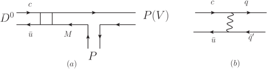
Figure 1: Annihilation diagram in the pole-dominance model

The weak matrix elements are evaluated in the vacuum insertion approximation$\!{}^{{\bf?}}$,

$$\langle M|\mathcal{H}|D\rangle = \frac{G_{F}}{\sqrt{2}}V_{CKM}a_{A,E}\langle M|\bar{q}_{1}\gamma_{\mu}(1-\gamma_{5})q_{2}|0\rangle\langle 0|\bar{q}_{3}\gamma^{\mu}(1-\gamma_{5})c|D\rangle$$ (5)

$$= \frac{G_{F}}{\sqrt{2}}V_{CKM}a_{A,E}f_{M}f_{D}m_{D}^{2},$$

where the effective coefficients $a_{A}$ and $a_{E}$ correspond to $W$-annihilation and $W$-exchange amplitudes respectively. Strong phases relative to the emission diagrams are also considered in these coefficients.

For the $PV$ modes, the effective strong coupling constants are defined through the Lagrangian

$$\mathcal{L}_{VPP}=ig_{VPP}V^{\mu}(P_{1}{\partial}_{\mu}P_{2}-P_{2}{\partial}_{\mu}P_{1}),$$ (6)

where $g_{VPP}$ is dimensionless and obtained from experiments. By inserting the propagator of the intermediate state $M$, the annihilation amplitudes are

$$\langle PV|\mathcal{H}_{eff}|D\rangle=\frac{G_{F}}{\sqrt{2}}V_{CKM}a_{A,E}f_{M}f_{D}m_{D}^{2}\frac{1}{m_{D}^{2}-m_{M}^{2}}g_{VPM}2(\varepsilon^{*}\cdot p_{D}).$$ (7)

As for the $PP$ modes, the intermediate mesons are scalar particles. The effective strong coupling constants are described by

$$\mathcal{L}_{SPP}=-g_{SPP}m_{S}SPP.$$ (8)

However, the decay constants of scalar mesons are very small, which is shown in the following relation

$$\frac{f_{S}}{\bar{f}_{S}}=\frac{m_{2}(\mu)-m_{1}(\mu)}{m_{S}},$$ (9)

where $f_{S}$ is the vector decay constant used in the pole model, $\bar{f}_{S}$ is the scale-independent scalar decay constant, $m_{1,2}$ are the running current quark mass, and $m_{S}$ is the mass of scalar meson. Therefore, the scalar pole contribution is very small, resulting in little resonant effect of annihilation type contributions in the $PP$ modes. On the contrary, large annihilation contributions are given in the $PV$ modes by relative large decay constants of intermediate pseudoscalar mesons.

3 Numerical results and discussions

In this method, only the effective Wilson coefficients with relative strong phases are free parameters, which are chosen to obtain the suitable results consistent with experimental data. For $PP$ modes,

$$a_{1} = 0.94\pm 0.10,~{}~{}~{}~{}~{}~{}~{}~{}~{}~{}~{}~{}~{}~{}~{}~{}~{}~{}a_{2}=(0.65\pm 0.10)e^{i(142\pm 10)^{\circ}},$$

$$a_{A} = (0.20\pm 0.10)e^{i(300\pm 10)^{\circ}},~{}~{}a_{E}=(1.7\pm 0.1)e^{i(90\pm 10)^{\circ}}.$$ (10)

For $PV$ modes,

$$a_{1}^{PV} = 1.32\pm 0.10,~{}~{}~{}~{}~{}~{}~{}~{}~{}~{}~{}~{}~{}~{}~{}~{}~{}a_{2}^{PV}=(0.75\pm 0.10)e^{i(160\pm 10)^{\circ}},$$

$$a_{A}^{PV} = (0.12\pm 0.10)e^{i(345\pm 10)^{\circ}},~{}~{}a_{E}^{PV}=(0.62\pm 0.10)e^{i(238\pm 10)^{\circ}}.$$ (11)

All the predictions of the 100 channels are shown in the tables of ref.$\!{}^{{\bf?}}$. The prediction of branching ratio of the pure annihilation process $D_{s}^{+}\to\pi^{+}\pi^{0}$ vanishes in the pole model within the isospin symmetry. It is also zero in the diagrammatic approach in the flavor SU(3) symmetry. Simply, two pions can form an isospin 0,1,2 state, but 0 is ruled out because of charged final states, and isospin-2 is forbidden for the leading order $\Delta C=1$ weak decay. The only left s-wave isospin-1 sate is forbidden by Bose-Einstein statics. In the pole model language, $G$ parity is violated in the isospin-1 case. Therefore, no annihilation amplitude contributes to this mode.

The theoretical analysis in the $\eta-\eta^{\prime}$ sector is kind of complicated. The predictions with $\eta^{\prime}$ in the final state are always smaller in this hybrid method than those case of $\eta$ due to the smaller phase space. However, it is opposite by experiments in some modes, such as $D_{s}^{+}\to\pi^{+}\eta(\eta^{\prime})$, $D^{0}\to\bar{K}^{0}\eta(\eta^{\prime})$. This may be the effects of SU(3) flavor symmetry breaking for $\eta_{q}$ and $\eta_{s}$, the error mixing angle between $\eta$ and $\eta^{\prime}$ , inelastic final state interaction, or the two gluon anomaly mostly associated to the $\eta^{\prime}$, etc.. The mode of $D_{s}^{+}\to\rho^{+}\eta(\eta^{\prime})$ is similar with the above two cases, the opposite ratio of $\eta$ over $\eta^{\prime}$ between theoretical prediction and the data. But this is a puzzle by experiment measurement, which is taken more than ten years ago $\!{}^{{\bf?}}$. As is questioned by PDG $\!{}^{{\bf?}}$, this branching ratio of $(12.5\pm 2.2)\%$ considerably exceeds the recent inclusive $\eta^{\prime}$ fraction of $(11.7\pm 1.8)\%$.

Recently, model independent diagrammatic approach is used to analyze the charm decays $\!{}^{{\bf?}}$. All two-body hadronic decays of $D$ mesons can be expressed in terms of some distinct topological diagrams within the SU(3) flavor symmetry, by extracting the topological amplitudes from the data $\!{}^{{\bf?}}$. Since the recent measurements of $D_{s}^{+}\to\pi^{+}\rho^{0}$ $\!{}^{{\bf?}}$ and $D_{s}^{+}\to\pi^{+}\omega$ $\!{}^{{\bf?}}$ give a strong constraint on the $W-$annihilation amplitudes, one cannot find a nice fit for $A_{P}$ and $A_{V}$ in the diagrammatic approach to the data with $D_{s}^{+}\to\bar{K}^{*0}K^{+},\bar{K}^{0}K^{*+}$ simultaneously. Compared to the calculations in the model-independent diagrammatic approach $\!{}^{{\bf?}}$, our hybrid method gives more predictions for the $PV$ modes in which the predictions are consistent with the experimental data. It is questioned that the measurement of $Br(D_{s}^{+}\to\bar{K}^{0}K^{*+})=(5.4\pm 1.2)\%$,$\!{}^{{\bf?}}$ which was taken two decades ago, was overestimated. Since $|C_{V}|<|C_{P}|$ and $A_{V}\approx A_{P}$ as a consequence of very small rate of $D_{s}^{+}\to\pi^{+}\rho^{0}$, it is expected that $Br(D_{s}^{+}\to\bar{K}^{0}K^{*+})<Br(D_{s}^{+}\to\bar{K}^{*0}K^{+})=(3.90\pm 0.23)\%$. Our result in the hybrid method also agrees with this argument.

As an application of the diagrammatic approach, the mixing parameters $x=(m_{1}-m_{2})/\Gamma$ and $y=(\Gamma_{1}-\Gamma_{2})/\Gamma$ in the $D^{0}-\bar{D}^{0}$ mixing are evaluated from the long distance contributions of the $PP$ and $VP$ modes $\!{}^{{\bf?}}$. The global fit and predictions in the diagrammatic approach are done in the SU(3) symmetry limit. However, as we know, the nonzero values of $x$ and $y$ come from the SU(3) breaking effect. Part of the flavor SU(3) breaking effects are considered in the factorization method and in the pole model. Therefore, our hybrid method takes its advantage in the analysis of $D^{0}-\bar{D}^{0}$ mixing.

References

References

- [1] Y. -Y. Keum, H. -n. Li, A. I. Sanda, Phys. Lett. B504, 6-14 (2001) [hep-ph/0004004]; Y. Y. Keum, H. -N. Li, A. I. Sanda, Phys. Rev. D63, 054008 (2001) [hep-ph/0004173]; C. -D. Lu, K. Ukai, M. -Z. Yang, Phys. Rev. D63, 074009 (2001) [hep-ph/0004213]; C. -D. Lu, M. -Z. Yang, Eur. Phys. J. C23, 275-287 (2002) [hep-ph/0011238].
- [2] M. Beneke, G. Buchalla, M. Neubert, C. T. Sachrajda, Phys. Rev. Lett. 83, 1914-1917 (1999) [hep-ph/9905312]; M. Beneke, G. Buchalla, M. Neubert, C. T. Sachrajda, Nucl. Phys. B591, 313-418 (2000) [hep-ph/0006124].
- [3] C. W. Bauer, D. Pirjol, I. W. Stewart, Phys. Rev. Lett. 87, 201806 (2001) [hep-ph/0107002]; C. W. Bauer, D. Pirjol, I. W. Stewart, Phys. Rev. D65, 054022 (2002) [hep-ph/0109045].
- [4] M. Wirbel, B. Stech, M. Bauer, Z. Phys. C29, 637 (1985); M. Bauer, B. Stech, M. Wirbel, Z. Phys. C34, 103 (1987).
- [5] H. -Y. Cheng, Phys. Lett. B335, 428-435 (1994) [hep-ph/9406262]; H. -Y. Cheng, Z. Phys. C69, 647-654 (1996) [hep-ph/9503219].
- [6] J. J. Sakurai, Phys. Rev. 156, 1508 (1967).
- [7] A. K. Das, V. S. Mathur, Mod. Phys. Lett. A8, 2079-2086 (1993) [hep-ph/9301279]; P. F. Bedaque, A. K. Das, V. S. Mathur, Phys. Rev. D49, 269-274 (1994) [hep-ph/9307296];
- [8] G. Kramer, C. -D. Lu, Int. J. Mod. Phys. A13, 3361-3384 (1998) [hep-ph/9707304].
- [9] Y. Fusheng, X. -X. Wang, C. -D. Lu, [arXiv:1101.4714].
- [10] T. Feldmann, P. Kroll, B. Stech, Phys. Rev. D58, 114006 (1998). [hep-ph/9802409].
- [11] C. P. Jessop et al. [CLEO Collaboration], Phys. Rev. D58, 052002 (1998) [hep-ex/9801010].
- [12] K. Nakamura et al. [ Particle Data Group Collaboration ], J. Phys. G G37, 075021 (2010).
- [13] J. L. Rosner, Phys. Rev. D60, 114026 (1999) [hep-ph/9905366].
- [14] H. -Y. Cheng, C. -W. Chiang, Phys. Rev. D81, 074021 (2010) [arXiv:1001.0987 [hep-ph]].
- [15] B. Aubert et al. [BABAR Collaboration], Phys. Rev. D79, 032003 (2009), arXiv:0808.0971 [hep-ex].
- [16] J. Y. Ge et al. [CLEO Collaboration], Phys. Rev. D80, 051102 (2009). [arXiv:0906.2138 [hep-ex]].
- [17] W. Y. Chen et al. [CLEO Collaboration ], Phys. Lett. B226, 192 (1989).
- [18] H. Y. Cheng and C. W. Chiang, Phys. Rev. D 81 (2010) 114020 arXiv:1005.1106 [hep-ph].