Computation of static Heisenberg chain correlators: Control over length and temperature dependence

Abstract

We communicate results on correlation functions for the spin-1/2 Heisenberg chain in two particularly important cases: (a) for the infinite chain at arbitrary finite temperature $T$, and (b) for finite chains of arbitrary length $L$ in the ground state. In both cases we present explicit formulas expressing the short-range correlators in a range of up to seven lattice sites in terms of a single function $\omega$ encoding the dependence of the correlators on $T$ ($L$). These formulas allow us to obtain accurate numerical values for the correlators and derived quantities like the entanglement entropy. By calculating the low $T$ (large $L$) asymptotics of $\omega$ we show that the asymptotics of the static correlation functions at any finite distance are $T^{2}$ ($1/L^{2}$) terms. We obtain exact and explicit formulas for the coefficients of the leading order terms for up to eight lattice sites.

Until about ten years ago it was widely believed that it would be practically impossible to calculate the lattice correlation functions of the Heisenberg chain explicitly, despite the fact that its Hamiltonian

$${\cal H}_{N}=J\sum_{j=1}^{L}\vec{\sigma}_{j}\vec{\sigma}_{j+1}$$ (1)

is one of the best known among those integrable lattice systems whose spectrum can be exactly calculated by means of the Bethe ansatz Bethe (1931). Starting from about the year 2000, however, our understanding of the model has changed profoundly.

The recent progress is due to several different but related methods, like the representation theory of quantum algebras, the algebraic Bethe ansatz, or the advent of new functional equations, which first of all led to the derivation of multiple integral representations Jimbo et al. (1992); *JiMi96; *KMT99b; *GKS04a for the elements of the density matrix. In a series of works Boos and Korepin (2001); *BKS03; *BKS04c; Boos et al. (2005) it was then shown that the correlation functions of an inhomogeneous version of the model can be represented by algebraic expressions of a single function of two variables.

An exponential formula for the reduced density matrix was obtained in Boos et al. (2006); *BJMST06. This formula will be of particular importance below, since it is also valid for finite temperature or finite length as was conjectured in Boos et al. (2006); *DGHK07. In Boos et al. (2007); *BJMST08a a fermionic structure on the space of local operators was identified from which a generating function of all local correlation functions was obtained Jimbo et al. (2009) for a very general inhomogenous vertex model including the finite temperature and the finite length Heisenberg chain as special cases. Even in this most general situation the inhomogeneous correlation functions depend on only two functions Jimbo et al. (2009); Boos and Göhmann (2009). Apart from these important theoretical findings many results for the ground state correlation functions in the thermodynamic limit, but also a number of finite temperature or finite length correlation functions were obtained explicitly, see e.g. Kitanine et al. (2005); *TGK10a and the references therein.

The aim of this paper is twofold. First, we present recent exact results for the temperature and size dependence of two-point correlation functions. Of particular interest are system parameters $T$ and $L$ in the regime of conformal field theory (CFT) and their influence on short-ranged correlators that are –strictly speaking– outside the domain of CFT. Furthermore, we present results for the entanglement entropy of sub-segments of an infinitely long chain in the entire temperature window from 0 to $\infty$. Second, we intend to explain the necessary computations in the light of a recent understanding of the subject Aufgebauer (2011) based on ‘discrete functional equations’ which we believe is physically most natural.

All information about the correlation functions of operators acting on $n$ successive sites of the chain are encoded in the reduced density matrix $D_{n}$. The matrix elements of $D_{n}$ are denoted by $D_{\sigma_{1},...,\sigma_{n}}^{\mu_{1},...,\mu_{n}}$ and correspond to the expectation values of operators $|\sigma_{1},...,\sigma_{n}\rangle\langle\mu_{1},...,\mu_{n}|$.

A quantum mechanical system at finite temperature $T$ may be viewed as a classical statistical system on a cylinder of circumference $\beta=1/T$. In this way, the density matrix $D_{n}$ on $n$ successive sites for temperature $T$ is obtained in a suitable limit of the six-vertex model density matrix on a rectangular lattice of unbounded width and finite height $N$. Each row corresponds to an imaginary time slice of height $\tau=\beta/N$, the continuous time limit is obtained in the Trotter limit $N\to\infty$. For our purposes it is convenient to have independent heights $\tau_{1},...,\tau_{N}$ (resp. spectral parameters $\epsilon_{1}$,… $\epsilon_{N}$ placed on the horizontal lines) under suitable conditions like $\tau_{j}={\cal O}(1/N)$ and $\sum_{j}\tau_{j}=\beta$.

We introduce independent spectral parameters $x_{1},...,x_{n}$ on the vertical lines corresponding to the $n$ sites picked for the definition of $D_{n}$. The density matrix of the generalized problem now depends on the ${x_{j}}$’s and is denoted by $D_{n}(x_{1},...,x_{n})$ with matrix elements $D_{\sigma_{1},...,\sigma_{n}}^{\mu_{1},...,\mu_{n}}(x_{1},...,x_{n})$. The full functional dependence will be solved, the subsequent specialization of the arguments yields the physically interesting data. The reason behind the success of this solution strategy is the analyticity of the object as a function of the spectral parameters $x$. This is a consequence of the integrabilty of the system: the eigenstates of the column-to-column transfer matrices $T(x)$ do not depend on $x$ and hence the eigenvalues and other objects as functions of $x$ do not show the otherwise unavoidable root singularities.

As an example of this solution strategy we like to note results for the leading eigenvalue $\Lambda(x)$ of the transfer matrix $T(x)$ which will be of use below

$$\log\Lambda(x)=e_{0}(x)+\frac{1}{2\pi}\int_{{\cal C}}\frac{\log(1+a(y))}{(x-y-{\rm i})(x-y)}dy.$$ (2)

Here, ${\cal C}$ is a narrow closed contour around the real axis, $e_{0}$ is some elementary function containing the $\epsilon_{j}$-parameters. The auxiliary function $a(x)$ satisfies the non-linear integral equation

$$\log a(x)=a_{0}(x)-\frac{1}{\pi}\int_{{\cal C}}\frac{\log(1+a(y))}{1+(x-y)^{2}}dy,$$ (3)

where $a_{0}(x)$ is an elementary function of $x$ and the $\epsilon_{j}$, which for finite temperature, in the Trotter limit $N\to\infty$, takes the form $a_{0}(x)=2J\beta/(x(x+{\rm i}))$. For the ground-state and finite size it is simply $a_{0}(x)=L\log\frac{x-{\rm i}/2}{x+{\rm i}/2}$.

The program of calculating the functional dependence of $D_{n}(x_{1},...,x_{n})$ is well understood in the case of zero temperature. For $T=0$ (i.e. $\beta=\infty$) the object $D_{n}(x_{1},...,x_{n})$ satisfies non-trivial linear functional equations in all arguments. The most important equation, the ‘rqKZ’-equation reads for instance

$$\mspace{-6.0mu}D_{n}(x_{1},...,x_{n-1},x_{n}-1)=A(x_{1},...,x_{n})D_{n}(x_{1},...,x_{n})$$ (4)

where $A$ is a linear operator Boos et al. (2005) acting in the space of density matrices and the $x_{j}$ may take any value from the complex plane. The action of $A$ on $D_{n}$ is of the following type

$$(AD)_{\vec{\sigma}}^{\vec{\mu}}=\sum_{\vec{\sigma}^{\prime},\vec{\mu}^{\prime}}A_{\vec{\sigma},\vec{\mu}^{\prime}}^{\vec{\mu},\vec{\sigma}^{\prime}}D_{\vec{\sigma}^{\prime}}^{\vec{\mu}^{\prime}}$$ (5)

The functional equations can be solved for the analytical function $D$. The uniqueness of the solution for $T=0$ is guaranteed by the asymptotic behaviour for $x_{j}\to\infty$. The finding of Boos et al. (2005) is striking, a two-point nearest neighbour function $\omega(x_{1},x_{2}):=$ $6$ tr $D_{2}(x_{1},x_{2})S_{1}^{z}S_{2}^{z}$ and a set of ‘structure constants’ $f_{n,I,J}$ determine the density matrix $D_{n}$ for arbitrary $n$

$$\mspace{-9.0mu}D_{n}=\sum_{m=0}^{[n/2]}\sum_{I,J}\left(\prod_{p=1}^{m}\omega(x_{I_{p}},x_{J_{p}})\right)f_{n,I,J}(x_{1},x_{2},...,x_{n})$$ (6)

The summation labels $I$ and $J$ are $m$-tuples of integers such that $I\cap J=\emptyset$ and $I_{1}<\dots<I_{m},\,1\leq I_{p}<J_{p}\leq n$. The structure coefficients $f_{n,I,J}(x_{1},x_{2},...,x_{n})$ are matrices with elementary rational functions of the arguments $x_{1},x_{2},...,x_{n}$ as entries. For details see Boos et al. (2005).

At zero temperature the computation of the correlation functions employed two important facts: (i) the functional equation (4) is satisfied for continuous arguments, and (ii) $D_{n}(x_{1},...,x_{n})$ depends on the arguments only via the differences $x_{j}-x_{i}$. This is fundamentally different for finite temperature, i.e. finite Trotter number $N$. The main problem is that (4) no longer holds: on the r.h.s. of (4) untreatable ‘correction terms’ appear, a serious obstacle so far for treating $T>0$.

At this point, the computation of the density matrix for finite Trotter number $N$ on the basis of functional equations looks unfeasable. However, for the above six-vertex model with $N$ many rows carrying spectral parameters $\epsilon_{1},...,\epsilon_{N}$ we find Aufgebauer (2011) a discrete version of functional equations. In detail:

(I) Equation (4) ‘rqKZ’ holds literally (!) if we restrict $x_{n}$ to the set $\{\epsilon_{1},...,\epsilon_{N}\}$.
(II) A reduction takes place in the limit of large spectral parameter $x_{n}$, i.e. $D_{n}(x_{1},...,x_{n})\to D_{n-1}(x_{1},...,x_{n-1})\otimes D_{1}$ where $D_{1}$ is a single site density matrix of a paramagnetic spin. For zero magnetic field this is $D_{1}=\frac{1}{2}$id.
(III) Analyticity properties:

$$D_{\sigma_{1},...,\sigma_{n}}^{\mu_{1},...,\mu_{n}}(x_{1},...,x_{n})=\frac{P_{\sigma_{1},...,\sigma_{n}}^{\mu_{1},...,\mu_{n}}(x_{1},...,x_{n})}{\Lambda(x_{1})\cdot...\cdot\Lambda(x_{n})}$$ (7)

where $P_{\sigma_{1},...,\sigma_{n}}^{\mu_{1},...,\mu_{n}}(x_{1},...,x_{n})$ is an $n$-variate polynomial of degree $N$ in the variables $x_{1},...,x_{n}$ and $\Lambda(x)$ is the largest eigenvalue of the transfer matrix $T(x)$ obtained from (2).

The computational problem consists in finding the polynomials $P_{\sigma_{1},...,\sigma_{n}}^{\mu_{1},...,\mu_{n}}(x_{1},...,x_{n})$. We have proved Aufgebauer (2011) that the above equations have a unique solution. Hence any expression (or ansatz) for $D_{n}(x_{1},...,x_{n})$ exhibiting the above listed properties realizes the solution.

We find that (I) is satisfied by (6) like in Boos et al. (2005) with the same structure coefficients $f_{n,I,J}$ provided that $\omega(x_{1},x_{2})$ is a symmetric function satisfying the ‘discrete functional equation’ (see Boos and Göhmann (2009) for the most general case)

$$\frac{\omega(x_{1},x_{2})}{x^{2}-1}+\frac{\omega(x_{1},x_{2}-1)}{x(x+2)}=\frac{3}{2(x^{2}-1)x(x+2)}$$ (8)

where $x:=x_{1}-x_{2}$, $x_{1}$ is arbitrary and $x_{2}\in\{\epsilon_{1},...,\epsilon_{N}\}$. The asymptotics (II) is satisfied if $\omega(x_{1},x_{2})\to 0$ for $x_{1}\to\infty$ or $x_{2}\to\infty$. Condition (III) is satisfied if $\omega$ is a polynomial (of degree $N-1$) divided by $\Lambda(x_{1})\Lambda(x_{2})$. These conditions for $\omega$ characterize a unique function. It is relatively straightforward to see that the conditions for $\omega$ are satisfied by the following expressions

$$\omega(x_{1},x_{2}) :=\frac{1}{2}+\frac{1}{2}((x_{1}-x_{2})^{2}-1)\psi({\rm i}x_{1},{\rm i}x_{2})$$

$$\psi(x_{1},x_{2}) :=\frac{1}{\pi}\int_{{\cal C}}\frac{dy}{1+a(y)}\frac{G(y,x_{1})}{(y-x_{2})(y-x_{2}-{\rm i})}$$ (9)

where the function $G$ satisfies the linear integral equation

$$G(x,x_{1})=\\ \mspace{-9.0mu}-\frac{1}{(x-x_{1})(x-x_{1}-{\rm i})}+\int_{{\cal C}}\frac{dy/\pi}{1+a(y)}\frac{G(y,x_{1})}{1+(x-y)^{2}}$$ (10)

and the function $a(x)$ was introduced in (3).

Note that the expression in (6) contains rational functions as prefactors. The poles of these coefficients are cancelled by zeros appearing due to the pairwise cancellation of terms in the sum. Consequently, the only poles on the r.h.s. of (6) are those occurring in the product ${\Lambda(x_{1})\cdot...\cdot\Lambda(x_{n})}$. Hence, also (III) is satisfied.

Finite temperature. The coefficients in (6) neither depend on $N$ nor on the parameters $\epsilon_{j}$. These only enter in $\omega$ via the dependence of $a$ and $G$ on them. Therefore, taking the Trotter limit $N\to\infty$ is easy.

Figure 1: Depiction of two-point correlators $\langle\sigma_{1}^{z}\sigma_{n}^{z}\rangle$ for different point separations $n$ in dependence on $J/T$ for antiferromagnetic (ferromagnetic) exchange to the right (left) of 0.

The evaluation of the correlation function consists in numerically solving (3) for $a(x)$. Then (10) is solved for $G$ and eventually $\omega$ is calculated from (9). The definition of the coefficients in (6) may be found in Boos et al. (2005), but an efficient computation is due to Sato et al. (2005); *Takahashi11. Here we use their results for density matrices $D_{n}$ with $n$ up to 7 sites, and combine this with the finite temperature results for the function $\omega$. The formulas for $D_{n}(x_{1},...,x_{n})$ allow for taking the homogeneous limit $x_{1}=...=x_{n}=0$ and yield simple algebraic expressions involving $\omega$ and its derivatives.

Just as an illustration of the explicit expressions we like to show formulas for the 2-point correlation functions obtained from $D_{n}$ for $n=2,3,4$

$$\langle\sigma_{1}^{z}\sigma_{2}^{z}\rangle =\frac{2}{3}{(0,0)},\ \langle\sigma_{1}^{z}\sigma_{3}^{z}\rangle=\frac{2}{3}{(0,0)}+\frac{2}{3}{(1,1)}-\frac{1}{3}{(2,0)}$$

$$\langle\sigma_{1}^{z}\sigma_{4}^{z}\rangle ={(0,0)}\left[\frac{2}{3}+\frac{4}{3}{(1,1)}+\frac{2}{9}{(2,2)}-\frac{4}{27}{(3,1)}\right]$$

$$\mspace{-18.0mu}-{(1,0)}\left[\frac{4}{3}{(1,0)}+\frac{4}{9}{(2,1)}-\frac{4}{27}{(3,0)}\right]-\frac{1}{9}{(3,1)}$$

$$\mspace{-18.0mu}+\left[4{(1,1)}-{2}{(2,0)}\right]\left[\frac{1}{3}+\frac{1}{9}{(2,0)}\right]+\frac{1}{6}{(2,2)}$$ (11)

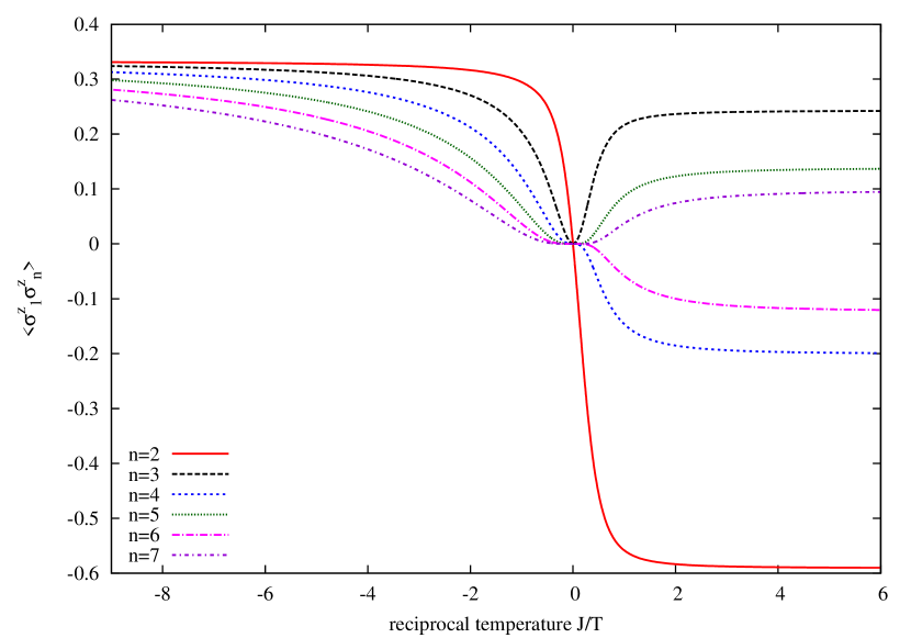
where $(j,k):=\partial^{j}_{1}\partial^{k}_{2}\omega(x_{1},x_{2})|_{x_{1}=x_{2}=0}$. We derived similar formulas for the cases $n=5,...,8$ but these are by far too long to be shown here. The correlators $\langle\sigma_{1}^{z}\sigma_{n}^{z}\rangle$ are analytic functions of $J/T$ along the entire real axis with zero of $(n-1)$th order at $J/T=0$. In Fig. 1 we show the results for the antiferromagnetic chain: data at negative values of $J/T$ correspond to results for the ferromagnetic chain at $|J/T|$. In the ferromagnetic case the correlations are strictly positive, in the antiferromagnetic case, the correlations are negative (positive) for even (odd) $n$.

In Crampé et al. (2010) the low-temperature behaviour of $\omega(x_{1},x_{2})$ was calculated with the result

$$\omega=\omega_{0}+\frac{T^{2}}{24J^{2}}\left(1-(x_{1}-x_{2})^{2}\right)\cos(\pi(x_{1}+x_{2})),$$ (12)

where $\omega_{0}$ denotes the $T=0$ limit of $\omega$ in the thermodynamic limit. From this expansion and (11) we obtain explicit results for the correlations like

$$\mspace{-9.0mu}\langle\sigma_{1}^{z}\sigma_{2}^{z}\rangle \simeq\frac{1}{3}-\frac{4}{3}\ln 2+\frac{1}{36}(T/J)^{2}$$

$$\mspace{-9.0mu}\langle\sigma_{1}^{z}\sigma_{3}^{z}\rangle \simeq\frac{1}{3}-\frac{16}{3}\ln 2+3\zeta(3)+\left(\frac{1}{9}-\frac{\pi^{2}}{72}\right)(T/J)^{2}$$ (13)

Similar but more lengthy expressions up to $\langle\sigma_{1}^{z}\sigma_{8}^{z}\rangle$ have been derived. These results can be written in the following form

$$\langle\sigma_{1}^{z}\sigma_{1+r}^{z}\rangle\simeq\langle\sigma_{1}^{z}\sigma_{1+r}^{z}\rangle_{0}(1-\gamma_{r}(T/J)^{2})$$ (14)

where explicit numbers for $\gamma_{r}$ are given in table 1.

1	2	3	4	5	6	7
0.0470	0.1070	0.3268	0.5014	0.9013	1.1957	1.7761
1.1283	0.6419	0.8714	0.7521	0.8652	0.7971	0.8699

Table 1: The low-temperature expansion coefficients $\gamma_{r}$ of the correlations $\langle\sigma_{1}^{z}\sigma_{1+r}^{z}\rangle$ for $r=1,...,7$ (2nd row) and the ratio of $\gamma_{r}$ with the CFT prediction $\gamma_{r}^{CFT}=r^{2}/24$ (3rd row).

For a (primary) field with scaling dimension $x$ the two-point correlator at distance $r$ is given by

$$C_{r}(T)=C\biggl{(}\frac{\pi T/{v}}{\sinh\pi rT/{v}}\biggr{)}^{2x}\simeq\frac{C}{r^{2x}}\left(1-\frac{x}{3}(\pi rT/v)^{2}\right)$$ (15)

where the sound velocity of the elementary excitations is $v=2\pi J$. For the spin-spin correlations we have to set $x=1/2$. Hence, the CFT prediction of the coefficient in (14) is $\gamma_{r}^{CFT}=r^{2}/24$. In table 1 results for the ratio $\gamma_{r}/\gamma_{r}^{CFT}$ are given. The values are of the order 1, but deviate significantly from 1 which we attribute to the simple form of the CFT prediction (14) which is strictly valid only for conformally invariant models without marginally irrelevant perturbations which exist in the isotropic Heisenberg chain. Also, it is likely that the sequence $\gamma_{r}/\gamma_{r}^{CFT}$ has two different accumulation points for even and odd $r$, respectively.

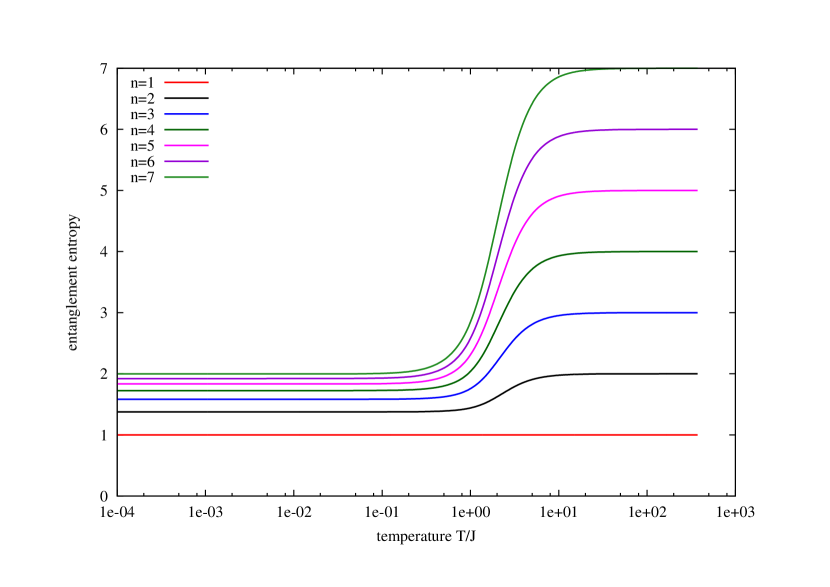
In Fig. 2 we show the entanglement entropies $S_{n}(T)$ for blocks of size $n$ for $n=1,...,7$. Note that we used the logarithm with base 2 (the total number of local states) in the definition of the entropy. Hence the high temperature asymptote of $S_{n}$ is identical to the length of the block $n$. The low-temperature limit scales with $1/3\log_{2}(n)$.

Figure 2: Depiction of the entanglement entropies of $D_{n}$ as functions of temperature.

Figure 3: Antiferromagnetic Heisenberg chain at $T=0$: Depiction of 2-point correlators $\langle\sigma_{1}^{z}\sigma_{n}^{z}\rangle$ in dependence on chain length $L$ for different point separations $n$. Solid lines are finite size fits.

Finite Size. Similar to (12) we find in the large $L$ limit

$$\omega=\omega_{0}+\frac{\pi^{2}}{6L^{2}}\left(1-(x_{1}-x_{2})^{2}\right)\cos(\pi(x_{1}+x_{2})).$$ (16)

For finite size, the physical density matrix is $D_{n}=D_{n}(1/2,...,1/2)$. Hence, all the above formulas for low $T$ turn into their counterparts for large $L$ if we replace $(2J/T)^{2}$ by $-L^{2}/\pi^{2}$ leading to

$$\langle\sigma_{1}^{z}\sigma_{1+r}^{z}\rangle\simeq\langle\sigma_{1}^{z}\sigma_{1+r}^{z}\rangle_{0}(1+4\gamma_{r}\pi^{2}/L^{2}).$$ (17)

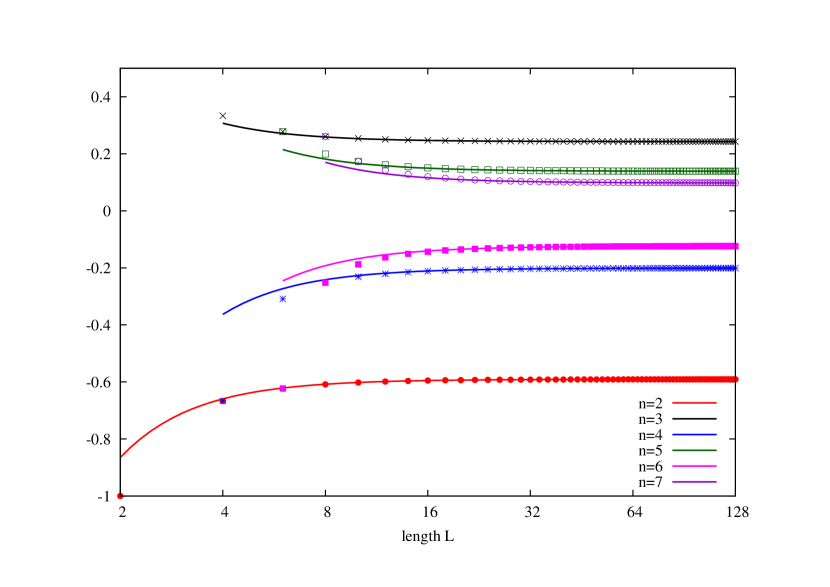
In contrast to finite temperature, finite size increases the correlations. In Fig. 3 we show data for chains of length $L$ up to $128$. Note that correlators $\langle\sigma_{1}^{z}\sigma_{n}^{z}\rangle$, $\langle\sigma_{1}^{z}\sigma_{m}^{z}\rangle$ for the same $L$ coincide if $n+m=L+2$.

In conclusion we have derived exact results for correlation functions of the Heisenberg spin chain for finite temperature $T$ (finite system size $L$). In the conformal regime of low $T$ (large $L$), the corrections to the ground-state results in the thermodynamic limit are additive $T^{2}$ ($L^{-2}$) terms. The exponents are universal and agree with CFT predictions. The coefficients for two-point correlators at strictly finite lattice separation are non-universal, but correspond precisely to those quantities that are of central interest in many, especially numerical approaches like the diagonalization of Hamiltonians or Monte-Carlo simulations. We also managed to derive multi-spin correlations and as an example we showed exact data for the entanglement entropy for arbitrary temperatures with smooth transitions from $T=0$ to $T=\infty$ with rather different dependence on the length of the chain segment. The central expression for all (static) correlation functions shows a remarkable structure, it is a sum of products of nearest-neighbour correlators. We also explained how the central expression for the correlations can be derived from a set of ‘discrete’ functional equations for the density matrix. We are convinced that this method is very powerful and applicable to other seminal models with higher spins or different symmetry groups as well.

Acknowledgments. M.T. acknowledges the Mercator professorship financed by DFG.

References

- Bethe (1931) H. Bethe, Z. Phys., 71, 205 (1931).
- Jimbo et al. (1992) M. Jimbo, K. Miki, T. Miwa, and A. Nakayashiki, Phys. Lett. A, 168, 256 (1992).
- Jimbo and Miwa (1996) M. Jimbo and T. Miwa, J. Phys. A, 29, 2923 (1996).
- Kitanine et al. (2000) N. Kitanine, J. M. Maillet, and V. Terras, Nucl. Phys. B, 567, 554 (2000).
- Göhmann et al. (2004) F. Göhmann, A. Klümper, and A. Seel, J. Phys. A, 37, 7625 (2004).
- Boos and Korepin (2001) H. E. Boos and V. E. Korepin, J. Phys. A, 34, 5311 (2001).
- Boos et al. (2003) H. E. Boos, V. E. Korepin, and F. A. Smirnov, Nucl. Phys. B, 658, 417 (2003).
- Boos et al. (2004) H. E. Boos, V. E. Korepin, and F. A. Smirnov, Moscow Math. J., 4, 593 (2004).
- Boos et al. (2005) H. Boos, M. Jimbo, T. Miwa, F. Smirnov, and Y. Takeyama, Algebra and Analysis, 17, 115 (2005).
- Boos et al. (2006) H. Boos, M. Jimbo, T. Miwa, F. Smirnov, and Y. Takeyama, Lett. Math. Phys., 75, 201 (2006a).
- Boos et al. (2006) H. Boos, M. Jimbo, T. Miwa, F. Smirnov, and Y. Takeyama, Ann. Henri Poincaré, 7, 1395 (2006b).
- Boos et al. (2006) H. Boos, F. Göhmann, A. Klümper, and J. Suzuki, J. Stat. Mech.: Theor. Exp., P04001 (2006c).
- Damerau et al. (2007) J. Damerau, F. Göhmann, N. P. Hasenclever, and A. Klümper, J. Phys. A, 40, 4439 (2007).
- Boos et al. (2007) H. Boos, M. Jimbo, T. Miwa, F. Smirnov, and Y. Takeyama, Comm. Math. Phys., 272, 263 (2007).
- Boos et al. (2009) H. Boos, M. Jimbo, T. Miwa, F. Smirnov, and Y. Takeyama, Comm. Math. Phys., 286, 875 (2009).
- Jimbo et al. (2009) M. Jimbo, T. Miwa, and F. Smirnov, J. Phys. A, 42, 304018 (2009).
- Boos and Göhmann (2009) H. Boos and F. Göhmann, J. Phys. A, 42, 315001 (2009).
- Kitanine et al. (2005) N. Kitanine, J. M. Maillet, N. A. Slavnov, and V. Terras, J. Stat. Mech.: Theor. Exp., L09002 (2005).
- Trippe et al. (2010) C. Trippe, F. Göhmann, and A. Klümper, Eur. Phys. J. B, 73, 253 (2010).
- Aufgebauer (2011) B. Aufgebauer, Berechnung der Korrelationsfunktionen des Heisenberg-Modells bei endlicher Temperatur mittels Funktionalgleichungen, Ph.D. thesis, Bergische Universität Wuppertal (2011).
- Sato et al. (2005) J. Sato, M. Shiroishi, and M. Takahashi, Nucl. Phys. B, 729, 441 (2005).
- Takahashi (2011) M. Takahashi, SIGMA, 7, 004 (2011).
- Crampé et al. (2010) N. Crampé, F. Göhmann, and A. Klümper, SIGMA, 6, 082 (2010).