Do quasar broad–line velocity widths add any information to virial black hole mass estimates?

Abstract

We examine how much information measured broad–line widths add to virial BH mass estimates for flux limited samples of quasars. We do this by comparing the BH masses estimates to those derived by randomly reassigning the quasar broad–line widths to different objects and re-calculating the BH mass.

For 9000 BH masses derived from the H $\beta$ line we find that the distributions of original and randomized BH masses in the $M_{\rm BH}$–redshift plane and the $M_{\rm BH}$–luminosity plane are formally identical. A 2D KS test does not find a difference at $>90$% confidence. For the Mg II line (32000 quasars) we do find very significant differences between the randomized and original BH masses, but the amplitude of the difference is still small. The difference for the C IV line (14000 quasars) is $2-3\sigma$ and again the amplitude of the difference is small. Subdividing the data into redshift and luminosity bins we find that the median absolute difference in BH mass between the original and randomized data is 0.025, 0.01 and 0.04 dex for H $\beta$, Mg II and C IV respectively. The maximum absolute difference is always $\leq 0.1$ dex.

We investigate whether our results are sensitive to corrections to Mg II virial masses, such as those suggested by Onken & Kollmeier (2008). These corrections do not influence our results, other than to reduce the significance of the difference between original and randomized BH masses to only $1-2\sigma$ for Mg II. Moreover, we demonstrate that the correlation between mass residuals and Eddington ratio discussed by Onken & Kollmeier are more directly attributable to the slope of the relation between H $\beta$ and Mg II line width.

The implication is that the measured quasar broad–line velocity widths provide little extra information, after allowing for the mean velocity width. In this case virial estimates are equivalent to $M_{\rm BH}\propto L^{\alpha}$, with $L/L_{\rm Edd}\propto L^{1-\alpha}$ (with $\alpha\simeq 0.5$). This leaves an unanswered question of why the accretion efficiency changes with luminosity in just the right way to keep the mean broad–line widths fixed as a function of luminosity.

1. Introduction

It is now clear that accretion onto super-massive black holes (BHs) plays a crucial role in the process of galaxy formation and evolution. These BHs lie at the center of all massive galaxies and are thought to influence galaxy evolution via powerful radiative (i.e. quasar mode) and mechanical (radio mode) feedback (e.g. Croton et al. 2006). The tight correlation between BH mass and the properties of the spheroidal component of their host galaxies (e.g. Tremaine et al. 2002) infers that the growth of both is closely related.

The fundamental observables of black holes are mass and spin. While spin is still elusive (only being inferred from very indirect means), there are now various approaches to the measurement of BH masses. The best constraint come from the BH at the centre of the Milky Way via stellar kinematics (e.g. Gillessen et al. 2009) and the BH in NGC 4258 via mega-maser orbits (Miyoshi et al. 1995). The masses of BHs in other local galaxies can be estimated by the impact of the BH on the motion of stars close to the nucleus, but model degeneracies remain (Gebhardt & Thomas 2009).

For type-1 AGN, where we see all the way to the active nucleus, the high velocity gas surrounding the BH gives us another probe of the BH potential. This is particularly powerful because it does not rely on spatially resolving the sphere of influence of the BH and because the the light from a quasar often overwhelms the light emanating from its host galaxy. As a result BH masses can be estimated in high redshift quasars. The disadvantage to this approach is that gas kinematics can be more complex than the effectively collisionless stars. Physical processes such as radiation pressure and outflows (e.g. Marconi et al. 2008) may cause potential biases in BH mass determinations, although recent work suggests that this is not serious (Netzer & Marziani 2010).

The approach to estimating BH masses using quasar broad emission lines relies on the assumption that the gas is largely in virial motion about the BH. If this is the case, we then require an estimate of the radius and velocity of the broad line region to estimate mass such that

$$M_{\rm BH}=\frac{f\sigma_{\rm BLR}^{2}R_{\rm BLR}}{G},$$ (1)

where $f$ is a geometric factor, $R_{\rm BLR}$ is the radius of the broad line region, $\sigma_{\rm BLR}^{2}$ is the velocity width of the line and $G$ is the gravitational constant. The only viable approach to measuring $R_{\rm BLR}$ is reverberation mapping (Blandford & McKee 1983). Evidence from multiple lines within the same objects is consistent with virial motion of the broad line region (Peterson & Wandel 1999). Reverberation mapping is limited to low redshift and low luminosity broad line objects (i.e. Seyfert 1s), largely because time-dilation and the scaling of $R_{\rm BLR}$ with luminosity (typically $R_{\rm BLR}\sim L^{0.5}$ if driven by photo-ionization) can increase by an order of magnitude or more the time lag between continuum and line variability. In order to make estimates of BH mass in higher redshift quasars the correlation between $R_{\rm BLR}$ and luminosity found via reverberation mapping (e.g. Kaspi et al. 2000) has been applied. Using the $R_{\rm BLR}-L$ relation and calibrating to the H $\beta$ emission line visible at low redshift, both the Mg II (McLure & Jarvis 2002) and C IV (Vestergaard et al. 2006) emission lines have been used for BH mass estimation. This approach, using the width of a broad optical or UV emission line and the $R_{\rm BLR}-L$ relation is generally termed the virial method. The power of such techniques is that they can be applied to large optical spectroscopic samples of quasars such as the Sloan Digital Sky Survey (SDSS; Schneider et al. 2007), 2dF QSO Redshift Survey (2QZ; Croom et al. 2004) and 2dF-SDSS LRG and QSO Survey (2SLAQ; Croom et al. 2009). It is then in principle possible to study properties such as mass functions (e.g. Vestergaard et al. 2008) or the clustering of quasars as a function of BH mass (e.g. Shen et al. 2009).

The above approaches give us great hope of characterizing the super-massive BH population over most of cosmic time. However, a number key issues have been raised. The C IV line in particular has been a subject of close scrutiny (e.g. Netzer et al. 2007; Baskin & Laor 2005) largely due to the strong asymmetries and absorption often seen in this line. However some authors argue that C IV can be used to provide a viable mass estimate (e.g. Vestergaard & Peterson 2006). This is because the asymmetries in C IV cause mass differences which are smaller than the relatively large scatter in the virial estimates. Vestergaard & Peterson also argue that for the handful of objects which have reverberation mapping of multiple lines (including C IV), these provide consistent BH mass estimates. Not withstanding these points, the C IV line is thought to be located much closer to the nucleus than H $\beta$ or Mg II so it is quite possible that different dynamics are in play in these two regimes.

More generally, one of the recent challenges to the virial method is the study of the dispersion in quasar broad line widths as a function of luminosity for Mg II and C IV by Fine et al. (2008) and Fine et al. (2010) respectively. The most striking result from this work is the small scatter in line widths for the most luminous quasars, which is less than 0.1 dex for both the Mg II and C IV lines. This implies a scatter of less than 0.2 dex in BH mass. Given that this scatter must include dispersion due to accretion rate variations, orientation effects, scatter in the $R_{\rm BLR}-L$ relation and observational uncertainty, it is hard to see how such a small scatter can be produced. This scatter is also smaller than the typical quoted uncertainties on virial BH mass estimates.

In this paper we consider the low scatter present in broad line velocity widths and address the question of how much information they actually provide concerning virial BH mass estimates. Our approach is to carry out a simple test of re-determining BH masses after randomly reassigning the broad-line velocity widths to different quasars. Throughout this paper we assume a flat cosmology with $H_{0}=70$km s^-1Mpc^-1, $\Omega_{\rm m}=0.3$ and $\Omega_{\Lambda}=0.7$.

2. Black hole masses

Figure 1.— The distribution of line width [$\log(v)$], bolometric luminosity [$\log(L_{\rm Bol})$] and redshift for the samples analysed in this paper. The H $\beta$ (black), Mg II (blue) and C IV (red) samples are shown separately. Contours are linearly spaced in 5 equal intervals. The lower left plot also shows the AGN with reverberation mapping used to calibrate virial relations [open squares; taken from vestergaard & Peterson (2006)] and the approximate flux limits of the SDSS (top), 2QZ (middle) and 2SLAQ (bottom) using the mean bolometric correction from the B-band given by McLure & Dunlop (2004). For the 2QZ and 2SLAQ surveys the edge of the locus of sources lies close to these limits, while for SDSS which is $i$-band limited the sources have greater scatter across the nominal survey limits. Mg II and C IV line widths have been corrected to match the FWHM measurements of the H $\beta$ lines assuming the lines are single Gaussians.

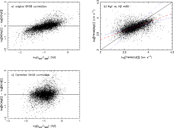
Figure 2.— a) The correlation between BH mass difference and Eddington ratio as given by OK08 using the data of Shen et al. (2008). b) The correlation between Mg II and H $\beta$ velocity width from the same data, which shows a gradient which deviates from 1-to-1 (black solid line). The OLS$(X|Y)$ and OLS$(Y|X)$ fits are shown by the blue dotted lines and the bi-sector of these is given by the red dashed line. c) The relation between mass difference and Eddington ratio after correcting the Mg II velocity.

The measurements of H $\beta$ broad line widths is taken from Shen et al. (2008), who use the fifth data release of the SDSS quasar survey (Schneider et al 2007). Shen et al. largely follow the procedure of McLure & Dunlop (2004), including their calibration of the virial BH mass estimator. This involves first fitting the underlying power–law continuum plus iron emission, which is then subtracted off. They then fit a double Gaussian to the emission line, constraining one component to be broad, and the other narrow. The FWHM of the line is then taken to be that of the broad Gaussian component.

For the Mg II and C IV emission line fits we use the results of Fine et al. (2008) and Fine et al. (2010) respectively. The main reason for using the Fine et al. data sets is that as well as using quasars from the SDSS, they also use spectra from the 2dF QSO Redshift Survey (2QZ; Croom et al. 2004) and the 2dF-SDSS LRG and QSO Survey (2SLAQ; Croom et al. 2009). This provides a larger dynamic range in luminosity at any given redshift. The line width measurements made by Fine et al. use the inter–percentile value (IPV) width (e.g. Whittle 1985). Continuum plus Fe II emission is first subtracted, and then a single Gaussian fitted. The IPV width is then measured over the range $\pm 1.5\times$ the Gaussian FWHM. The IPV approach has the advantages that it is doesn’t depend on a particular line shape, and as it is derived from the cumulative sum of flux in the line, easier quantification of the errors are possible (particularly incorporating the covariance due to continuum subtraction, which is generally not included in line fits). In the case of C IV Fine et al. (2010) also fit and subtract the contaminating He II and O III] at $\simeq 1600$Å. The virial BH mass estimates use the McLure & Dunlop (2004) and Vestergaard & Peterson (2006) calibrations for Mg II and C IV respectively. The distribution of redshift, bolometric luminosity and linewidth is shown is Fig. 1. The fainter 2QZ and 2SLAQ samples allow us to probe a broader range of luminosities than just the SDSS alone, similar to the work of Kollmeier et al. (2006) who also target faint AGN (limited to $R<21.5$).

The exact form of the virial relation and its calibration is not crucial in the analysis presented below. Our aim is to determine how much information the broad line velocity width contributes to distribution of measured black hole masses. To this end we perform the simple test of randomizing the measured velocities. That is, assigning the velocity width of one quasar to another. We do this without reference to an object’s redshift or luminosity (other than to only randomize H $\beta$ widths with other H $\beta$ widths, and similarly for Mg II and C IV), so that a quasar at the low luminosity and low redshift end of the sample could be given a width from a high redshift, high luminosity object. If the velocity widths are adding useful information to our black hole mass estimates, then the distribution of original black hole masses should be significantly different from the randomized black hole masses.

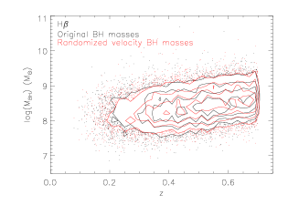
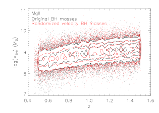
Figure 3.— The distribution of black hole mass estimates vs. redshift using the H $\beta$ (top left), Mg II (top right) and C IV (bottom left) lines. The black contours and points are the original BH masses (Shen et al. 2008 for H $\beta$  Fine et al., 2008 for Mg II and Fine et al. 2010 for C IV), while the red contours and points with the broad line velocities randomized. The contours are used in regions of high density and are spaced at five equal linear intervals, using the same levels for both black and red contours.

The work of Onken & Kollmeier (2008, OK08) suggested that Mg II based virial methods contain a bias which is a function of Eddington ratio. We also investigate whether such a bias influences our results presented below. OK08 present the bias as a mass difference [$M$(Mg II)-$M$(H $\beta$)] as a function of $L/L_{\rm Edd}$ (Fig. 2a). However, these are both derived quantities which are correlated in non-trivial ways. In terms of measured (rather than derived) quantities this bias is due to the relation between H $\beta$ and Mg II velocity width not having a gradient of 1 (see fig. 2b). OK08 define a matrix of corrections for the Mg II mass estimates. However, we find that a much more direct correction of the Mg II velocity widths also removes the bias. We find this correction by making an ordinary least squares (OLS) fit to FWHM(Mg II) vs. FWHM (H $\beta$) in both $(X|Y)$ and $(Y|X)$ and taking the bisector (red dashed line in Fig. 2b; Isobe et al. 1990). The resulting fit is

$$\log[{\rm FWHM(MgII)}]=1.70+0.54\log[{\rm FWHM(H\beta)}].$$ (2)

Applying this relation to correct the Mg II velocity widths results in an offset with respect to the original virial relation, which is corrected by using

$$\log\left(\frac{M_{\rm BH}}{M_{\odot}}\right) = 0.505+0.62\log\left(\frac{\lambda L_{\lambda}}{10^{44}\rm{ergs~{}s^{-1}}}\right)$$ (3)

$$+2\log\left(\frac{{\rm FWHM(MgII)_{\rm c}}}{{\rm km~{}s^{-1}}}\right)+1.278,$$

where the final term ($+1.278$) corrects the offset caused by the Mg II velocity correction. ${\rm FWHM(MgII)_{\rm c}}$ is the Mg II width corrected to match H $\beta$ using Eq. 2. The result of applying the above BH mass estimate, including the correction to Mg II velocities, is shown in Fig. 2c. It can be seen that this corrects the strong bias originally presented by OK08. Applying such a correction as part of our analysis has no impact on the result presented in this paper. Further details will be described below. A gradient in FWHM(Mg II) vs. FWHM (H $\beta$) which deviates from one also has more broad implications for the virial technique. Assuming that the H $\beta$ line is virialized and that the exponent for the velocity is 2 (as in Eq. 1), then the implied exponent for the Mg II velocities is $2/0.54\simeq 3.7$. This deviation from a naive virial relation is similar to the results of Wang et al. (2009) who look at the calibration of virial relations without the assumption that the exponent for the velocity is 2. It could be that the virial assumption is wrong for either H $\beta$ or Mg II or that the relative distribution of gas is markedly different. Infact, H $\beta$ is expected to be due to multiple components (e.g. Sulentic et al. 2006). Our lack of understanding of the differences between H $\beta$ and Mg II is a concern for the virial approach.

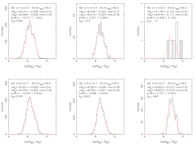
Figure 4.— The distribution of black hole mass estimates in different redshift and bolometric luminosity intervals for H $\beta$. We compare the original mass estimates ($M_{\rm O}$; black solid lines) to the randomized estimates ($M_{\rm R}$; red dashed lines). Mean masses are given for both, along with the difference in the mass and its significance.

3. Results

Table 1The results of a 2-D KS test comparing original and randomized BH masses in both the $M_{\rm BH}-z$ and $M_{\rm BH}-L$ planes.

Line	Test	NQ	$D_{\rm KS}$	$P(>D)$
H $\beta$ (SDSS)	$M_{\rm BH}-z$	8979	0.0194	2.18E-01
H $\beta$ (SDSS)	$M_{\rm BH}-L$	8979	0.0223	9.38E-02
Mg II (all)	$M_{\rm BH}-z$	32214	0.0290	2.94E-08
Mg II (all)	$M_{\rm BH}-L$	32214	0.0230	8.27E-06
Mg II (all, corrected)	$M_{\rm BH}-z$	32214	0.0280	7.32E-02
Mg II (all, corrected)	$M_{\rm BH}-L$	32214	0.0236	1.79E-01
Mg II (SDSS)	$M_{\rm BH}-z$	22910	0.0295	6.22E-06
Mg II (SDSS)	$M_{\rm BH}-L$	22910	0.0259	8.10E-05
Mg II (2QZ)	$M_{\rm BH}-z$	6784	0.0221	2.41E-01
Mg II (2QZ)	$M_{\rm BH}-L$	6784	0.0212	2.54E-01
Mg II (2SLAQ)	$M_{\rm BH}-z$	2491	0.0252	6.54E-01
Mg II (2SLAQ)	$M_{\rm BH}-L$	2491	0.0278	5.21E-01
C IV  (all)	$M_{\rm BH}-z$	13795	0.0213	3.30E-02
C IV  (all)	$M_{\rm BH}-L$	13795	0.0257	2.33E-03
C IV  (SDSS)	$M_{\rm BH}-z$	11861	0.0215	5.97E-02
C IV  (SDSS)	$M_{\rm BH}-L$	11861	0.0255	9.94E-03
C IV  (2QZ)	$M_{\rm BH}-z$	1593	0.0341	5.71E-01
C IV  (2QZ)	$M_{\rm BH}-L$	1593	0.0303	6.78E-01
C IV  (2SLAQ)	$M_{\rm BH}-z$	307	0.0642	7.48E-01
C IV  (2SLAQ)	$M_{\rm BH}-L$	307	0.0572	8.24E-01

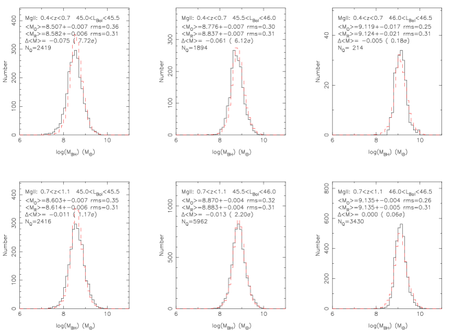
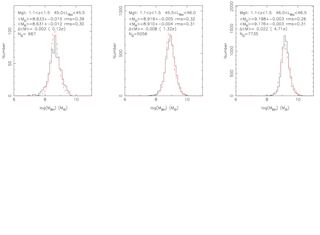
Figure 5.— The distribution of black hole mass estimates in different redshift and bolometric luminosity intervals for Mg II. We compare the original mass estimates ($M_{\rm O}$; black solid lines) to the randomized estimates ($M_{\rm R}$; red dashed lines). Mean masses are given for both, along with the difference in the mass and its significance.

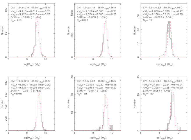
Figure 6.— The distribution of black hole mass estimates in different redshift and bolometric luminosity intervals for C IV. We compare the original mass estimates ($M_{\rm O}$; black solid lines) to the randomized estimates ($M_{\rm R}$; red dashed lines). Mean masses are given for both, along with the difference in the mass and its significance.

We first assess what the impact of randomization is on a single quasar by measuring the RMS of ($M_{\rm O}$-$M_{\rm R}$). We find RMSs of 0.54, 0.42 and 0.27 dex for H $\beta$, Mg II and C IV respectively. In comparison to this the quoted uncertainties on the virial estimators are typically 0.3-0.4 dex. Vestergaard & Peterson (2006) find a scatter of 0.43 and 0.33-0.43 dex for H $\beta$ and C IV respectively, while McLure & Dunlop (2004) find a scatter of 0.33 dex for the comparison between Mg II and H $\beta$ based mass estimates. This suggests that taking a mean velocity width to estimate a BH mass based simply on luminosity could be a useful approach, all be it, with some increase in the related error on BH mass.

The distribution of $M_{\rm BH}$ vs. redshift is shown in Fig. 3 for the H $\beta$, Mg II and C IV lines. The original distributions are shown in black and the distribution after randomizing the emission line velocity widths are shown in red. In all three cases the original and randomized black hole masses appear essentially indistinguishable. To examine whether there is a quantitative difference we perform a 2-D Kolmogorov–Smirnov (KS) test (Peacock 1983). We carry out these tests in both the $M_{\rm BH}-z$ and $M_{\rm BH}-L$ planes. To provide a robust estimate we generate 100 random realizations of the randomized BH masses and then take the median $D_{\rm KS}$ and probability, although taking a single realization does not significantly change our conclusions. Table 1 contains the results of the 2-D KS analysis. For the H $\beta$ line there is no significant difference between the original and randomized distributions of $M_{\rm BH}-z$ or $M_{\rm BH}-L$ (the null hypothesis that they are drawn from the same distribution is only rejected at the $\simeq 20$% and $\simeq 10$% level for $M_{\rm BH}-z$ or $M_{\rm BH}-L$ respectively). Applying this test to the Mg II mass estimates we find similar values of $D_{\rm KS}$, but due to the larger number of quasars the difference between the original and randomized BH masses is now highly significant. Careful inspection of Fig. 3 does show that the randomized Mg II BH masses have a slightly broader distribution at high redshift than the original BH masses. This could be due to intrinsic correlations of Mg II line width with redshift or luminosity (which indeed are seen by Fine et al. 2008). Alternatively, it could be driven by correlations of measurement errors with redshift or luminosity. Larger measurement errors will broaden the BH mass distribution, and if signal–to–noise is correlated with luminosity or redshift this will cause a difference between our original and randomized BH masses. If we apply corrections to the Mg II velocities as described in Sec. 2, then the significance of the difference in the distribution of original and randomized BH masses is reduced to only  1-2$\sigma$. However, to be conservative we will consider the Mg II mass estimates without this correction for the remainder of the paper. For the C IV line the derived $D_{\rm KS}$ values are again similar, and the significance of the difference is at the 2 ($M_{\rm BH}-z$) to $3\sigma$ ($M_{\rm BH}-L$) level.

It might be expected that a combination of the Eddington limit and the bright end of the BH mass function might naturally cause a narrowness in the distribution of velocity widths. To examine this we carry out the same analysis as above, but this time keeping each sample separate. The results are listed in Table 1. In the case of the 2SLAQ and 2QZ samples, there is no significant difference between the original and randomized BH masses.

Our second test is to measure the mean and RMS BH masses using each estimator in various redshift and bolometric luminosity bins. Again we calculate the values for the randomized sample from 100 realizations, although we calculate the error on the mean assuming a single random sample. The results of this analysis are presented in Figs. 4, 5 and 6. In all cases there is a good agreement between the original ($M_{\rm O}$) and randomized ($M_{\rm R}$) mass estimates. For H $\beta$ the difference in mean mass is always less than 0.1 dex (except for the $0.1<z<0.4$, $46<L_{\rm Bol}<46.5$ interval which only contains 12 quasars) and the median difference is $\simeq 0.02-0.03$ dex. Three $z-L_{\rm Bol}$ intervals have differences in the mean masses which are greater than $2\sigma$. The comparison of Mg II BH masses in Fig. 5 shows similar good agreement. The largest difference is 0.075 dex, and the median absolute difference is only 0.01 dex. Again, there are several intervals where the difference between the mean masses is significant. The C IV masses (Fig. 6) are consistent with the other emission lines. The maximum difference is 0.1 dex and the median is $0.03-0.05$ dex. Two of the intervals have significantly ($>2\sigma$) different means. Overall, while there are some significant differences in the mean $M_{\rm BH}$, there is impressive agreement between the original and randomized BH masses. Such agreement has a number of implications, which we will discuss below.

4. Discussion

The virial method makes use of the radius–luminosity relation derived from reverberation mapping, so that the only observables required are velocity width and luminosity. Thus we have

$$M_{\rm BH}=A\times L_{\lambda}^{\alpha}\times\sigma_{\rm BLR}^{2},$$ (4)

where $A$ is a normalizing constant, $L_{\lambda}$ is the monochromatic luminosity at some wavelength $\lambda$ near the emission line, $\alpha$ is $\simeq 0.5$ (e.g. Bentz et al. 2009) and $\sigma_{\rm BLR}$ is the width of the emission line. There are multiple stages required to make the connection between BH mass and the directly observable values. Starting with BH mass these are:

1. Black hole mass ($M_{\rm BH}$) and accretion rate ($L/L_{\rm Edd}$) give us bolometric luminosity, $L_{\rm Bol}$.

2. $L_{\rm Bol}$ combined with bolometric corrections and photometric errors give us $L_{\lambda}$, the first observable.

3. $L_{\rm Bol}$ (or possibly $L_{\rm UV}$) defines the radius of the broad line region $R_{\rm BLR}$.

4. $M_{\rm BH}$ and $R_{\rm BLR}$, together with the assumption of Keplerian orbits, gives us the velocity of the broad line gas, $V_{\rm BLR}$.

5. $V_{\rm BLR}$ together with non-virial motion, orientation effects and measurement errors give us $\sigma_{\rm BLR}$, the second observable.

An important point to note is that, apart from uncertainty in the bolometric correction and photometric errors, scatter or errors in each of these steps will increase the scatter in $\sigma_{\rm BLR}$ at a given luminosity. The measured uncertainties in virial relations are typically $0.3-0.4$ dex (Vestergaard & Peterson 2006), and these are only statistical errors and do not include contributions from systematic uncertainties in the reverberation mapping data, to which the virial relations are calibrated. The difference between the mean BH masses measured in our original and randomized samples was at most 0.1 dex, and typically 0.02 dex. This is much smaller than the uncertainties in the estimators themselves. Indeed to highlight this fact, we compare the SDSS Mg II BH masses calculated by Shen et al. (2008) and Fine et al. (2008). Although both use the same virial relation calibration, the difference in method (FWHM vs. IPV) results in a typical difference of the mean BH mass (in narrow redshift and luminosity bins) of $\simeq 0.25$ dex. This is an order of magnitude greater than the difference between our original and random estimates, although it is worth noting that the line measurement methods of these two works are somewhat different.

The above results suggest that assuming a mean velocity width and an RMS scatter about that mean would enable us to estimate the BH mass distribution to the same precision as we currently have using the individual measured line widths. This has a number of implications for the use of virial BH masses. One of the most common derived quantities is the accretion efficiency $L/L_{\rm Edd}$. As the velocity width adds little information, $L/L_{\rm Edd}\propto L^{1-\alpha}$, where $\alpha\simeq 0.5$. In a flux limited sample the most distant objects will be the most luminous and so will be found to have the highest efficiency.

We know that quasar broad emission line properties do correlate with various observables. The best known case being the Baldwin (1977) effect which correlates equivalent width with luminosity. Fine et al. (2008) finds that although the mean width of the Mg II line does not depend on luminosity, the dispersion of line widths does. There is a significantly broader distribution of line widths at faint luminosities. No doubt this contributes to the small but significant difference we do see between our original and randomized BH masses. In contrast, Fine et al. (2010) find no correlation between the dispersion in C IV width and luminosity (once corrected for measurement errors). The low overall dispersion in line width found ($<0.1$dex at high luminosity) by both these works naturally infers that in a flux limited sample quasar broad line widths cannot have a large impact on BH mass estimates. The small scatter and other observed properties (e.g. the presence of strong outflows indicated by broad absorption lines) may infer a problem with our assumption that the broad line gas is virialized. However, there are a number of observations which suggest that virialization is at least partially correct. The most compelling being the correlation between lag and line width (e.g. Peterson et al. 2004). Comparisons between broad line reverberation mapping masses and bulge velocity dispersion shows a correlation analogous to that observed in quiescent galaxies (Onken et al. 2004). Added to this, there is agreement between dynamical mass and reverberation masses for the few galaxies where measurements have been possible (Davies et al. 2006; Onken et al. 2007; Hicks & Malkan 2007).

The small impact of velocity width on BH masses is due to the limited dynamic range of velocity widths. Under assumption that the virial method is giving us real information concerning BH mass, the small range in velocity widths must be in part due to joint constraints from a steep BH mass function at high masses and the Eddington limit. Fine et al. (2008) examine this and find that some bias is possible, but that selection effects cannot on their own produce the narrowness of the velocity distribution for the most luminous quasars. A more robust examination would be to extend the approach of Schulze & Wisotzki (2010) to the larger SDSS, 2QZ and 2SLAQ samples, although this is outside the scope of the present paper. However, we do find that there is no significant difference between original and randomized BH masses when we test the fainter 2QZ and 2SLAQ samples separately. The dynamic range in luminosity sampled by the combined SDSS, 2QZ and 2SLAQ sample is over 6 mags for the Mg II line (i.e. a factor of $\sim 250$ in luminosity). Given that $L/L_{\rm Edd}\sim L^{0.5}$ this corresponds to a factor of $\sim 16$ change in $L/L_{\rm Edd}$. It is rather remarkable that over this range there is no change the mean velocity width in the Mg II line.

Clearly, if a sub-sample is selected on the basis of line width, then randomizing those velocities with the rest of the population will have significant impact on the derived BH masses. For example, narrow–line Seyfert 1s (NLS1s) are rare in any flux limited sample and have been considered to have abnormally low BH masses. Such randomization as we carry out will clearly change dramatically the mass estimates of these objects. However, recent work has suggested that NLS1s do not have low masses but that their narrow lines are caused by orientation (Decarli et al. 2008) and/or radiation pressure (Marconi et al. 2008). Such effects should increase the scatter in velocity width for a given black hole mass. However, the impact of this is limited by the small observed scatter as a function of luminosity.

Specific quasar sub-samples have been shown to have different virial BH mass distributions. One particular example is radio–loud or radio–detected quasars. Jarvis & McLure (2006) show that a sample of radio quiet quasars has narrower broad lines than a matched radio–loud sample. This demonstrates that the difference between radio–loud and radio–quiet quasars is not due to selection biases. However, such biases do exist. The fraction of radio–detected quasars increases with luminosity (e.g. Jiang et al. 2007), as one would expect in a flux limited sample, so any radio-loud sample will have higher estimates for BH mass even before accounting for the intrinsic property differences.

A positive outcome of the weak impact of quasar broad-line width on black hole mass estimates is that a reasonable mass estimate can be derived without even measuring the width of quasar emission lines! With improved multi-band photometry (e.g. including near- and mid-IR data, Richards et al. 2009) high quality, faint, photometric samples of quasars can be obtained, with reasonable photometric redshifts. It would then be possible to derive a quasar BH mass function without obtaining spectra. However, inferences from such analyses would be limited. Basing BH masses simply on observed luminosity does not allow us to investigate accretion rate variations.

A clear route to improve our current position it to attempt better calibration of the virial mass relations, and in particular determine how other parameters influence line width (e.g. orientation, radiation pressure). A key question, which has yet to be answered, is whether there is any reason for the coincidence that accretion efficiency scales with luminosity (as $L/L_{\rm Edd}\sim L^{0.5}$) such that quasar broad line widths are constant with luminosity.

References

- Baldwin (1977) Baldwin J. A., 1977, ApJ, 214, 679
- Baskin & Laor (2005) Baskin A., Laor A., 2005, MNRAS, 358, 1043
- Bentz et al. (2009) Bentz M.C., Peterson B.M., Netzer H., Pogge R.W., Vestergaard M., 2009, ApJ, 697, 160
- Blandford & McKee (1983) Blandford R.D., Mckee D.F., 1982, ApJ, 255, 419
- Croom et al. (2004) Croom S.M., Smith R.J., Boyle B.J., Shanks T., Miller L., Outram, P.J., Loaring N.S., 2004, MNRAS, 349, 1397
- Croom et al. (2009) Croom S.M. et al., 2009, MNRAS, 392, 19
- Croton et al. (2006) Croton D.J. et al., 2006, MNRAS, 365, 11
- Davies et al. (2006) Davies R.I. et al., 2006, ApJ, 646, 754
- Fine et al. (2008) Fine S. et al., 2008, MNRAS, 390, 1413
- Fine et al. (2010) Fine S., Croom S. M., Bland-Hawthorn J., Pimbblet K. A., Ross N. P., Schneider D. P., Shanks T., 2010, MNRAS, 409, 591
- Gebhardt & Thomas (2009) Gebhardt K., Thomas J., 2009, ApJ, 700, 1690
- Gillessen et al. (2009) Gillessen S., Eisenhauer F., Trippe S., Alexander T., Genzel R., Martins F., Ott T., 2009, ApJ, 692, 1075
- Hicks & Malkan (2008) Hicks E.K.S., Malkan M.A., ApJS, 174, 31
- Isobe et al. (1990) Isobe T., Feigelson E.D., Akritas M.G., Babu G.J., 1990, ApJ, 364, 104
- Jarvis & McLure (2006) Jarvis M. J., McLure R. J., 2006, MNRAS, 369, 182
- Jiang et al. (2007) Jiang L., Fan X.,; Ivezić Z̆., Richards G. T., Schneider D. P., Strauss, M. A., Kelly, B. C., 2007, ApJ, 656, 680
- Kaspi et al. (2000) Kaspi S., Smith P. S., Netzer H., Maoz D., Jannuzi B. T.; Giveon U., 2000, ApJ, 533, 631
- Kollmeier et al. (2006) Kollmeier J.A. et al., 2006, ApJ, 648, 128
- McLure & Dunlop (2004) McLure R.J., Dunlop J.S., 2004, MNRAS, 352, 1390
- Miyoshi et al. (1995) Miyoshi M., Moran J., Herrnstein J., Greenhill L., Nakai N., Diamond P., Inoue M., 1995, Nature, 373, 127
- Netzer et al. (2007) Netzer H., Lira P., Trakhtenbrot B., Shemmer O., Cury, I, 2007, ApJ, 671, 1256
- Netzer & Marziani (2010) Netzer H., Marziani P., 2010, ApJ, 724, 318
- Onken et al. (2004) Onken C. A., Ferrarese L., Merritt D., Peterson B. M., Pogge R. W., Vestergaard M., Wandel A., 2004, ApJ, 615, 645
- Onken et al. (2006) Onken C.A. et al., 2006, ApJ, 670, 105
- Onken & Kollmeier (2008) Onken C.A., Kollmeier J.A., 2008, ApJL, 689, 13 (OK08)
- Peacock (1983) Peacock J.A., 1983, MNRAS, 202, 615
- Peterson & Wandel (1999) Peterson B.M., Wandel A., 1999, ApJL, 521, 95
- Peterson et al. (2004) Peterson B. M. et al., 2004, ApJ, 613, 682
- Richards et al. (2009) Richards G.T. et al., 2009, AJ, 137, 3884
- Schneider et al. (2007) Schneider D.P. et al., 2007, AJ, 134, 102
- Schulze et al. (2010) Schulze A., Wisotzki L., 2010, A&A, 516, A87
- Shen et al. (2008) Shen Y., Greene J.E., Strauss M.A., Richards G.T., Schneider D.P., 2008, ApJ, 680, 169
- Shen et al. (2009) Shen Y. et al., 2009, ApJ, 697, 1656
- Sulentic et al. (2006) Sulentic J. W., Repetto P., Stirpe G. M., Marziani P., Dultzin-Hacyan D., Calvani M., 2006, A&A, 456, 929
- Tremaine et al. (2002) Tremaine S. et al., 2002, ApJ, 574, 740
- Vestergaard et al. (2008) Vestergaard M., Fan X., Tremonti C. A., Osmer P. S., Richards G. T., 2008, ApJL, 674, 1
- Wang et al. (2009) Wang J-G. et al., 2009, ApJ, 707 1334