Infrared imaging and polarimetric observations
of the pulsar wind nebula in SNR G21.5-0.9
We present infrared observations of the supernova remnant G21.5-0.9 with the Very Large Telescope, the Canada-France-Hawaii Telescope and the Spitzer Space Telescope. Using the VLT/ISAAC camera equipped with a narrow-band [Fe II] 1.64 m filter the entire pulsar wind nebula in SNR G21.5-0.9 was imaged. This led to detection of iron line-emitting material in the shape of a broken ring-like structure following the nebula’s edge. The detected emission is limb-brightened. We also detect the compact nebula surrounding PSR J1833-1034, both through imaging with the CFHT/AOB-KIR instrument ( band) and the IRAC camera (all bands) and also through polarimetric observations performed with VLT/ISAAC ( band). The emission from the compact nebula is highly polarised with an average value of the linear polarisation fraction , and the swing of the electric vector across the nebula can be observed. The infrared spectrum of the compact nebula can be described as a power law of index , and suggests that the spectrum flattens between the infrared and X-ray bands.
Key Words.:
Infrared: ISM – ISM: supernova remnants: individual: SNR G21.5-0.9 – pulsars: individual: PSR J1833-10341 Introduction
In the past years it has been shown that the infrared band is an important energy range for studying supernova remnants (SNRs) (e.g., Oliva et al., 1989; Koo et al., 2007; Lee et al., 2009; Temim et al., 2010) and pulsar wind nebulae (PWNe) (e.g., Graham et al., 1989; Temim et al., 2006; Slane et al., 2008; Williams et al., 2008), especially in the cases where the object is heavily obscured by dust in the optical band. Infrared observations allow for detecting synchrotron emission from relativistic particles pervading the PWN, e.g. the Crab Nebula (Temim et al., 2006), 3C 58 (Slane et al., 2008), B0540-69.3 (Williams et al., 2008), and line-emitting material excited either by a passing shock, e.g. G11.2-0.3 (Koo et al., 2007), 3C 396 (Lee et al., 2009), RCW 103 (Oliva et al., 1989) or by photoionization by the synchrotron continuum, e.g. filaments in the Crab Nebula (Graham et al., 1989; Temim et al., 2006). This in turn provides essential information about the dynamical evolution and physical conditions in these objects. Infrared emission may also include a component of dust continuum, giving information on dust in the remnant vicinity or freshly synthesized in the ejecta (Williams et al., 2008). Moreover, polarisation studies in the optical or near infrared may be an effective tool for studying the inner regions of PWNe as proposed by recent MHD simulations (Bucciantini et al., 2005; Del Zanna et al., 2006). Through polarimetry we can learn about the magnetic field structure and the flow speed in the wind termination shock area.
The supernova remnant G21.5-0.9 belongs to the class of composite SNRs, characterised by a central pulsar-powered component, accompanied by an expanding shell of material swept up by the supernova blast wave. Extensive studies of G21.5-0.9 carried out in the radio (e.g. Becker & Szymkowiak, 1981; Fürst et al., 1988; Bietenholz & Bartel, 2008) and in X-rays (e.g. Slane et al., 2000; Safi-Harb et al., 2001; Bocchino et al., 2005; Matheson & Safi-Harb, 2010) reveal the complex structure of this object. It consists of a radio and X-ray bright pulsar wind nebula of radius which is surrounded by a diffuse and faint X-ray halo, due to dust scattering, with a brighter limb of radius , which traces the shell of the associated SNR (Bocchino et al., 2005). A very X-ray bright compact source (radius ) is situated in the centre of the system. It harbours one of the most energetic pulsars in our Galaxy with a spin-down luminosity of erg s-1 (Gupta et al., 2005; Camilo et al., 2006). The pulsar J1833-1034 has a period of 61.8 ms and a characteristic age of 4800 years. A recent age estimate based on a measurement of the PWN expansion rate in the radio band (Bietenholz & Bartel, 2008) places this pulsar among the youngest in our Galaxy, with an age of yr (or even lower, in the case of decelerated expansion), much less than the characteristic spin-down time. The distance to the system is estimated, based on HI and 13CO measurements, to be 4.8 kpc (Tian & Leahy, 2008) with an uncertainty of 0.4 kpc (Tian, personal communication). Thus, SNR G21.5-0.9 is one of only a few “complete” systems in which a shell supernova remnant is observed to contain a pulsar and pulsar-wind nebula. In some composite SNRs, the pulsar is not directly observed; in some young PWNe, a shell is either not observed or can be separated from the PWN only with difficulty. An object very similar to G21.5-0.9 is B0540-69.3, with a similar age and pulsar spindown luminosity, but its location in the LMC (50 kpc distant) makes spatial resolution of the PWN much more difficult.
Due to its position in the inner Galaxy, G21.5-0.9 is heavily obscured in the optical band, where the estimated value of interstellar extinction derived from the hydrogen column density cm-2 (Slane et al., 2000) reaches (Gorenstein, 1975). The interstellar extinction drops dramatically when moving to longer wavelengths (Cardelli et al., 1989), yielding an estimated near-infrared extinctions and toward G21.5-0.9. The first mid-infrared observations of the remnant taken with the ISOCAM instrument on-board the ISO observatory show extended emission which matches the morphology of the PWN, most clearly at 15 m (Gallant & Tuffs, 1999). If interpreted as synchrotron emission, the extracted infrared fluxes fitted together with the previously existing radio (Salter et al., 1989, and references therein) and X-ray data (Davelaar et al., 1986; Asaoka & Koyama, 1990) by a broken power-law model would imply a spectral index of () between the infrared and X-ray fluxes.
SNR G21.5-0.9 was observed in the near-infrared band with the Canada-France-Hawaii Telescope, the ESO Very Large Telescope and the Spitzer Space Telescope with the aim of detecting synchrotron emission originating from relativistic particles accelerating in the PWN magnetic field, and detecting clumped supernova ejecta and/or filaments. A detailed description of the observations and data analysis can be found in Sect. 2. We present results in Sect. 3, their interpretation in Sect. 4 and conclusions in Sect. 5.
2 Observations and data analysis
2.1 CFHT/AOB-KIR
Imaging of G21.5-0.9 was carried out using the Canada-France- Hawaii Telescope equipped with the Adaptive Optics Bonnette (AOB) and the KIR near-infrared camera (together named AOB-KIR111http://www. cfht.hawaii.edu/Instruments/Detectors/IR/KIR/), in order both to look for fine structure in the synchrotron nebula and to mitigate confusion with stars in this crowded Galactic field. The observations were performed in the K’ filter, a slightly shorter-wavelength version of the standard K filter designed to reduce atmospheric background. The details of the obtained data can be found in Table 3. Basic data reduction was carried out using the noao.imred.ccdred package of the IRAF222IRAF is distributed by the National Optical Astronomy Observatory, which is operated by the Association of Universities for Research in Astronomy (AURA) under cooperative agreement with the National Science Foundation. Data Reduction and Analysis Facility. For each individual exposure, bias and dark were subtracted, the flat-field correction was applied using dome flats and bad pixels were suppressed.
| Instrument | Number | Exposure | Filter | Filter | Date |
|---|---|---|---|---|---|
| name | of | time per frame | central | width | of |
| exposures | [s] | [m] | [m] | observations | |
| CFHT | |||||
| AOB-KIR | 31 | 120.0 | 2.115 | 0.350 | 02.08.2001 |
| AOB-KIR | 54 | 120.0 | 2.115 | 0.350 | 03.08.2001 |
| VLT | |||||
| ISAAC-POLa𝑎aa𝑎aPolarisation mode of ISAAC instrument (Sect. 2.2) | |||||
| 9 | 20.0 | 2.160 | 0.270 | 07.09.2002 | |
| 27 | 20.0 | 2.160 | 0.270 | 08.09.2002 | |
| 2 | 20.0 | 2.160 | 0.270 | 07.09.2002 | |
| 34 | 20.0 | 2.160 | 0.270 | 08.09.2002 | |
| ISAAC-IMGb𝑏bb𝑏bImaging mode of ISAAC instrument (Sect. 2.4) | |||||
| 9 | 68.0 | 1.64 | 0.025 | 08.07.2002 | |
| 9 | 68.0 | 1.64 | 0.025 | 22.07.2002 | |
| 10 | 68.0 | 1.71 | 0.026 | 08.07.2002 | |
| 10 | 68.0 | 1.71 | 0.026 | 22.07.2002 | |
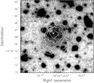
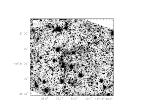
Due to the small field of view of the instrument () as compared to the expected size of the source, successive observations were taken following a raster pattern on the sky so as to cover the desired field. In order to reconstruct the full image of the sky covered by the observations a mosaicking procedure using the IDL programming language was developed. The procedure makes use of the IDL Astronomy User’s Library functions CORREL_IMAGES and CORRMAT_ANALYZE to determine relative shifts between subimages with 1 pixel accuracy. A sky level for each of the subexposures is first computed and subtracted using IDL DAOPHOT SKY procedure. (This has the consequence that any large-scale emission extending smoothly over most of the subexposure field of view would be subtracted out; any such large-scale synchrotron emission could however be detectable in polarisation with VLT/ISAAC, see Sect. 2.2.) Having determined the offsets, in the final step a mosaic (size of ) is created by stacking up and averaging the offset and sky corrected subimages. The top panel of Fig. 1 shows the final mosaicked image. The presented region is smaller than the size of the PWN in SNR G21.5-0.9 and covers the X-ray compact nebula region (e.g. Camilo et al., 2006).
Within a circular region of in diameter centred on the pulsar position, stars which have their brightness in the 2MASS K band (Skrutskie et al., 2006) determined were identified. Their fluxes, measured via aperture photometry, allowed for calculation of a photometric zero point between the instrumental system and the 2MASS K band. The photometric zero point was later used in the transformation of the measured flux to an apparent magnitude for the extended emission structure detected around the pulsar position.
2.2 VLT/ISAAC - polarimetry
Polarimetric observations of G21.5-0.9 were taken in the Ks filter with the ISAAC444http://www.eso.org/sci/facilities/ paranal/instruments/isaac/ instrument mounted on the ESO Very Large Telescope. The instrument uses a Wollaston prism, which splits the incoming radiation beam into two perpendicularly polarised beams, giving on one CCD plate two images of the same object separated by . In order to avoid sources overlapping, a special mask made of alternating opaque (width ) and transmitting stripes (width ) is inserted before the Wollaston prism. This instrumental set-up produces a CCD image containing altogether six subimages of the sky - three different stripes of the sky imaged at the same time in two perpendicular polarisations. Due to the non-standard mosaic reconstruction required, dedicated procedures performing the basic data reduction were developed. A sky flat field was obtained for each of the six stripes separately from median combination of all the images taken with the same angle (see below), each normalised to its median. A raster pattern was applied when performing the polarimetric imaging of G21.5-0.9 in order to obtain continuous coverage of a FOV containing the entire PWN. The complete image in any of the polarisation beams was then obtained using the mosaicking procedure described in Sect. 2.1, adapted to the specific character of the ISAAC polarimetric data, including sky level determination for each stripe in each image.
The polarimetric imaging was carried out with two different position angle settings of the instrument (measured North to East), namely with and , allowing for determination of a linear polarisation degree , which in terms of the Stokes parameters , and (see e.g. di Serego Alighieri, 1997, for the Stokes parameters definition) can be expressed as:
| (1) |
where:
| (2) |
and determination of a polarisation angle:
| (3) |
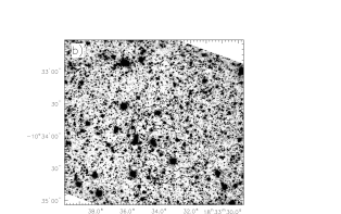
We note that the instrumental set-up is unable to measure any circular polarisation which might also be present. The derived polarisation angle (Eq. 3) is expressed in the detector reference frame. To refer it to the celestial reference frame a counter-rotation of with respect to the instrument position angle is applied following e.g. Eq. (9) of Landi Degl’Innocenti et al. (2007). In the celestial reference frame the polarisation angle is measured with respect to the North Celestial Meridian (North to East). The bottom panel of Fig. 1 shows the central part of G21.5-0.9, where the X-ray compact nebula is situated, as seen in the total intensity .
Polarisation standard stars were also observed and their linear polarisation degree and angle were measured in order to verify determination of polarisation parameters for the compact nebula region. The standard stars were chosen following the ISAAC list of polarised standard stars. We used R CrA15 and HD 188112. The measurements for R CrA15 in the Ks filter yield and determined North through East. The result is in fairly good agreement with the known polarisation for this object at shorter wavelengths - e.g., in the H band and and in the J band and (Whittet et al., 1992). For HD 188112 we get and .
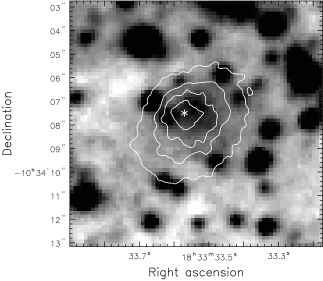
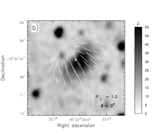
For the central region of G21.5-0.9 two maps, of linear polarisation fraction and linear polarisation intensity , were created. They are presented in Figure 2. For presentation purposes pixels with signal of below the sky value - as determined in the total intensity image - were masked in the map. In both maps an extended blob of polarised emission surrounding the PSR J1833-1034 position is visible. In order to show the behaviour of the polarisation angle across the nebula the electric field vectors are overlaid on the map. They were determined from the signal integrated over circular regions () spread across the polarised emission nebula. A gradual change in the polarisation angle is visible when moving from the SE to NW part of the torus region and its implications are discussed in more detail in Sect. 4.1.
Similarly as for the CFHT observations, the flux of the emission coincident with the putative pulsar wind torus identified in the averaged total intensity image was determined. To compute the photometric zero point, flux measurements for the polarimetric standards were used together with their 2MASS K magnitudes.
2.3 Spitzer
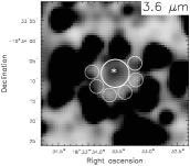
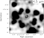
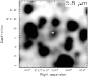
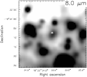
SNR G21.5-0.9 was observed with the Infrared Array Camera (IRAC) and Multiband Imaging Photometer (MIPS) onboard the Spitzer Space Telescope as part of observing programme ID 3647. Using the Spitzer Heritage Archive, post-Basic Calibrated Data (post-BCDs) containing mosaicked images of the G21.5-0.9 region were obtained for all IRAC bands and the 24 m MIPS band. The IRAC observations at 3.6, 4.5, 5.8 and 8.0 m were carried out on 15 September 2005, while the MIPS 24 m observation was taken on 11 April 2005. Figure 3 shows the central part of G21.5-0.9 in all IRAC bands.
 |
 |
 |
 |
2.4 VLT/ISAAC - [Fe II] imaging
G21.5-0.9 was also observed in the [Fe II] 1.64 m filter and in a neighbouring narrow-band 1.71 m filter with the ISAAC instrument (in standard imaging mode). A dark correction was applied to all frames following the standard approach using IDL procedures written to handle the ISAAC data. In each of the filters the successive exposures were performed in a wide raster pattern so as to cover the sky area where emission from the PWN, as well as a dense part of the SNR shell, could be expected. Large shifts between exposures were used to ensure that a given camera pixel fell outside any diffuse emission from G21.5-0.9 in most frames. A sky flat field for each of the narrow-band filters could then be constructed by median combination of all exposures taken on the same night (each scaled such that its median was unity). These sky flat fields were divided into the science frames following the standard approach. The IDL mosaicking procedure that also determines the sky level for each of the subexposures (see Sect. 2.1) was applied to obtain the final image in both the [Fe II] 1.64 m and 1.71 m filters.
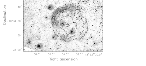
In order to minimise confusion from faint stars which is evident in the [Fe II] 1.64 m image (Fig. 4, panel a), we subtracted from it the 1.71 m image (Fig. 4, panel b). To compensate for the difference in stellar fluxes in different filters, an overall normalisation factor was computed from measured star fluxes in both narrow-band filters () assuming that star colour effects can be neglected over the small wavelength difference. A simple subtraction of the aligned and scaled 1.71 m image yields rather conspicuous stellar residua, however, due in large part to different PSFs in the two images owing to changing observing conditions. An improved subtraction was thus performed using a PSF equalisation procedure, which also ensured image alignment to sub-pixel accuracy, proceeding in the following way. We used 20 copies of the two original images with integer pixel offsets (all those with a total 2-D offset less than 2.5 pixels), and computed the linear combination of all these images, and a uniform background, which yielded minimal residua and a minimal contribution from the offset images. This optimisation was performed using a central image area which had negligible diffuse emission but a PSF as close as possible to the average one within the PWN area. The result is shown in panel c of Fig. 4: the effectiveness of the subtraction procedure, in the PWN area in particular, can be gauged by comparison with panel a, which shows the unsubtracted image in the same intensity scale. Some residua remain, including ”halos” around brighter stars, and may be due in part to non-linearities in instrument response, as well as to intrinsic differences in stellar spectra between the 1.64 m and 1.71 m bands.
Panel c of Figure 4 reveals, after the above subtraction, diffuse emission in the [Fe II] 1.64 m filter coincident with parts of the PWN in G21.5-0.9. Extended emission in the shape of a partial ring is clearly visible. Chandra ACIS contours are overlaid to show the PWN extent in X-rays. The surface brightness for the NE and S rims of the [Fe II] 1.64 m emission was computed. The flux calibration was performed using stars that have 2MASS H magnitudes determined and that could be identified in the observed field. Detailed discussion of the results can be found in Sect. 3.3.
3 Results
3.1 Compact Core – near-infrared
The field of view (FOV) of the central part of the AOB-KIR mosaicked image with the best S/N is approximately . It covers the central part of the PWN as identified by X-ray observations, and in particular the compact nebula around the pulsar (Slane et al., 2000). The observed field is rich in stars which can confuse any NIR emission coming from G21.5-0.9. Using a brightness scale in which stars are saturated, a clearly extended region of emission (compared to the instrument’s ) emerges from the background (Fig. 1, top panel). Its size of in diameter is comparable with the size of the X-ray compact nebula. Its apparent centre is slightly shifted towards the SW with respect to the pulsar position and (Camilo et al., 2006), but more extended emission may be confused with the stars that are situated to the NE of the pulsar. It is worth noting that the X-ray morphology of the emission region around the pulsar position (Camilo et al., 2006; Matheson & Safi-Harb, 2010) is similar to the one seen in the present near-infrared data, and can be caused by a Doppler-boosted toroidal structure surrounding the pulsar.
To extract the flux from the extended emission nebula a circular aperture in diameter around the pulsar position was used. The contributions to the flux of the nebula from stars located within a radius of the pulsar were subtracted by performing aperture photometry. The measured flux for the compact nebula corrected for interstellar extinction is mJy. The existence of this emission blob is confirmed by the polarimetric observations. No other significant diffuse emission is detected.
Each of the mosaicked images, i(0), i(45), i(90) and i(135), obtained from the subimages taken in the polarimetric mode of the ISAAC instrument, has a FOV of . In all cases it includes the entire region where the X-ray PWN is identified. The detected diffuse emission, which can be seen in the total intensity image (Fig. 1, bottom panel), is restricted only to the very central region of the PWN. It is slightly extended and compatible in size and position with the emission blob detected with AOB-KIR in the K’ filter.
Measurements of the degree of linear polarisation and the polarisation angle reveal highly polarised emission from the nebula with a regular structure of the electric field (Fig. 2, panel b). As can be seen from the map (Fig. 2, panel a) this polarised emission extends within the X-ray compact nebula and is only important where the star contamination is minimal. To the NE of the pulsar position, but still within the X-ray compact nebula, a region where the linear polarisation degree is smaller than 0.1 can be identified (Fig. 2, panel a). As seen from the total intensity image (Fig. 1, bottom panel), this is also the region where strong stellar contamination is present. The linear polarisation fraction averaged over the emission region is high, ; moreover, in some regions within the polarisation nebula is even as high as . The high degree of linear polarisation points to the synchrotron nature of the observed radiation and a highly ordered magnetic field structure.
As mentioned before, the measurements of across the compact nebula reveal a regular structure of the radiation electric field which is illustrated as white vectors in the b panel of Fig. 2. In the central part of the nebula the electric field vectors are oriented in the NE-SW direction. In the outer regions of the nebula, vectors tend to bend away from the NE-SW direction in a twofold way: moving to the NW vectors rotate anticlockwise; in the SE part vectors rotate clockwise with respect to the electric field direction determined in the central part of the polarisation nebula. The change in orientation of the electric field vectors is accompanied by a steady decrease in the linear polarisation fraction .
A circular aperture similar in size to that used for the CFHT flux measurements was used to extract the counts from the detected polarised emission blob. Star contamination to the measured flux was reduced by their standard photometry measurements. The dereddened flux for the emission blob derived from the averaged total intensity is mJy; although it is compatible within uncertainties, we consider this value less reliable than the one obtained from the AOB-KIR observations (see Sect. 4.2).
 |
 |
 |
|
3.2 Compact Core – mid-infrared
No large-scale extended emission associated with the PWN is seen in IRAC bands. However, in the PWN centre a compact emission blob is present (Fig. 3). It is clearly visible in all IRAC bands and its extent is comparable with the size of the putative pulsar wind torus seen in X-rays (Camilo et al., 2006) and in the near-infrared. For the IRAC observations the source flux was obtained using an extraction region with a radius of (large circle in the top left panel of Fig. 3). To estimate the background level, circular regions with a radius (small circles in the top left panel of Fig. 3) were chosen in the vicinity of the source extraction region. The average value from these regions was taken to represent the background level at the source position. Because the aperture used for the flux estimation in the IRAC bands was different from the aperture used for the Spitzer calibration stars an aperture correction, as described in IRAC Handbook555http://ssc.spitzer.caltech.edu/irac/iracinstrumenthandbook/, was applied to the computed fluxes. In order to estimate the compact nebula’s flux at MIPS 24 m standard aperture photometry was used. A source extraction region with radius of was used. The background was estimated using an annulus with an inner radius of and an outer radius of . To obtain the final value of the measured flux an aperture correction was applied as described in the MIPS Handbook666http://ssc.spitzer.caltech.edu/mips/mipsinstrumenthandbook/. Spitzer IRAC and MIPS 24 m fluxes are presented in Table 2. The flux uncertainties reflect the variations in the background level between different background regions, as well as the uncertainty in the extinction correction for the de-reddened fluxes.
| Instrument | Observed Flux | De-reddened Flux | |
|---|---|---|---|
| [m] | [mJy] | [mJy] | |
| IRAC | |||
| 3.6 | 0.53 0.19 | 0.94 0.45 | |
| 4.5 | 0.74 0.14 | 1.19 0.49 | |
| 5.8 | 0.88 0.20 | 1.34 0.49 | |
| 8.0 | 0.89 0.22 | 1.38 0.71 | |
| MIPS | |||
| 24.0 | 2.47 0.67 | 4.37 2.13 |
3.3 Pulsar Wind Nebula
The mosaicked image taken in the [Fe II] 1.64 m and 1.71 m filters (see Sect. 2.4) covers a FOV of . This includes both the PWN region and the North Spur region (a bright spot located in the northern part of the X-ray halo surrounding the PWN (Bocchino et al., 2005)). By subtracting the 1.71 m image (corrected for the PSF and average star flux difference between the filters) from the [Fe II] 1.64 m image (see Sect. 2.4) we minimise the stellar contamination to any [Fe II] 1.64 m line emission that can be present in the observed region. The resultant image is presented in panel c of Fig. 4. No [Fe II] line emission associated with the North Spur is detected. There is, however, extended ( in diameter) [Fe II] emission associated with the PWN. Its shape follows the outer contours of the X-ray nebula (Fig. 4, panel b). The brightness distribution is non-uniform; a partial ring-like structure has a maximum of emission in the NE part. Going towards the SW, the emission fades leaving only a few faint patches of [Fe II] emission which fall within the X-ray contours of the PWN (Fig. 4, panel c). The brightest NE portion of the ring shows clear limb-brightening with a well-defined outer edge. To the SW from the pulsar position an emission blob, probably an artefact associated with the bright star (as seen next to other bright stars in the FOV) rather than with the PWN material, is apparent. The mean surface brightness of the NE part of [Fe II] line emission is erg s-1 cm-2 arcsec-2 while for the southern rim it is erg s-1 cm-2 arcsec-2.
4 Interpretation
Both the emission detected with AOB-KIR, Spitzer and the ISAAC polarimetric observations and also the structure seen in the [Fe II] 1.64 m emission line, can be interpreted within a composite supernova remnant evolutionary scheme (e.g. Gaensler & Slane, 2006; van der Swaluw et al., 2001; Reynolds & Chevalier, 1984). According to this evolutionary scheme a supernova (SN) explosion drives a blast wave into the surrounding interstellar medium (ISM). At the same time in the interior of the expanding SNR a pulsar wind nebula evolves. It is powered by the newly born pulsar through its relativistic magneto-hydrodynamic wind. At early times, the pulsar energy input causes the PWN’s expansion to accelerate, driving a shock into the inner edge of the uniformly expanding ejecta. Inside the PWN, at the point where the pulsar wind ram pressure is equilibrated by the pressure exerted by the surrounding medium, a pulsar wind termination shock (WTS) is formed. The schematic structure of such a young composite SNR is presented in Figure 5.

4.1 Polarisation - Wind Termination Shock
The high degree of linear polarisation measured across the emission blob seen in the Ks band (see Sect. 3.1) points to its synchrotron origin. Simultaneously, the orientation of the electric field vectors (Fig. 2, bottom panel) suggests that the region where synchrotron radiation is produced has a toroidal magnetic field. Such conditions are expected to be found in the wind termination shock region (Fig. 5). The relativistic particles flowing upstream of the shock do not radiate. Only after being accelerated at the shock, can they produce synchrotron radiation in the downstream flow. The best example in support of such a scenario is the torus in the Crab Nebula (Hester, 2008, and references therein). When viewed in polarised light it shows magnetic field structure that is aligned along wisps and fibrous structures which are present in the torus, and which follow its shape. For some of the wisps a high degree of linear polarisation, near 0.7, is measured.
Recent MHD simulations studying optical polarisation in the inner parts of pulsar wind nebulae (Bucciantini et al., 2005; Del Zanna et al., 2006; Volpi et al., 2009) predict that emission from a wind termination shock region should be highly polarised. In these simulations a pure toroidal structure of magnetic field and a radial flow of particles are assumed. The maximum value of linear polarisation fraction, close to 70%, is expected from the WTS region close to the torus symmetry axis as projected on the sky. When moving away from the axis, the polarisation progressively decreases to values smaller than 50%. In addition, close to the torus edges, regions that are almost completely depolarised can be found (see Fig. 2 of Bucciantini et al., 2005). Simulations also show that the polarisation angle should change across the emitting region. In the parts close to the symmetry axis of the torus, the electric vector should be aligned with the axis and its inclination with respect to the axis should increase while moving away from it. The region where the electric vector becomes perpendicular to the symmetry axis depends on the inclination angle of the torus with respect to the sky, and also on the bulk flow speed. Concerning the latter dependence, the position where the polarisation vector becomes perpendicular to the axis moves closer towards the axis with increasing value of the bulk speed (Bucciantini et al., 2005).
Similar behaviour to that predicted by MHD simulations is found in our polarisation observations of the central part of G21.5-0.9 (see Sect. 3.1), which supports the claim that in the region of the wind termination shock a toroidal magnetic field is present. From the investigation of the observed polarisation angle swing, the probable orientation of the symmetry axis of the toroidal field as projected on the sky is (measured North to East). In this scenario, is also the position angle of the pulsar spin axis as projected on the sky, which is in agreement to the value proposed by Camilo et al. (2006). The nebula seen in the Ks band can be described as an ellipse with semimajor axis of and semiminor axis of . The ellipse minor axis is oriented at , so it is parallel to the toroidal magnetic field symmetry axis as projected on the sky. However, due to the Doppler boosting experienced by the relativistic particles escaping the wind termination shock, the visible size of the emission region cannot be simply translated into the shock radius. A vital part of the WTS may be invisible because the size of the emitting region highly depends on the bulk flow speed in the WTS region (Bucciantini et al., 2005). If the emitting torus is not seen edge-on, but is inclined with respect to the plane of the sky, the Doppler boosting effect could possibly explain the shift of the compact nebula emission towards SW with respect to the pulsar position. To more accurately estimate the orientation of the toroidal magnetic field and the flow speed, detailed modelling is needed. However, by simple comparison with the numerical results of Bucciantini et al. (2005), Del Zanna et al. (2006) and Volpi et al. (2009) one may expect that the particle flow speed in the WTS region is high ().
4.2 Nonthermal Emission Spectrum
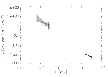
Figure 6 presents the spectral energy distribution of the compact nebula based on our flux measurements in the CFHT/AOB-KIR, Spitzer IRAC 3.6, 4.5, 5.6, 8.0 m and MIPS 24 m bands, and its intrinsic X-ray spectrum obtained from Chandra observations presented by Camilo et al. (2006). The plotted IR fluxes are the values corrected for the interstellar extinction using the local ISM table of Chiar & Tielens (2006), where was estimated from following Gorenstein (1975) and Cardelli et al. (1989). A simple power law , where is the spectral index, was fitted to the infrared fluxes using a least-squares fitting method that takes into account the uncertainties of the measured fluxes as their weights. In the fit the flux value obtained from the VLT/ISAAC-POL averaged total intensity was not included because the flux value from CFHT/AOB-KIR observations is a more accurate representation of the compact nebula flux at m. This is because the higher resolution (smaller PSF) of CFHT/AOB-KIR allows for much more accurate stellar subtraction in the crowded compact nebula field, which is difficult in the case of VLT/ISAAC-POL and in turn leads to an overestimation of the measured flux. The fitting to the rest of the IR fluxes yields the spectral index . The obtained power law with its uncertainty is presented in Fig. 6 as the light grey bow tie region.
The X-ray spectrum in the keV energy range was obtained from Chandra ACIS observations (Camilo et al., 2006) using a circular extraction region with radius around the PSR. The background level was estimated using an annulus with radius . Using the best-fit value of cm-2 for the entire nebula (Slane et al., 2000) this yields a photon index of and unabsorbed flux in the keV energy range erg s-1 cm-2. Allowing the column density to be determined just from the fit of the compact region yields similar values of cm-2, and erg s-1 cm-2. Comparison of the fitted IR spectrum with the X-rays (Fig. 6) suggests that the spectrum must flatten between infrared and X-rays. Given the unusual implications of such a result on the underlying particle spectrum, it is important to consider possible factors that could complicate the interpretation of the X-ray spectrum. There are two primary sources of potential bias: contamination from the central pulsar, and dust scattering effects.
Regarding the pulsar contamination, to estimate a point source contribution to the unabsorbed flux of the compact nebula, Camilo et al. (2006) use Chandra HRC data to model the spatial emission around PSR J1833-1034 as a point source and a 2-D Gaussian. Converting their best-fit count rate of the point-like component into a flux using cm-2 and an assumed photon index of 1.5 yields an unabsorbed flux erg s-1 cm-2 (about 2% of the unabsorbed flux obtained for the compact nebula). This contribution is insufficient to account for the apparent difference in spectral index between the X-ray and IR bands (and the reduced flux upon subtracting the point source contribution marginally increases the difficulty in matching the spectra).
The properties of X-ray scattering from dust grains are well known (see e.g. Smith & Dwek, 1998), but modelling of X-ray halos of diffuse sources is a difficult task, because the effect is non-local. Bocchino et al. (2005) have modelled the X-ray halo detected around G21.5-0.9, showing that it is mostly an effect of dust scattering, deriving halo parameters, like the scattering optical depth : from this energy dependence it is apparent that lower-energy photons are scattered with much higher efficiency. An additional effect of scattering is a radial dependence of the best-fit column density (), which in G21.5-0.9 ranges from cm-2 in the outskirts of the PWN, up to cm-2 in the very central regions (see Fig. 3 in Bocchino et al., 2005).
A consequence of scattering is a deficiency of soft photons in the central regions, which leads standard spectral analysis routines to overestimate the absorption column density; conversely, the surrounding regions receive the scattered photons and show an excess of soft photons that leads to a negative bias on the estimated . Since in principle similar biases could affect the estimates of the spectral index and unabsorbed flux, depending on the details of the data analysis, we set upper limits to those possible biases. We have chosen the energy range keV for our fits to the spectrum of the inner torus: this is a good compromise for weighting harder photons (only weakly affected by scattering) but still retaining good statistics. With this energy cut we cannot independently determine the value of , but instead consider a range of parameters, chosen from 2.0 to cm-2 ( cm-2 being the average value obtained from a fit to the whole PWN).
Another question is whether or not to use as background the emission of the surrounding PWN: the emission in the surroundings of the torus is partly contaminated by the halo of the torus itself, and some of the photons emitted by the outer PWN are scattered into the area on which the torus extends. In Table 3 we present the results for the grid of cases mentioned above. From this we can conclude that conservative error intervals on the parameters, taking also into account dust scattering effects, are the compact nebula photon index of and the unabsorbed flux of erg s-1 cm-2.
| NH | ||
|---|---|---|
| [ cm-2] | [ erg s-1 cm-2] | |
| Background from surrounding annulus | ||
| 2.0 | 1.43 | 7.7 |
| 2.2 | 1.47 | 7.6 |
| 2.4 | 1.51 | 7.7 |
| No background | ||
| 2.0 | 1.49 | 9.6 |
| 2.2 | 1.53 | 9.7 |
| 2.4 | 1.57 | 9.7 |
We note that a joint fit between the X-ray and IR data, leaving all parameters free, yields cm-2 and . Applying these values to the X-ray data alone provides a good fit (), though the X-ray fit obtained with and as free parameters is statistically much better (). The results are similar when a dust-scattering component is included in the fitting process. While the spectral modeling thus argues for a spectral flattening between the IR and X-ray bands, it is clearly important to search for examples of such behavior in other sources given that the results here rely exclusively on somewhat modest differences in parameters from spectral fitting.
Even though the torus in G21.5-0.9 is not detected in the radio, it would appear that a further break or steepening must exist between the radio and IR bands. Using the radio map at 5 GHz (Bietenholz & Bartel, 2008) we can estimate an upper limit mJy to the radio flux of the compact nebula by integrating the signal within a radius of around the pulsar position. This can be compared to the 5 GHz flux Jy which one gets by extrapolating the fitted IR spectrum to the radio band. This extrapolated value is much higher than the estimated upper limit , which argues in favour of the existence of spectral break between the radio and IR bands. This would be expected because the radio spectrum of the torus presumably has the same index as the entire PWN (whose radio index is flatter than what has been measured here for the torus in the IR), because the particles responsible for the radio emission will not have suffered significant radiative losses in filling the nebula. Similar spectral behaviour is also observed for the torus in 3C 58 (Slane et al., 2008). These two cases show that the injection spectrum is complex, and not a pure power law. Fleishman & Bietenholz (2007) have calculated synchrotron spectra of a power-law distribution of electrons radiating in magnetic turbulence of prescribed properties. For appropriate choices of parameters, it is possible to produce a spectrum that could continue to steepen from radio to X-ray energies, as our data imply; however, the suggestion in our data of a flattening of the spectrum between IR and X-rays cannot be produced by such a model. Moreover, the Fleishman & Bietenholz (2007) calculations were applied to the integrated spectra of the PWNe and as such they may not be applicable to explain the spectra produced in the vicinity of the wind termination shock, which is the case for the spectrum presented in Fig. 6.
4.3 [Fe II] filaments - PWN shock
Studies carried out in the past 20 years on infrared emission from shell supernova remnants show that [Fe II] emission seen in shell SNRs is either induced by the reverse shock propagating back through the fast moving ejecta or produced at the forward shock from iron present in the circumstellar and/or interstellar medium. In the case of pulsar wind nebulae, by contrast, iron emission, if collisionally excited, is produced by the rapidly expanding PWN encountering the slow-moving cold ejecta (Fig. 5). This interpretation has been applied to observed [Fe II] lines at 17.9 and 26 m from G54.1+0.3 (Temim et al., 2010) and B0540-69.3 (Williams et al., 2008). Our imaging observations demonstrate that in SNR G21.5-0.9, the iron emission does in fact originate at the location of the PWN-ejecta interaction. The nature of this emission then characterizes the otherwise unobservable innermost supernova ejecta, material formed just above the mass cut within which material fell back to become the neutron star.
In G21.5-0.9 the detected [Fe II] 1.64 m emission - having a ring-like structure that is significantly brighter in the NE - follows the outer edge of the PWN (Fig. 4). This behaviour suggests that the [Fe II] emission is caused by the PWN driven shock that compresses the surrounding cold supernova ejecta (Fig. 5). Collisional excitation would then take place in the medium just behind the shock front. The low excitation energy means that only low shock velocities are required, perhaps as a result of shocks being driven into dense clumps in the ejecta, but it is also possible that the PWN forward-shock speed is slow due to its expansion into moving ejecta. Figuring out which one is more plausible in the case of G21.5-0.9 would require a dynamical model and/or spectroscopic study in search of density diagnostics in the line-emitting regions. The observed brightness difference between regions in the NE and SW could result from a density difference in the medium that the expanding PWN bubble encounters, which in turn would imply a difference in the PWN shock velocity in the NE part with respect to the SW.
A good example of the PWN expanding into a medium of nonuniform density is the Crab Nebula. Such conclusion is drawn based on observations of [O III] and [Ne V] emission, excited by the PWN shock, which forms so-called skin at the boundary of the Crab Nebula. The skin is visible around most of the outer edge of the nebula with the exception of its NW part (Sankrit & Hester, 1997). The lack of [O III] and [Ne V] emission is explained as due to variations in the density of the ejecta into which the nebula is expanding. This view is also supported by the morphology of Rayleigh-Taylor fingers (Loll et al., 2007), which shows SE-NW asymmetry. In the NW part of the Crab Nebula there are fewer fingers comparing to the SE. This asymmetry results from a preshock ejecta density lower in the NW than in the SE (Hester, 2008, and references therein).
However, another possible scenario may explain the [Fe II] 1.64 m line emission in PWNe. Graham et al. (1989) showed that the near-infrared iron emission detected in the Crab Nebula originates from optically thick filaments which are photoionized by the UV–X-ray component of the synchrotron continuum present in the PWN. In the general ISM, a measured line ratio ([Fe II] 1.64 m)/(Br) 1 is interpreted as the case of shock excitation, as radiative shocks destroy grains and return Fe to the gaseous state. In SNR ejecta, however, we do not know what fraction of Fe might be in grains initially, or what the Fe/H abundance ratio is, making this test inappropriate. In addition, as pointed out by Graham et al. (1989), in the Crab Nebula conditions leading to high values of ([Fe II] 1.64 m)/(Br) can also be found in the photoionized filaments. Thus, determining this line ratio as the sole factor discriminating between the two scenarios may not be conclusive. Recent studies of SNRs where [Fe II] 1.64 m is detected, e.g. G11.2-0.3 (Koo et al., 2007) and 3C 396 (Lee et al., 2009), show that iron emission can be explained by a radiative shock propagating into the gas with a velocity km s-1. The iron line-emitting regions are characterised by high electron densities cm-3 and electron temperatures of order a few times 103 K. This can be contrasted with the conditions found for the photoionized case in the Crab Nebula where cm-3 and K (Graham et al., 1989). Thus in order to try to discriminate between the two scenarios in the case of G21.5-0.9, spectroscopic observations of the [Fe II] line-emitting regions are needed.
5 Conclusions
In this paper we report the first detection in the infrared band of emission emanating from the compact nebula region in SNR G21.5-0.9 (2 radius around the pulsar position) through imaging and polarimetry. The toroidal structure of the magnetic field in the compact nebula is inferred from polarimetric observations in the Ks band. The high degree of linear polarisation together with the observed swing of the electric field vector across the nebula confirms that the observed radiation is synchrotron emission from relativistic particles accelerated at the wind termination shock and radiating in the downstream flow. The infrared spectrum of the compact nebula can be described as a power law with spectral index ; when combined with X-ray results from Chandra observations (Camilo et al., 2006), it suggests that the spectrum flattens between the infrared and X-ray bands.
The detection of [Fe II] 1.64 m emitting material within the PWN of G21.5-0.9 is also reported. This iron emission is detected in the NE and in the SW of the PWN. The determined surface brightness of the SW emission is weaker compared to that of the NE region. It is important to point out that the detected [Fe II] emission has the shape of a limb-brightened broken ring (40 radius), which follows the edge of the X-ray and radio PWN, but is concentrated inside the PWN boundary. Most probably the observed iron emission originates from cold supernova ejecta shocked by the expanding PWN bubble. In this case collisionally excited iron radiates in the medium behind the shock. However, to confidently discriminate between the case of shock excitation and photoionization by the synchrotron continuum, spectroscopic observations of the iron line-emitting material are needed. Line profiles can give shock velocities, while observation of additional spectral lines can provide density and temperature diagnostics to constrain shock models. Important information to be gained this way can include the speed of shocks causing excitation and ionization; the expansion rate of the PWN; abundances of the shocked material; and possible contributions of dust to the IR continuum, allowing inferences on newly synthesized dust. G21.5-0.9 thus joins the small elite class of objects, along with G54.1+0.3 and B0540-69.3, where IR observations of PWN interactions are illuminating the deep interior of a core-collapse supernova.
The present work demonstrates that infrared observations, both imaging and polarimetry, are an effective tool for detecting optically obscured pulsar wind nebulae and for studying their inner structure.
Acknowledgements.
This research is based in part on observations obtained at the Canada-France-Hawaii Telescope (CFHT) which is operated by the National Research Council of Canada, the Institut National des Sciences de l’Univers of the Centre National de la Recherche Scientifique of France, and the University of Hawaii. It is also based on observations made with ESO Telescopes at the La Silla Paranal Observatory under programme ID 69.D-0279(A, B). This work is based in part on observations made with the Spitzer Space Telescope, which is operated by the Jet Propulsion Laboratory, California Institute of Technology under a contract with NASA. This publication makes use of data products from the Two Micron All Sky Survey, which is a joint project of the University of Massachusetts and the Infrared Processing and Analysis Center/California Institute of Technology, funded by the National Aeronautics and Space Administration and the National Science Foundation. We thank M. F. Bietenholz for providing the radio map of G21.5-0.9 in numerical form, and an anonymous referee for comments which substantially improved the clarity of the paper. This research was partially supported by MNiSW grant N203 387737 and ECO-NET grant 18874 WA. This work was carried out within the framework of the European Associated Laboratory ”Astrophysics Poland-France”. A. Zajczyk acknowledges partial support from the Scholarship for PhD students ”Stypendium dla doktorantów 2008/2009 - ZPORR”. P. Slane acknowledges partial support from NASA contract NAS8-03060 and Spitzer grant JPL 1265776.References
- Asaoka & Koyama (1990) Asaoka, I. & Koyama, K. 1990, PASJ, 42, 625
- Becker & Szymkowiak (1981) Becker, R. H. & Szymkowiak, A. E. 1981, ApJ, 248, L23
- Bietenholz & Bartel (2008) Bietenholz, M. F. & Bartel, N. 2008, MNRAS, 386, 1411
- Bocchino et al. (2005) Bocchino, F., van der Swaluw, E., Chevalier, R., & Bandiera, R. 2005, A&A, 442, 539
- Bucciantini et al. (2005) Bucciantini, N., Del Zanna, L., Amato, E., & Volpi, D. 2005, A&A, 443, 519
- Camilo et al. (2006) Camilo, F., Ransom, S. M., Gaensler, B. M., et al. 2006, ApJ, 637, 456
- Cardelli et al. (1989) Cardelli, J. A., Clayton, G. C., & Mathis, J. S. 1989, ApJ, 345, 245
- Chiar & Tielens (2006) Chiar, J. E. & Tielens, A. G. G. M. 2006, ApJ, 637, 774
- Davelaar et al. (1986) Davelaar, J., Smith, A., & Becker, R. H. 1986, ApJ, 300, L59
- Del Zanna et al. (2006) Del Zanna, L., Volpi, D., Amato, E., & Bucciantini, N. 2006, A&A, 453, 621
- di Serego Alighieri (1997) di Serego Alighieri, S. 1997, Instrumentations for large telescopes, 000, 287
- Fleishman & Bietenholz (2007) Fleishman, G. D. & Bietenholz, M. F. 2007, MNRAS, 376, 625
- Fürst et al. (1988) Fürst, E., Handa, T., Morita, K., et al. 1988, PASJ, 40, 347
- Gaensler & Slane (2006) Gaensler, B. M. & Slane, P. O. 2006, ARA&A, 44, 17
- Gallant & Tuffs (1999) Gallant, Y. A. & Tuffs, R. J. 1999, ESASP, 427, 313
- Gorenstein (1975) Gorenstein, P. 1975, ApJ, 198, 95
- Graham et al. (1989) Graham, J. R., Wright, G. S., & Longmore, A. J. 1989, in ESA Special Publication, Vol. 290, Infrared Spectroscopy in Astronomy, ed. E. Böhm-Vitense, 169–175
- Gupta et al. (2005) Gupta, Y., Mitra, D., Green, D. A., & Acharyya, A. 2005, Current Science, 89, 853
- Hester (2008) Hester, J. J. 2008, ARA&A, 46, 127
- Kennel & Coroniti (1984) Kennel, C. F. & Coroniti, F. V. 1984, ApJ, 283, 694
- Koo et al. (2007) Koo, B., Moon, D., Lee, H., Lee, J., & Matthews, K. 2007, ApJ, 657, 308
- Landi Degl’Innocenti et al. (2007) Landi Degl’Innocenti, E., Bagnulo, S., & Fossati, L. 2007, ASP Conference Series, 364, 495
- Lee et al. (2009) Lee, H., Moon, D., Koo, B., Lee, J., & Matthews, K. 2009, ApJ, 691, 1042
- Loll et al. (2007) Loll, A. M., Hester, J. J., Blair, W. P., & Sankrit, R. 2007, Bull.Am.Astron.Soc., 38, 916
- Matheson & Safi-Harb (2010) Matheson, H. & Safi-Harb, S. 2010, ApJ, 724, 572
- Oliva et al. (1989) Oliva, E., Moorwood, A. F. M., & Danziger, I. J. 1989, A&A, 214, 307
- Reynolds & Chevalier (1984) Reynolds, S. P. & Chevalier, R. A. 1984, ApJ, 278, 630
- Safi-Harb et al. (2001) Safi-Harb, S., Harrus, I. M., Petre, R., et al. 2001, ApJ, 561, 308
- Salter et al. (1989) Salter, C. J., Reynolds, S. P., Hogg, D. E., Payne, J. M., & Rhodes, P. J. 1989, ApJ, 338, 171
- Sankrit & Hester (1997) Sankrit, R. & Hester, J. J. 1997, ApJ, 491, 796
- Skrutskie et al. (2006) Skrutskie, M. F., Cutri, R. M., Stiening, R., et al. 2006, AJ, 131, 1163
- Slane et al. (2000) Slane, P., Chen, Y., Schulz, N. S., et al. 2000, ApJ, 533, L29
- Slane et al. (2008) Slane, P., Helfand, D. J., Reynolds, S. P., et al. 2008, ApJ, 676, L33
- Smith & Dwek (1998) Smith, R. K. & Dwek, E. 1998, ApJ, 503, 831
- Temim et al. (2006) Temim, T., Gehrz, R. D., Woodward, C. E., et al. 2006, AJ, 132, 1610
- Temim et al. (2010) Temim, T., Slane, P., Reynolds, S. P., Raymond, J. C., & Borkowski, K. J. 2010, ApJ, 710, 309
- Tian & Leahy (2008) Tian, W. W. & Leahy, D. A. 2008, MNRAS, 391, L54
- Truelove & McKee (1999) Truelove, J. K. & McKee, C. F. 1999, ApJS, 120, 299
- van der Swaluw et al. (2001) van der Swaluw, E., Achterberg, A., Gallant, Y. A., & Tóth, G. 2001, A&A, 380, 309
- Volpi et al. (2009) Volpi, D., Del Zanna, L., Amato, E., & Bucciantini, N. 2009, ArXiv e-prints, 0903.4120
- Whittet et al. (1992) Whittet, D. C. B., Martin, P. G., Hough, J. H., et al. 1992, ApJ, 386, 562
- Williams et al. (2008) Williams, B. J., Borkowski, K. J., Reynolds, S. P., et al. 2008, ApJ, 687, 1054