Interelectronic-interaction effects on the two-photon decay rates of heavy He-like ions

Abstract

Based on a rigorous QED approach a theoretical analysis is performed for the two-photon transitions in heavy He-like ions. Special attention is paid to the interelectronic-interaction corrections to the decay rates that are taken into account within the two-time Green-function method. Detailed calculations are carried out for the two-photon transitions $2^{1}S_{0}\rightarrow 1^{1}S_{0}$ and $2^{3}S_{1}\rightarrow 1^{1}S_{0}$ in He-like ions within the range of nuclear numbers $Z=28-92$. The total decay rates together with the spectral distributions are given. The obtained results are compared with experimental values and previous calculations.

I Introduction

The two-photon process involving simultaneous emission of two photons was theoretically predicted by Göppert-Mayer in 1931 Göppert-Mayer (1931). It arises from a second-order interaction between an atom and the electromagnetic field resulting in sharing the transition energy between the two photons. The energy distribution of the two-photon spontaneous emission forms a continuous spectrum in contrast to the one-photon process, where the photon frequency equals to the transition energy. Various characteristics of the two-photon transitions, such as total and energy-differential decay rates, angular and polarization correlations of the emitted photons were widely investigated for heavy hydrogenlike ions (see, e.g., Refs. Drake (1986); Santos et al. (1998); Surzhykov et al. (2005); Labzowsky et al. (2005); Amaro et al. (2009)). Due to the recent advances in the experimental technique heavy He-like ions became promising candidates for studying the two-photon decays in the high-$Z$ domain. Here the $2^{1}S_{0}$ state is of special interest, since this state primarily decays into the ground state via two-photon emission. The first theoretical two-photon decay rate of the $2^{1}S_{0}$ state in helium was presented by Dalgarno Dalgarno (1966). Later accurate nonrelativistic calculations, including the estimation of the relativistic effects, of the two-photon transition rates $2^{1}S_{0}\rightarrow 1^{1}S_{0}+2\gamma(\rm E1)$ for He-like ions were performed by Drake Drake (1986). The two-photon decay $2^{3}S_{1}\rightarrow 1^{1}S_{0}+2\gamma(\rm E1)$ was investigated theoretically as well Bely and Faucher (1969); Drake et al. (1969), although its rates are smaller than the corresponding one-photon M1 rates by a factor of about $10^{-4}$. Up to date the most accurate fully relativistic calculations of the two-photon decay rates of the $2^{1}S_{0}$ and $2^{3}S_{1}$ states in the highly charged ions were performed using relativistic configuration-interaction wave functions in Ref. Derevianko and Johnson (1997). Apart from the total and energy-differential decay rates the angular correlations in the two-photon decay of He-like ions have also been investigated recently Surzhykov et al. (2010).

The lifetimes of metastable $2^{1}S_{0}$ level in He-like ions have been measured up to $Z=41$. The most precise measurements have been made in Kr³⁴⁺ Marrus et al. (1986), Br³³⁺ Dunford et al. (1993a), and Ni²⁶⁺ Dunford et al. (1993b) where uncertainties of about 1% have been reported. However, till present the two-photon decay of the $2^{3}S_{1}$ level in He-like ions has not been observed. As opposed to the total decay rate measurements, the observation of the energy-differential spectrum carries more detailed information about the entire atomic structure. Several experimental efforts have been made during the last two decades to accurately determine the spectral shape of the two-photon distribution for $2^{1}S_{0}$ decay in He-like ions Mokler et al. (1990); Ali et al. (1997); Schäffer et al. (1999). The cleanest spectrum has been obtained recently in Refs. Kumar et al. (2009); Trotsenko et al. (2010), unambiguously confirmed predictions of relativistic many-body theory as compared to the nonrelativistic calculations.

Since the two electrons in He-like ions are strongly correlated, it is important to take into account the interelectronic-interaction effects when studying the two-photon decays. In previous calculations the correlation effects were accounted for by means of nonrelativistic Hylleraas variational wave functions Drake (1986), relativistic configuration-interaction (CI) wave functions Derevianko and Johnson (1997), or by means of relativistic wave functions in screening potentials Savukov and Johnson (2002); Trotsenko et al. (2010); Surzhykov et al. (2010); Shabaev et al. (2010). However, a rigorous description of high-$Z$ systems requires the quantum electrodynamic (QED) approach, which treats systematically radiative and correlation corrections order by order. Future progress in the experimental techniques will allow to observe QED corrections to the transition amplitudes. In particular, recent precise measurements of the one-photon decay rates of the $(1s^{2}2s^{2}2p)\,^{2}P_{3/2}$ state in B-like Ar Lapierre et al. (2005, 2006) have been shown to be sensitive to the one- and many-electron QED effects Tupitsyn et al. (2005); Volotka et al. (2006); Volotka et al. (2008a). The QED treatment of the correlation effects differs from the many-body perturbation theory by the frequency-dependent contribution. The first QED evaluation of the interelectronic-interaction correction of first order in $1/Z$ to the one-photon decay rates was performed in Ref. Indelicato et al. (2004) employing the two-time Green-function method V. M. Shabaev, Izv. Vuz. Fiz. 33, 43 [Sov. Phys. J. 33, 660 (1990)].() (1990); V. M. Shabaev, Teor. Mat. Fiz. 82, 83 [Theor. Math. Phys. 82, 57 (1990)].() (1990); Shabaev (2002); later these calculations were confirmed in Ref. O. Yu. Andreev et al. (2009) by means of the line profile approach O. Yu. Andreev et al. (2008). The main goals of the present paper are the derivation of formulas for the interelectronic-interaction corrections to the two-photon decays from the first principles of QED and the numerical evaluations of the two-photon transitions $2^{1}S_{0}\rightarrow 1^{1}S_{0}$ and $2^{3}S_{1}\rightarrow 1^{1}S_{0}$ in the He-like ions. The paper is organized as follows: In the next section the process of the two-photon emission is described in the framework of the two-time Green-function method. The calculation formulas for the first-order interelectronic-interaction corrections to the two-photon transition amplitude are derived starting in the zeroth-order approximation with the Coulomb potential of the nucleus and with a local screening potential. In Sec. III we present the numerical results for the two-photon decay rates of $2^{1}S_{0}$ and $2^{3}S_{1}$ states in He-like ions. Beyond the dominant channel of the emission of two electric-dipole (E1) photons the higher multipoles contributions are also taken into account. The total and energy-differential decay rates are presented within the range of nuclear numbers $Z=28-92$. Comparison with previous theoretical calculations and with experiment are given. We close with a short summary, where we point out the main achievements of the present work.

Relativistic units ($\hbar=1,\,c=1,\,m=1$) and the Heaviside charge unit [$\alpha=e^{2}/(4\pi)$, $e<0$] are used throughout the paper.

II Basic formulas

According to the basic principles of QED Berestetsky et al. (1982), the transition probability from the electronic state $A$ to $B$ accompanied by emission of two photons with wave vectors $k_{f_{1}}$, $k_{f_{2}}$ and polarizations $\epsilon_{f_{1}}$, $\epsilon_{f_{2}}$, respectively, is given by

$$dW_{B;A}(k_{f_{1}},\epsilon_{f_{1}},k_{f_{2}},\epsilon_{f_{2}})=2\pi|\tau_{\gamma_{f_{1}},\gamma_{f_{2}},B;A}|^{2}\delta(E_{B}+k_{f_{1}}^{0}+k_{f_{2}}^{0}-E_{A})d{\bf k}_{f_{1}}d{\bf k}_{f_{2}}\,,$$ (1)

where $\tau_{\gamma_{f_{1}},\gamma_{f_{2}},B;A}$ is the transition amplitude which is related to the $S$-matrix element by

$$S_{\gamma_{f_{1}},\gamma_{f_{2}},B;A}=\langle k_{f_{1}},\epsilon_{f_{1}},k_{f_{2}},\epsilon_{f_{2}};B|\hat{S}|A\rangle=2\pi i\,\tau_{\gamma_{f_{1}},\gamma_{f_{2}},B;A}\,\delta(E_{B}+k_{f_{1}}^{0}+k_{f_{2}}^{0}-E_{A})\,,$$ (2)

$E_{A}$ and $E_{B}$ are the energies of the initial state $A$ and the final state $B$, respectively. According to the standard reduction technique, the $S$-matrix element can be written as

$$S_{\gamma_{f_{1}},\gamma_{f_{2}},B;A}=-Z_{3}^{-1}\int d^{4}y_{1}d^{4}y_{2}\frac{\epsilon_{f_{1}}^{\nu_{1}*}\,e^{ik_{f_{1}}\cdot y_{1}}}{\sqrt{2k_{f_{1}}^{0}(2\pi)^{3}}}\frac{\epsilon_{f_{2}}^{\nu_{2}*}\,e^{ik_{f_{2}}\cdot y_{2}}}{\sqrt{2k_{f_{2}}^{0}(2\pi)^{3}}}\langle B|Tj_{\nu_{1}}(y_{1})j_{\nu_{2}}(y_{2})|A\rangle\,,$$ (3)

where $j_{\nu}(y)=(e/2)[\overline{\psi}(y)\gamma_{\nu},\psi(y)]$ is the Dirac current density operator and $Z_{3}$ is a renormalization constant for the emitted photons lines Itzykson and Zuber (1980). Here the electron-positron current operator $j_{\nu}(y)$ as well as the initial and final state vectors are given in the Heisenberg picture. Eq. (3) can be written as

$$S_{\gamma_{f_{1}},\gamma_{f_{2}},B;A} = -2\pi Z_{3}^{-1}\delta(E_{B}+k_{f_{1}}^{0}+k_{f_{2}}^{0}-E_{A})\int d{\bf y}_{1}d{\bf y}_{2}A_{f_{1}}^{\nu_{1}*}({\bf y}_{1})A_{f_{2}}^{\nu_{2}*}({\bf y}_{2})\int_{-\infty}^{\infty}dt\,e^{ik_{f_{1}}^{0}t}\,\langle B|Tj_{\nu_{1}}(t,{\bf y}_{1})j_{\nu_{2}}(0,{\bf y}_{2})|A\rangle$$ (4)

$$= -2\pi Z_{3}^{-1}\delta(E_{B}+k_{f_{1}}^{0}+k_{f_{2}}^{0}-E_{A})\int d{\bf y}_{1}d{\bf y}_{2}A_{f_{1}}^{\nu_{1}*}({\bf y}_{1})A_{f_{2}}^{\nu_{2}*}({\bf y}_{2})\left[\int_{0}^{\infty}dt\,e^{ik_{f_{1}}^{0}t}\,\langle B|j_{\nu_{1}}(t,{\bf y}_{1})j_{\nu_{2}}(0,{\bf y}_{2})|A\rangle\right.$$

$$+ \left.\int_{-\infty}^{0}dt\,e^{ik_{f_{1}}^{0}t}\,\langle B|j_{\nu_{2}}(0,{\bf y}_{2})j_{\nu_{1}}(t,{\bf y}_{1})|A\rangle\right]\,,$$

where

$$A_{f}^{\nu}({\bf x})=\frac{{\epsilon}_{f}^{\nu}\,e^{i{\bf k}_{f}\cdot{\bf x}}}{\sqrt{2k_{f}^{0}(2\pi)^{3}}}$$ (5)

is the wave function of the emitted photon.

In order to evaluate this $S$-matrix element the information about the entire atomic structure is needed. This information is contained in the Green functions. To obtain this information and to formulate perturbation theory we employ the two-time Green-function method V. M. Shabaev, Izv. Vuz. Fiz. 33, 43 [Sov. Phys. J. 33, 660 (1990)].() (1990); V. M. Shabaev, Teor. Mat. Fiz. 82, 83 [Theor. Math. Phys. 82, 57 (1990)].() (1990); Shabaev (2002). We introduce the following Green function to describe the process of a two-photon emission by an $N$-electron ion

$${\cal G}_{\gamma_{f_{1}},\gamma_{f_{2}}}(E^{\prime},E,k_{f_{1}}^{0};{{\bf x}}_{1}^{\prime},\dots,{\bf x}_{N}^{\prime};{\bf x}_{1},\dots,{\bf x}_{N})\delta(E^{\prime}+k_{f_{1}}^{0}+k_{f_{2}}^{0}-E)$$ (6)

$$= \left(\frac{i}{2\pi}\right)^{2}\frac{1}{N!}\int_{-\infty}^{\infty}dx^{0}dx^{\prime 0}\int d^{4}y_{1}d^{4}y_{2}\,e^{iE^{\prime}x^{\prime 0}-iEx^{0}+ik_{f_{1}}^{0}y_{1}^{0}+ik_{f_{2}}^{0}y_{2}^{0}}\,A_{f_{1}}^{\nu_{1}*}({\bf y}_{1})A_{f_{2}}^{\nu_{2}*}({\bf y}_{2})$$

$$\times \langle 0|T\psi(x^{\prime 0},{\bf x}_{1}^{\prime})\dots\psi(x^{\prime 0},{\bf x}_{N}^{\prime})j_{\nu_{1}}(y_{1})j_{\nu_{2}}(y_{2})\overline{\psi}(x^{0},{\bf x}_{N})\cdots\overline{\psi}(x^{0},{\bf x}_{1})|0\rangle\,,$$

where $\psi(x)$ is the electron-positron field operator in the Heisenberg representation. In a general case, we imply that to zeroth approximation the vector $A$ belongs to the $s_{A}$-dimensional subspace $\Omega_{A}$ of degenerate (or quasi-degenerate) states, and the state $B$ belongs to the $s_{B}$-dimensional subspace $\Omega_{B}$. $P^{(0)}_{A}$ and $P^{(0)}_{B}$ are the projectors onto the corresponding subspaces,

$$P_{A}^{(0)}=\sum_{k_{A}=1}^{s_{A}}u_{k_{A}}u^{\dagger}_{k_{A}}\,,\hskip 28.45274ptP_{B}^{(0)}=\sum_{k_{B}=1}^{s_{B}}u_{k_{B}}u^{\dagger}_{k_{B}}\,,$$ (7)

and $u_{k_{A}}$ and $u_{k_{B}}$ are the unperturbed states of the $N$-electron system, constructed as linear combinations of one-determinant wave functions. From the spectral representation we find that the Green function ${\cal G}_{\gamma_{f_{1}},\gamma_{f_{2}}}(E^{\prime},E,k_{f_{1}}^{0})$ has isolated poles in the complex planes $E^{\prime}$ and $E$, at $E^{\prime}\sim E_{B}^{(0)}$ and $E\sim E_{A}^{(0)}$, in the exact energies $E^{\prime}=E_{k_{B}}$ and $E^{\prime}=E_{k_{A}}$, respectively,

$${\cal G}_{\gamma_{f_{1}},\gamma_{f_{2}}}(E^{\prime},E,k_{f_{1}}^{0};{{\bf x}}_{1}^{\prime},\dots,{\bf x}_{N}^{\prime};{\bf x}_{1},\dots,{\bf x}_{N})\delta(E^{\prime}+k_{f_{1}}^{0}+k_{f_{2}}^{0}-E)$$ (8)

$$= \frac{1}{2\pi}\frac{1}{N!}\sum_{k_{A}=1}^{s_{A}}\sum_{k_{B}=1}^{s_{B}}\frac{1}{E^{\prime}-E_{k_{B}}}\frac{1}{E-E_{k_{A}}}\int d{\bf y}_{1}d{\bf y}_{2}A_{f_{1}}^{\nu_{1}*}({\bf y}_{1})A_{f_{2}}^{\nu_{2}*}({\bf y}_{2})\langle 0|\psi(0,{\bf x}_{1}^{\prime})\dots\psi(0,{\bf x}_{N}^{\prime})|k_{B}\rangle$$

$$\times \left[\int_{0}^{\infty}dt\,e^{iE^{\prime}t-iE_{k_{B}}t+ik_{f_{1}}^{0}t}\,\langle k_{B}|j_{\nu_{1}}(t,{\bf y}_{1})j_{\nu_{2}}(0,{\bf y}_{2})|k_{A}\rangle+\int_{-\infty}^{0}dt\,e^{iE_{k_{A}}t-iEt+ik_{f_{1}}^{0}t}\,\langle k_{B}|j_{\nu_{2}}(0,{\bf y}_{2})j_{\nu_{1}}(t,{\bf y}_{1})|k_{A}\rangle\right]$$

$$\times \langle k_{A}|\overline{\psi}(0,{\bf x}_{N})\dots\overline{\psi}(0,{\bf x}_{1})|0\rangle+\mbox{terms regular at $E^{\prime}\sim E_{B}^{(0)}$ or $E\sim E_{A}^{(0)}$}\,,$$

where $|k_{A}\rangle$ and $|k_{B}\rangle$ denote the states corresponded to the exact energies $E_{k_{A}}$ and $E_{k_{B}}$ from the subspaces $\Omega_{A}$ and $\Omega_{B}$, respectively. Let us now project this Green function on the subspace of initial ($\Omega_{A}$) and final ($\Omega_{B}$) states

$$g_{\gamma_{f_{1}},\gamma_{f_{2}},B;A}(E^{\prime},E,k_{f_{1}}^{0})=P_{B}^{(0)}{\cal G}_{\gamma_{f_{1}},\gamma_{f_{2}}}(E^{\prime},E,k_{f_{1}}^{0})\gamma_{1}^{0}\dots\gamma_{N}^{0}P_{A}^{(0)}\,.$$ (9)

Comparing Eq. (4) with Eq. (8) and taking into account the definition (9), we obtain

$$S_{\gamma_{f_{1}},\gamma_{f_{2}},B;A}=Z_{3}^{-1}\delta(E_{B}+k_{f_{1}}^{0}+k_{f_{2}}^{0}-E_{A})\oint_{\Gamma_{B}}dE^{\prime}\oint_{\Gamma_{A}}dE\,v_{B}^{{\dagger}}\,g_{\gamma_{f_{1}},\gamma_{f_{2}},B;A}(E^{\prime},E,k_{f_{1}}^{0})\,v_{A}\,,$$ (10)

where $v_{A}$ and $v_{B}$ are solutions of a generalized eigenvalue problem in the degenerate subspaces of the initial and final states, respectively (see Ref. Shabaev (2002) for details), the contours $\Gamma_{A}$ and $\Gamma_{B}$ enclose the poles corresponding to the initial and final levels, respectively, and exclude all other singularities of Green function $g_{\gamma_{f_{1}},\gamma_{f_{2}},B;A}$. Eq. (10) represents the general relation between the $S$-matrix element of the two-photon transition and the two-time Green functions.

Further we consider the single initial and final states. In this case, the vectors $v_{A}$ and $v_{B}$ simply appear as normalization factors and the $S$-matrix element can be written as

$$S_{\gamma_{f_{1}},\gamma_{f_{2}},B;A} = Z_{3}^{-1}\delta(E_{B}+k_{f_{1}}^{0}+k_{f_{2}}^{0}-E_{A})\oint_{\Gamma_{B}}dE^{\prime}\oint_{\Gamma_{A}}dE\,g_{\gamma_{f_{1}},\gamma_{f_{2}},B;A}(E^{\prime},E,k_{f_{1}}^{0})$$ (11)

$$\times \Bigl{[}\frac{1}{2\pi i}\oint_{\Gamma_{B}}dE\,g_{BB}(E)\Bigr{]}^{-1/2}\Bigl{[}\frac{1}{2\pi i}\oint_{\Gamma_{A}}dE\,g_{AA}(E)\Bigr{]}^{-1/2}\,,$$

where the Green functions $g_{AA}$ and $g_{BB}$ are defined by

$$g_{AA}(E)=\langle u_{A}|{\cal G}(E)\gamma^{0}_{1}\dots\gamma^{0}_{N}|u_{A}\rangle\,,\hskip 28.45274ptg_{BB}(E)=\langle u_{B}|{\cal G}(E)\gamma^{0}_{1}\dots\gamma^{0}_{N}|u_{B}\rangle\,,$$ (12)

with

$${\cal G}(E;{\bf x}_{1}^{\prime},\dots,{\bf x}_{N}^{\prime};{\bf x}_{1},\dots,{\bf x}_{N})\delta(E-E^{\prime})$$ (13)

$$= \frac{1}{2\pi i}\frac{1}{N!}\int_{-\infty}^{\infty}dx^{0}dx^{\prime 0}\,e^{iE^{\prime}x^{\prime 0}-iEx^{0}}\langle 0|T\psi(x^{\prime 0},{\bf x}_{1}^{\prime})\dots\psi(x^{\prime 0},{\bf x}_{N}^{\prime})\overline{\psi}(x^{0},{\bf x}_{N})\dots\overline{\psi}(x^{0},{\bf x}_{1})|0\rangle\,.$$

The Green function ${\cal G}(E)$ contains the complete information about the energy levels of the ion Shabaev (2002). The $S$-matrix element $S_{\gamma_{f_{1}},\gamma_{f_{2}},B;A}$ expressed in terms of the two-time Green functions $g_{\gamma_{f_{1}},\gamma_{f_{2}},B;A}$, $g_{AA}$, and $g_{BB}$ via Eq. (11) can be calculated order by order by applying perturbation theory to the Green functions. The Feynman rules for the Green functions are given in Ref. Shabaev (2002).

In the following we consider the two-photon transitions in He-like ions. The zeroth-order two-electron wave functions are constructed in the $jj$-coupling scheme as linear combinations of the Slater determinants, $A=(a_{1},a_{2})_{J_{A}M_{A}}$, $B=(b_{1},b_{2})_{J_{B}M_{B}}$, as

$$u_{A}=F_{A}\frac{1}{\sqrt{2}}\sum_{P}(-1)^{P}|Pa_{1}Pa_{2}\rangle\,,$$ (14)

where $F_{A}$ denotes the shorthand notation for the summation over the Clebsch-Gordan coefficients

$$F_{A}|a_{1}a_{2}\rangle=\sum_{m_{a_{1}},m_{a_{2}}}C^{J_{A}M_{A}}_{j_{a_{1}}m_{a_{1}}j_{a_{2}}m_{a_{2}}}|a_{1}a_{2}\rangle\times\Biggl{\{}\begin{array}[]{cc}1\,,&a_{1}\neq a_{2}\\ 1/\sqrt{2}\,,&a_{1}=a_{2}\\ \end{array}\,,$$ (17)

$J_{A}$ and $j_{a}$ are the total angular momenta of the two- and one-electron wave functions, respectively, $M_{A}$ and $m_{a}$ its corresponding projections, $P$ is the permutation operator, giving rise to the sign $(-1)^{P}$ of the permutation. The same notations hold for the final state $B$. The one-electron wave functions are found by solving the Dirac equation either with the Coulomb potential of the nucleus or with a local effective potential, which partly takes into account the interelectronic-interaction effects.

Further we consider the pure (nonresonant) two-photon decays. While the question about cascades we leave beyond the scope of the present paper. This question was discussed in details in Ref. Labzowsky et al. (2009) and references therein. In the following we also assume, that the states $A$ and $B$ have at least one common one-electron state.

II.1 Zeroth-order approximation

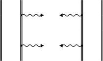
Figure 1: The two-photon emission diagrams in zeroth-order approximation. The double line indicates the electron propagators in the Coulomb field of the nucleus, while the photon emission is depicted by the wavy line with arrow.

In order to calculate the $S$-matrix element of the two-photon transition according to Eq. (11) we expand the two-time Green functions in perturbation series and combine the terms of the same order. The zeroth-order two-photon transition amplitude represented by diagrams in Fig. 1 is given by

$$S^{(0)}_{\gamma_{f_{1}},\gamma_{f_{2}},B;A}=\delta(E_{B}+k_{f_{1}}^{0}+k_{f_{2}}^{0}-E_{A})\oint_{\Gamma_{B}}dE^{\prime}\oint_{\Gamma_{A}}dE\,g^{(0)}_{\gamma_{f_{1}},\gamma_{f_{2}},B;A}(E^{\prime},E,k_{f_{1}}^{0})\,,$$ (18)

where the superscript “$(0)$” indicates the order of the perturbation theory. According to the Feynman rules we obtain

$$g^{(0)}_{\gamma_{f_{1}},\gamma_{f_{2}},B;A}(E^{\prime},E,k_{f_{1}}^{0})\delta(E^{\prime}+k_{f_{1}}^{0}+k_{f_{2}}^{0}-E)$$ (19)

$$= F_{A}F_{B}\sum_{P}(-1)^{P}\int_{-\infty}^{\infty}dp_{1}^{0}dp_{2}^{0}dp_{1}^{\prime 0}dp_{2}^{\prime 0}dq^{0}\,\delta(E-p_{1}^{0}-p_{2}^{0})\,\delta(E^{\prime}-p_{1}^{\prime 0}-p_{2}^{\prime 0})$$

$$\times \left\{\langle Pb_{2}|\frac{i}{2\pi}\sum_{n_{1}}\frac{|n_{1}\rangle\langle n_{1}|}{p_{2}^{\prime 0}-u\varepsilon_{n_{1}}}\frac{2\pi}{i}R_{f_{1}}\delta(p_{2}^{\prime 0}+k_{f_{1}}^{0}-q^{0})\frac{i}{2\pi}\sum_{n_{2}}\frac{|n_{2}\rangle\langle n_{2}|}{q^{0}-u\varepsilon_{n_{2}}}\frac{2\pi}{i}R_{f_{2}}\delta(q^{0}+k_{f_{2}}^{0}-p_{2}^{0})\right.$$

$$\times \frac{i}{2\pi}\sum_{n_{3}}\frac{|n_{3}\rangle\langle n_{3}|}{p_{2}^{0}-u\varepsilon_{n_{3}}}|a_{2}\rangle\langle Pb_{1}|\frac{i}{2\pi}\sum_{n_{4}}\frac{|n_{4}\rangle\langle n_{4}|}{p_{1}^{0}-u\varepsilon_{n_{4}}}|a_{1}\rangle\delta(p_{1}^{\prime 0}-p_{1}^{0})$$

$$+ \langle Pb_{1}|\frac{i}{2\pi}\sum_{n_{1}}\frac{|n_{1}\rangle\langle n_{1}|}{p_{1}^{\prime 0}-u\varepsilon_{n_{1}}}\frac{2\pi}{i}R_{f_{1}}\delta(p_{1}^{\prime 0}+k_{f_{1}}^{0}-q^{0})\frac{i}{2\pi}\sum_{n_{2}}\frac{|n_{2}\rangle\langle n_{2}|}{q^{0}-u\varepsilon_{n_{2}}}\frac{2\pi}{i}R_{f_{2}}\delta(q^{0}+k_{f_{2}}^{0}-p_{1}^{0})$$

$$\times \left.\frac{i}{2\pi}\sum_{n_{3}}\frac{|n_{3}\rangle\langle n_{3}|}{p_{1}^{0}-u\varepsilon_{n_{3}}}|a_{1}\rangle\langle Pb_{2}|\frac{i}{2\pi}\sum_{n_{4}}\frac{|n_{4}\rangle\langle n_{4}|}{p_{2}^{0}-u\varepsilon_{n_{4}}}|a_{2}\rangle\delta(p_{2}^{\prime 0}-p_{2}^{0})+(f_{1}\leftrightarrow f_{2})\right\}$$

$$= \frac{i}{2\pi}\frac{\delta(E^{\prime}+k_{f_{1}}^{0}+k_{f_{2}}^{0}-E)}{(E^{\prime}-E_{B}^{(0)})(E-E_{A}^{(0)})}F_{A}F_{B}\sum_{P}(-1)^{P}\sum_{n}\left\{\frac{\langle Pb_{2}|R_{f_{1}}|n\rangle\langle n|R_{f_{2}}|a_{2}\rangle\delta_{Pb_{1}a_{1}}}{E^{\prime}-\varepsilon_{a_{1}}+k_{f_{1}}^{0}-\varepsilon_{n}}\right.$$

$$+ \left.\frac{\langle Pb_{1}|R_{f_{1}}|n\rangle\langle n|R_{f_{2}}|a_{1}\rangle\delta_{Pb_{2}a_{2}}}{E^{\prime}-\varepsilon_{a_{2}}+k_{f_{1}}^{0}-\varepsilon_{n}}+(f_{1}\leftrightarrow f_{2})\right\}\,,$$

where $R_{f}$ is the transition operator, $R_{f}=e\alpha_{\nu}A_{f}^{\nu*}$, $\alpha^{\mu}=\gamma^{0}\gamma^{\mu}=(1,\bm{\alpha})$, $E_{A}^{(0)}=\varepsilon_{a_{1}}+\varepsilon_{a_{2}}$ and $E_{B}^{(0)}=\varepsilon_{b_{1}}+\varepsilon_{b_{2}}$, $u=1-i0$ preserves the proper treatment of poles of the electron propagators, and the shorthand notation $(f_{1}\leftrightarrow f_{2})$ stands for the contributions with interchanged photons $f_{1}$ and $f_{2}$. Substituting this expression into Eq. (18) and integrating over $E$ and $E^{\prime}$ one obtains

$$\tau_{\gamma_{f_{1}},\gamma_{f_{2}},B;A}^{(0)} = -F_{A}F_{B}\sum_{P}(-1)^{P}\sum_{n}\left\{\frac{\langle Pb_{2}|R_{f_{1}}|n\rangle\langle n|R_{f_{2}}|a_{2}\rangle\delta_{Pb_{1}a_{1}}}{\varepsilon_{Pb_{2}}+k_{f_{1}}^{0}-\varepsilon_{n}}\right.$$ (20)

$$+ \left.\frac{\langle Pb_{1}|R_{f_{1}}|n\rangle\langle n|R_{f_{2}}|a_{1}\rangle\delta_{Pb_{2}a_{2}}}{\varepsilon_{Pb_{1}}+k_{f_{1}}^{0}-\varepsilon_{n}}+(f_{1}\leftrightarrow f_{2})\right\}\,.$$

The corresponding differential transition probability is given by

$$dW_{B;A}^{(0)}(k_{f_{1}},\epsilon_{f_{1}},k_{f_{2}},\epsilon_{f_{2}})=2\pi|\tau_{\gamma_{f_{1}},\gamma_{f_{2}},B;A}^{(0)}|^{2}\delta(E_{B}^{(0)}+k_{f_{1}}^{0}+k_{f_{2}}^{0}-E_{A}^{(0)})d{\bf k}_{f_{1}}d{\bf k}_{f_{2}}\,.$$ (21)

Summing over the photon polarizations and integrating over the photon energies and angles one obtains the total decay rate

$$W_{B;A}^{(0)}=\frac{1}{2}\int_{0}^{\Delta^{(0)}_{AB}}dk_{f_{1}}^{0}\,(k_{f_{1}}^{0})^{2}(\Delta^{(0)}_{AB}-k_{f_{1}}^{0})^{2}\,2\pi\sum_{\epsilon_{f_{1}},\epsilon_{f_{2}}}\int d\Omega_{k_{f_{1}}}d\Omega_{k_{f_{2}}}|\tau_{\gamma_{f_{1}},\gamma_{f_{2}},B;A}^{(0)}|^{2}\,,$$ (22)

where $\Delta^{(0)}_{AB}=E_{A}^{(0)}-E_{B}^{(0)}$. Eqs. (21) and (22) together with Eq. (20) describe the zeroth-order differential and total two-photon transition probabilities, respectively. They coincide with the corresponding formulas employed for the calculation of the two-photon decay rates in He-like ions Drake (1986); Derevianko and Johnson (1997); Labzowsky and Shonin (2004); Surzhykov et al. (2010) in the independent particle model approximation.

II.2 First-order interelectronic-interaction correction

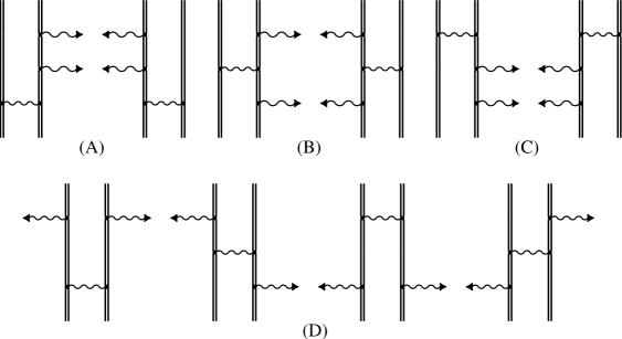
Figure 2: Feynman diagrams representing the first-order interelectronic-interaction corrections to the two-photon emission. Notations are the same as in Fig. 1.

With the formalism outlined above, we are ready now to derive the first-order interelectronic-interaction corrections to the two-photon transition amplitude, which are defined by diagrams depicted in Fig. 2. According to Eq. (11) we start from

$$S^{(1)}_{\gamma_{f_{1}},\gamma_{f_{2}},B;A} = \delta(E_{B}+k_{f_{1}}^{0}+k_{f_{2}}^{0}-E_{A})\left[\oint_{\Gamma_{B}}dE^{\prime}\oint_{\Gamma_{A}}dE\,g^{(1)}_{\gamma_{f_{1}},\gamma_{f_{2}},B;A}(E^{\prime},E,k_{f_{1}}^{0})\right.$$ (23)

$$- \left.\frac{1}{2}\oint_{\Gamma_{B}}dE^{\prime}\oint_{\Gamma_{A}}dE\,g^{(0)}_{\gamma_{f_{1}},\gamma_{f_{2}},B;A}(E^{\prime},E,k_{f_{1}}^{0})\;\left(\frac{1}{2\pi i}\oint_{\Gamma_{A}}dE\,g_{AA}^{(1)}(E)+\frac{1}{2\pi i}\oint_{\Gamma_{B}}dE\,g_{BB}^{(1)}(E)\right)\right]\,,$$

where $g_{AA}^{(1)}$ and $g_{BB}^{(1)}$ are defined by the first-order interelectronic-interaction diagram depicted in Fig. 3.

Figure 3: One-photon exchange diagram. The photon propagator is represented by the wavy line.

Let us first consider the contribution of the diagrams shown in Fig. 2(A). According to the Feynman rules we obtain

$$g^{(1A)}_{\gamma_{f_{1}},\gamma_{f_{2}},B;A}(E^{\prime},E,k_{f_{1}}^{0})\delta(E^{\prime}+k_{f_{1}}^{0}+k_{f_{2}}^{0}-E)$$ (24)

$$= \left(\frac{i}{2\pi}\right)^{3}F_{A}F_{B}\sum_{P}(-1)^{P}\int_{-\infty}^{\infty}dp_{1}^{0}dp_{2}^{0}dp_{1}^{\prime 0}dp_{2}^{\prime 0}dq_{1}^{0}dq_{2}^{0}d\omega\delta(E-p_{1}^{0}-p_{2}^{0})\delta(E^{\prime}-p_{1}^{\prime 0}-p_{2}^{\prime 0})$$

$$\times \sum_{n_{1},n_{2}}\left\{\frac{\delta(p_{2}^{\prime 0}+k_{f_{1}}^{0}-q_{1}^{0})\delta(q_{1}^{0}+k_{f_{2}}^{0}-q_{2}^{0})\delta(q_{2}^{0}-\omega-p_{2}^{0})\delta(p_{1}^{\prime 0}+\omega-p_{1}^{0})}{(p_{1}^{\prime 0}-u\varepsilon_{Pb_{1}})(p_{2}^{\prime 0}-u\varepsilon_{Pb_{2}})(p_{1}^{0}-u\varepsilon_{a_{1}})(p_{2}^{0}-u\varepsilon_{a_{2}})}\right.$$

$$\times \frac{\langle Pb_{2}|R_{f_{1}}|n_{1}\rangle\langle n_{1}|R_{f_{2}}|n_{2}\rangle\langle Pb_{1}n_{2}|I(\omega)|a_{1}a_{2}\rangle}{(q_{1}^{0}-u\varepsilon_{n_{1}})(q_{2}^{0}-u\varepsilon_{n_{2}})}$$

$$+ \frac{\delta(p_{1}^{\prime 0}+k_{f_{1}}^{0}-q_{1}^{0})\delta(q_{1}^{0}+k_{f_{2}}^{0}-q_{2}^{0})\delta(q_{2}^{0}-\omega-p_{1}^{0})\delta(p_{2}^{\prime 0}+\omega-p_{2}^{0})}{(p_{1}^{\prime 0}-u\varepsilon_{Pb_{1}})(p_{2}^{\prime 0}-u\varepsilon_{Pb_{2}})(p_{1}^{0}-u\varepsilon_{a_{1}})(p_{2}^{0}-u\varepsilon_{a_{2}})}$$

$$\times \left.\frac{\langle Pb_{1}|R_{f_{1}}|n_{1}\rangle\langle n_{1}|R_{f_{2}}|n_{2}\rangle\langle n_{2}Pb_{2}|I(\omega)|a_{1}a_{2}\rangle}{(q_{1}^{0}-u\varepsilon_{n_{1}})(q_{2}^{0}-u\varepsilon_{n_{2}})}+(f_{1}\leftrightarrow f_{2})\right\}\,,$$

where $I(\omega)=e^{2}\alpha^{\mu}\alpha^{\nu}D_{\mu\nu}(\omega)$, and $D_{\mu\nu}(\omega)$ is the photon propagator. Eq. (24) is conveniently divided into irreducible and reducible parts. The reducible part is the one with $\varepsilon_{Pb_{1}}+\varepsilon_{n_{2}}=E_{A}^{(0)}$ in first term and with $\varepsilon_{Pb_{2}}+\varepsilon_{n_{2}}=E_{A}^{(0)}$ in the second term. The irreducible part is the reminder. Thus, we obtain for the irreducible contribution

$$g^{(1A,{\rm irr})}_{\gamma_{f_{1}},\gamma_{f_{2}},B;A}(E^{\prime},E,k_{f_{1}}^{0})$$ (25)

$$= \left(\frac{i}{2\pi}\right)^{3}F_{A}F_{B}\sum_{P}(-1)^{P}\int_{-\infty}^{\infty}dp^{0}dp^{\prime 0}\frac{1}{(E^{\prime}-E_{B}^{(0)})(E-E_{A}^{(0)})}$$

$$\times \left\{\sum_{n_{1},n_{2}}^{\varepsilon_{Pb_{1}}+\varepsilon_{n_{2}}\neq E_{A}^{(0)}}\left(\frac{1}{p^{0}-u\varepsilon_{a_{1}}}+\frac{1}{E-p^{0}-u\varepsilon_{a_{2}}}\right)\left(\frac{1}{p^{\prime 0}-u\varepsilon_{Pb_{1}}}+\frac{1}{E^{\prime}-p^{\prime 0}-u\varepsilon_{Pb_{2}}}\right)\right.$$

$$\times \frac{\langle Pb_{2}|R_{f_{1}}|n_{1}\rangle\langle n_{1}|R_{f_{2}}|n_{2}\rangle\langle Pb_{1}n_{2}|I(p^{0}-p^{\prime 0})|a_{1}a_{2}\rangle}{(E^{\prime}-p^{\prime 0}+k_{f_{1}}^{0}-u\varepsilon_{n_{1}})(E-p^{\prime 0}-u\varepsilon_{n_{2}})}$$

$$+ \sum_{n_{1},n_{2}}^{\varepsilon_{Pb_{2}}+\varepsilon_{n_{2}}\neq E_{A}^{(0)}}\left(\frac{1}{p^{0}-u\varepsilon_{a_{2}}}+\frac{1}{E-p^{0}-u\varepsilon_{a_{1}}}\right)\left(\frac{1}{p^{\prime 0}-u\varepsilon_{Pb_{2}}}+\frac{1}{E^{\prime}-p^{\prime 0}-u\varepsilon_{Pb_{1}}}\right)$$

$$\times \left.\frac{\langle Pb_{1}|R_{f_{1}}|n_{1}\rangle\langle n_{1}|R_{f_{2}}|n_{2}\rangle\langle n_{2}Pb_{2}|I(p^{0}-p^{\prime 0})|a_{1}a_{2}\rangle}{(E^{\prime}-p^{\prime 0}+k_{f_{1}}^{0}-u\varepsilon_{n_{1}})(E-p^{\prime 0}-u\varepsilon_{n_{2}})}+(f_{1}\leftrightarrow f_{2})\right\}\,,$$

and for the corresponding reducible one

$$g^{(1A,{\rm red})}_{\gamma_{f_{1}},\gamma_{f_{2}},B;A}(E^{\prime},E,k_{f_{1}}^{0})$$ (26)

$$= \left(\frac{i}{2\pi}\right)^{3}F_{A}F_{B}\sum_{P}(-1)^{P}\int_{-\infty}^{\infty}dp^{0}dp^{\prime 0}\frac{1}{(E^{\prime}-E_{B}^{(0)})(E-E_{A}^{(0)})}$$

$$\times \Biggl{\{}\sum_{n_{1},n_{2}}^{\varepsilon_{Pb_{1}}+\varepsilon_{n_{2}}=E_{A}^{(0)}}\left(\frac{1}{p^{0}-u\varepsilon_{a_{1}}}+\frac{1}{E-p^{0}-u\varepsilon_{a_{2}}}\right)\left[\frac{1}{E-E_{A}^{(0)}}\left(\frac{1}{p^{\prime 0}-u\varepsilon_{Pb_{1}}}+\frac{1}{E-p^{\prime 0}-u\varepsilon_{n_{2}}}\right)\right.$$

$$+ \left.\frac{1}{(E^{\prime}-p^{\prime 0}-u\varepsilon_{Pb_{2}})(E-p^{\prime 0}-u\varepsilon_{n_{2}})}\right]\frac{\langle Pb_{2}|R_{f_{1}}|n_{1}\rangle\langle n_{1}|R_{f_{2}}|n_{2}\rangle\langle Pb_{1}n_{2}|I(p^{0}-p^{\prime 0})|a_{1}a_{2}\rangle}{E^{\prime}-p^{\prime 0}+k_{f_{1}}^{0}-u\varepsilon_{n_{1}}}$$

$$+ \sum_{n_{1},n_{2}}^{\varepsilon_{Pb_{2}}+\varepsilon_{n_{2}}=E_{A}^{(0)}}\left(\frac{1}{p^{0}-u\varepsilon_{a_{2}}}+\frac{1}{E-p^{0}-u\varepsilon_{a_{1}}}\right)\left[\frac{1}{E-E_{A}^{(0)}}\left(\frac{1}{p^{\prime 0}-u\varepsilon_{Pb_{2}}}+\frac{1}{E-p^{\prime 0}-u\varepsilon_{n_{2}}}\right)\right.$$

$$+ \left.\frac{1}{(E^{\prime}-p^{\prime 0}-u\varepsilon_{Pb_{1}})(E-p^{\prime 0}-u\varepsilon_{n_{2}})}\right]\frac{\langle Pb_{1}|R_{f_{1}}|n_{1}\rangle\langle n_{1}|R_{f_{2}}|n_{2}\rangle\langle n_{2}Pb_{2}|I(p^{0}-p^{\prime 0})|a_{1}a_{2}\rangle}{E^{\prime}-p^{\prime 0}+k_{f_{1}}^{0}-u\varepsilon_{n_{1}}}$$

$$+ (f_{1}\leftrightarrow f_{2})\Biggr{\}}\,.$$

The expression in curly braces of Eq. (25) is a regular function of $E$ or $E^{\prime}$ when $E\approx E_{A}^{(0)}$ and $E^{\prime}\approx E_{B}^{(0)}$. Substituting Eq. (25) into Eq. (23) and integrating over $E$ and $E^{\prime}$ we find

$$\tau_{\gamma_{f_{1}},\gamma_{f_{2}},B;A}^{(1A,{\rm irr})} = -F_{A}F_{B}\sum_{P}(-1)^{P}\left\{\sum_{n_{1},n_{2}}^{\varepsilon_{Pb_{1}}+\varepsilon_{n_{2}}\neq E_{A}^{(0)}}\frac{\langle Pb_{2}|R_{f_{1}}|n_{1}\rangle\langle n_{1}|R_{f_{2}}|n_{2}\rangle\langle Pb_{1}n_{2}|I(\varepsilon_{a_{1}}-\varepsilon_{Pb_{1}})|a_{1}a_{2}\rangle}{(\varepsilon_{Pb_{2}}+k_{f_{1}}^{0}-\varepsilon_{n_{1}})(E_{A}^{(0)}-\varepsilon_{Pb_{1}}-\varepsilon_{n_{2}})}\right.$$ (27)

$$+ \left.\sum_{n_{1},n_{2}}^{\varepsilon_{Pb_{2}}+\varepsilon_{n_{2}}\neq E_{A}^{(0)}}\frac{\langle Pb_{1}|R_{f_{1}}|n_{1}\rangle\langle n_{1}|R_{f_{2}}|n_{2}\rangle\langle n_{2}Pb_{2}|I(\varepsilon_{a_{2}}-\varepsilon_{Pb_{2}})|a_{1}a_{2}\rangle}{(\varepsilon_{Pb_{1}}+k_{f_{1}}^{0}-\varepsilon_{n_{1}})(E_{A}^{(0)}-\varepsilon_{Pb_{2}}-\varepsilon_{n_{2}})}+(f_{1}\leftrightarrow f_{2})\right\}\,.$$

A similar calculation for the diagrams shown in Figs. 2(B)-2(D) yields

$$\tau_{\gamma_{f_{1}},\gamma_{f_{2}},B;A}^{(1B)} = -F_{A}F_{B}\sum_{P}(-1)^{P}\left\{\sum_{n_{1},n_{2}}\frac{\langle Pb_{2}|R_{f_{1}}|n_{1}\rangle\langle Pb_{1}n_{1}|I(\varepsilon_{a_{1}}-\varepsilon_{Pb_{1}})|a_{1}n_{2}\rangle\langle n_{2}|R_{f_{2}}|a_{2}\rangle}{(\varepsilon_{Pb_{2}}+k_{f_{1}}^{0}-\varepsilon_{n_{1}})(E_{B}^{(0)}-\varepsilon_{a_{1}}+k_{f_{1}}^{0}-\varepsilon_{n_{2}})}\right.$$ (28)

$$+ \left.\sum_{n_{1},n_{2}}\frac{\langle Pb_{1}|R_{f_{1}}|n_{1}\rangle\langle n_{1}Pb_{2}|I(\varepsilon_{a_{2}}-\varepsilon_{Pb_{2}})|n_{2}a_{2}\rangle\langle n_{2}|R_{f_{2}}|a_{1}\rangle}{(\varepsilon_{Pb_{1}}+k_{f_{1}}^{0}-\varepsilon_{n_{1}})(E_{B}^{(0)}-\varepsilon_{a_{2}}+k_{f_{1}}^{0}-\varepsilon_{n_{2}})}+(f_{1}\leftrightarrow f_{2})\right\}\,,$$

$$\tau_{\gamma_{f_{1}},\gamma_{f_{2}},B;A}^{(1C,{\rm irr})} = -F_{A}F_{B}\sum_{P}(-1)^{P}\left\{\sum_{n_{1},n_{2}}^{\varepsilon_{a_{1}}+\varepsilon_{n_{1}}\neq E_{B}^{(0)}}\frac{\langle Pb_{1}Pb_{2}|I(\varepsilon_{a_{1}}-\varepsilon_{Pb_{1}})|a_{1}n_{1}\rangle\langle n_{1}|R_{f_{1}}|n_{2}\rangle\langle n_{2}|R_{f_{2}}|a_{2}\rangle}{(E_{B}^{(0)}-\varepsilon_{a_{1}}-\varepsilon_{n_{1}})(E_{B}^{(0)}-\varepsilon_{a_{1}}+k_{f_{1}}^{0}-\varepsilon_{n_{2}})}\right.$$ (29)

$$+ \left.\sum_{n_{1},n_{2}}^{\varepsilon_{a_{2}}+\varepsilon_{n_{1}}\neq E_{B}^{(0)}}\frac{\langle Pb_{1}Pb_{2}|I(\varepsilon_{a_{2}}-\varepsilon_{Pb_{2}})|n_{1}a_{2}\rangle\langle n_{1}|R_{f_{1}}|n_{2}\rangle\langle n_{2}|R_{f_{2}}|a_{1}\rangle}{(E_{B}^{(0)}-\varepsilon_{a_{2}}-\varepsilon_{n_{1}})(E_{B}^{(0)}-\varepsilon_{a_{2}}+k_{f_{1}}^{0}-\varepsilon_{n_{2}})}+(f_{1}\leftrightarrow f_{2})\right\}\,,$$

$$\tau_{\gamma_{f_{1}},\gamma_{f_{2}},B;A}^{(1D)} = -F_{A}F_{B}\sum_{P}(-1)^{P}\left\{\sum_{n_{1},n_{2}}\frac{\langle Pb_{1}|R_{f_{1}}|n_{1}\rangle\langle Pb_{2}|R_{f_{2}}|n_{2}\rangle\langle n_{1}n_{2}|I(\varepsilon_{a_{1}}-\varepsilon_{Pb_{1}}-k_{f_{1}}^{0})|a_{1}a_{2}\rangle}{(\varepsilon_{Pb_{1}}+k_{f_{1}}^{0}-\varepsilon_{n_{1}})(E_{A}^{(0)}-\varepsilon_{Pb_{1}}-k_{f_{1}}^{0}-\varepsilon_{n_{2}})}\right.$$ (30)

$$+ \sum_{n_{1},n_{2}}\frac{\langle Pb_{1}|R_{f_{1}}|n_{1}\rangle\langle n_{1}Pb_{2}|I(\varepsilon_{a_{1}}-\varepsilon_{Pb_{1}}-k_{f_{1}}^{0})|a_{1}n_{2}\rangle\langle n_{2}|R_{f_{2}}|a_{2}\rangle}{(\varepsilon_{Pb_{1}}+k_{f_{1}}^{0}-\varepsilon_{n_{1}})(E_{B}^{(0)}-\varepsilon_{a_{1}}+k_{f_{1}}^{0}-\varepsilon_{n_{2}})}$$

$$+ \sum_{n_{1},n_{2}}\frac{\langle Pb_{1}Pb_{2}|I(\varepsilon_{a_{1}}-\varepsilon_{Pb_{1}}-k_{f_{1}}^{0})|n_{1}n_{2}\rangle\langle n_{1}|R_{f_{1}}|a_{1}\rangle\langle n_{2}|R_{f_{2}}|a_{2}\rangle}{(\varepsilon_{a_{1}}-k_{f_{1}}^{0}-\varepsilon_{n_{1}})(E_{B}^{(0)}-\varepsilon_{a_{1}}+k_{f_{1}}^{0}-\varepsilon_{n_{2}})}$$

$$+ \left.\sum_{n_{1},n_{2}}\frac{\langle Pb_{2}|R_{f_{2}}|n_{2}\rangle\langle Pb_{1}n_{2}|I(\varepsilon_{a_{1}}-\varepsilon_{Pb_{1}}-k_{f_{1}}^{0})|n_{1}a_{2}\rangle\langle n_{1}|R_{f_{1}}|a_{1}\rangle}{(\varepsilon_{a_{1}}-k_{f_{1}}^{0}-\varepsilon_{n_{1}})(E_{A}^{(0)}-\varepsilon_{Pb_{1}}-k_{f_{1}}^{0}-\varepsilon_{n_{2}})}+(f_{1}\leftrightarrow f_{2})\right\}\,.$$

In the case under consideration only the diagrams depicted in Figs. 2(A) and 2(C) possess reducible parts. For the reducible contribution coming from the 2(A) diagrams we have

$$\tau_{\gamma_{f_{1}},\gamma_{f_{2}},B;A}^{(1A,{\rm red})} = F_{A}F_{B}\sum_{P}(-1)^{P}\sum_{n}\left\{\frac{\langle Pb_{2}|R_{f_{2}}|n\rangle\langle n|R_{f_{1}}|a_{2}\rangle\delta_{Pb_{1}a_{1}}}{(\varepsilon_{a_{2}}-k_{f_{1}}^{0}-\varepsilon_{n})^{2}}+\frac{\langle Pb_{1}|R_{f_{2}}|n\rangle\langle n|R_{f_{1}}|a_{1}\rangle\delta_{Pb_{2}a_{2}}}{(\varepsilon_{a_{1}}-k_{f_{1}}^{0}-\varepsilon_{n})^{2}}\right\}\Delta E_{A}^{(1)}$$ (31)

$$- \frac{i}{2\pi}\tau_{\gamma_{f_{1}},\gamma_{f_{2}},B;A}^{(0)}F_{A^{\prime}}F_{A^{\prime\prime}}\int_{-\infty}^{\infty}dp^{0}\left[\frac{\langle a^{\prime}_{1}a^{\prime}_{2}|I(p^{0})|a^{\prime\prime}_{1}a^{\prime\prime}_{2}\rangle}{(p^{0}+i0)^{2}}-\frac{\langle a^{\prime}_{2}a^{\prime}_{1}|I(p^{0})|a^{\prime\prime}_{1}a^{\prime\prime}_{2}\rangle}{(p^{0}-\Delta_{A}+i0)^{2}}\right]\,,$$

where $\Delta E_{A}^{(1)}=F_{A^{\prime}}F_{A^{\prime\prime}}\sum_{P}(-1)^{P}\langle Pa^{\prime}_{1}Pa^{\prime}_{2}|I(\varepsilon_{Pa^{\prime}_{1}}-\varepsilon_{a^{\prime\prime}_{1}})|a^{\prime\prime}_{1}a^{\prime\prime}_{2}\rangle$ is the one-photon exchange correction to the state $A$ and $\Delta_{A}=\varepsilon_{a_{2}}-\varepsilon_{a_{1}}$. Combining this term together with the reducible part of the 2(C) diagrams and with the second term in formula (23), we obtain the total reducible contribution:

$$\tau_{\gamma_{f_{1}},\gamma_{f_{2}},B;A}^{(1,{\rm red})} = F_{A}F_{B}\sum_{P}(-1)^{P}\sum_{n}\left\{\frac{\langle Pb_{2}|R_{f_{1}}|n\rangle\langle n|R_{f_{2}}|a_{2}\rangle\delta_{Pb_{1}a_{1}}}{(\varepsilon_{Pb_{2}}+k_{f_{1}}^{0}-\varepsilon_{n})^{2}}\Delta E_{B}^{(1)}+\frac{\langle Pb_{1}|R_{f_{1}}|n\rangle\langle n|R_{f_{2}}|a_{1}\rangle\delta_{Pb_{2}a_{2}}}{(\varepsilon_{Pb_{1}}+k_{f_{1}}^{0}-\varepsilon_{n})^{2}}\Delta E_{B}^{(1)}\right.$$ (32)

$$+ \left.\frac{\langle Pb_{2}|R_{f_{2}}|n\rangle\langle n|R_{f_{1}}|a_{2}\rangle\delta_{Pb_{1}a_{1}}}{(\varepsilon_{a_{2}}-k_{f_{1}}^{0}-\varepsilon_{n})^{2}}\Delta E_{A}^{(1)}+\frac{\langle Pb_{1}|R_{f_{2}}|n\rangle\langle n|R_{f_{1}}|a_{1}\rangle\delta_{Pb_{2}a_{2}}}{(\varepsilon_{a_{1}}-k_{f_{1}}^{0}-\varepsilon_{n})^{2}}\Delta E_{A}^{(1)}\right\}$$

$$+ \frac{1}{2}\tau_{\gamma_{f_{1}},\gamma_{f_{2}},B;A}^{(0)}\left[F_{A^{\prime}}F_{A^{\prime\prime}}\langle a^{\prime}_{2}a^{\prime}_{1}|I^{\prime}(\Delta_{A})|a^{\prime\prime}_{1}a^{\prime\prime}_{2}\rangle+F_{B^{\prime}}F_{B^{\prime\prime}}\langle b^{\prime}_{2}b^{\prime}_{1}|I^{\prime}(\Delta_{B})|b^{\prime\prime}_{1}b^{\prime\prime}_{2}\rangle\right]\,,$$

where $\Delta E_{B}^{(1)}$ and $\Delta_{B}$ are defined similar as $\Delta E_{A}^{(1)}$ and $\Delta_{A}$, $I^{\prime}(\Delta)=[dI(\omega)/d\omega]_{\omega=\Delta}$. The final expression for $\tau_{\gamma_{f_{1}},\gamma_{f_{2}},B;A}^{(1)}$ is given by the sum of Eqs. (27)-(30), and (32):

$$\tau_{\gamma_{f_{1}},\gamma_{f_{2}},B;A}^{(1)}=\tau_{\gamma_{f_{1}},\gamma_{f_{2}},B;A}^{(1A,{\rm irr})}+\tau_{\gamma_{f_{1}},\gamma_{f_{2}},B;A}^{(1B)}+\tau_{\gamma_{f_{1}},\gamma_{f_{2}},B;A}^{(1C,{\rm irr})}+\tau_{\gamma_{f_{1}},\gamma_{f_{2}},B;A}^{(1D)}+\tau_{\gamma_{f_{1}},\gamma_{f_{2}},B;A}^{(1,{\rm red})}\,.$$ (33)

Finally, the first-order interelectronic-interaction corrections to the differential and total transition probabilities can be expressed according to the following equations

$$dW_{B;A}^{(1)}(k_{f_{1}},\epsilon_{f_{1}},k_{f_{2}},\epsilon_{f_{2}}) = 4\pi{\rm Re}\left\{\tau_{\gamma_{f_{1}},\gamma_{f_{2}},B;A}^{(0)*}\tau_{\gamma_{f_{1}},\gamma_{f_{2}},B;A}^{(1)}\right\}\delta(E_{B}^{(1)}+k_{f_{1}}^{0}+k_{f_{2}}^{0}-E_{A}^{(1)})d{\bf k}_{f_{1}}d{\bf k}_{f_{2}}$$ (34)

$$+ \Delta dW_{B;A}^{(0)}(k_{f_{1}},\epsilon_{f_{1}},k_{f_{2}},\epsilon_{f_{2}})\,,$$

$$W_{B;A}^{(1)}=\frac{1}{2}\int_{0}^{\Delta^{(1)}_{AB}}dk_{f_{1}}^{0}\,(k_{f_{1}}^{0})^{2}(\Delta^{(1)}_{AB}-k_{f_{1}}^{0})^{2}\,4\pi\sum_{\epsilon_{f_{1}},\epsilon_{f_{2}}}\int d\Omega_{k_{f_{1}}}d\Omega_{k_{f_{2}}}{\rm Re}\left\{\tau_{\gamma_{f_{1}},\gamma_{f_{2}},B;A}^{(0)*}\tau_{\gamma_{f_{1}},\gamma_{f_{2}},B;A}^{(1)}\right\}+\Delta W_{B;A}^{(0)}\,,$$ (35)

where $E_{A}^{(1)}=E_{A}^{(0)}+\Delta E_{A}^{(1)}$, $E_{B}^{(1)}=E_{B}^{(0)}+\Delta E_{B}^{(1)}$, $\Delta^{(1)}_{AB}=E_{A}^{(1)}-E_{B}^{(1)}$, and

$$\Delta dW_{B;A}^{(0)}(k_{f_{1}},\epsilon_{f_{1}},k_{f_{2}},\epsilon_{f_{2}})=2\pi|\tau_{\gamma_{f_{1}},\gamma_{f_{2}},B;A}^{(0)}|^{2}\delta(E_{B}^{(1)}+k_{f_{1}}^{0}+k_{f_{2}}^{0}-E_{A}^{(1)})d{\bf k}_{f_{1}}d{\bf k}_{f_{2}}-dW_{B;A}^{(0)}(k_{f_{1}},\epsilon_{f_{1}},k_{f_{2}},\epsilon_{f_{2}})\,,$$ (36)

$$\Delta W_{B;A}^{(0)}=\frac{1}{2}\int_{0}^{\Delta^{(1)}_{AB}}dk_{f_{1}}^{0}\,(k_{f_{1}}^{0})^{2}(\Delta^{(1)}_{AB}-k_{f_{1}}^{0})^{2}\,2\pi\sum_{\epsilon_{f_{1}},\epsilon_{f_{2}}}\int d\Omega_{k_{f_{1}}}d\Omega_{k_{f_{2}}}|\tau_{\gamma_{f_{1}},\gamma_{f_{2}},B;A}^{(0)}|^{2}-W_{B;A}^{(0)}$$ (37)

are the contributions originating from changing the transition energy $\Delta^{(0)}_{AB}$ in the zeroth-order transition probability to the energy $\Delta^{(1)}_{AB}$, which accounts for the interelectronic-interaction correction.

II.3 First-order interelectronic-interaction correction with screening potential

In the previous subsection we presented the formulas for the first-order interelectronic-interaction correction involving electron states and propagators in the external Coulomb potential of the nucleus as the zeroth-order approximation (the original Furry picture). Now we consider an extended Furry picture, which includes a local screening potential in the unperturbed Hamiltonian. Since further we consider the two-photon decays from the single-excited state to the ground state of He-like ions, we construct the screening potential for the initial state $A$ such that it takes into account partly the interelectronic interaction between the electrons $a_{2}$ and $a_{1}$. By employing the extended Furry representation, we already at the zeroth-order level relieve the quasidegeneracy of the $(1s2s)_{J}$ and $(1s2p_{1/2})_{J}$ states, and improve the energy level scheme of the first excited states in high-$Z$ heavy ions. Two different local screening potentials $V_{\rm scr}$ are used: the Kohn-Sham potential and the core-Hartree potential. Both potentials were successfully incorporated in previous calculations Glazov et al. (2006); Volotka et al. (2008b); Trotsenko et al. (2010); Surzhykov et al. (2010).

In the extended Furry picture we solve the Dirac equation with an effective spherically symmetric potential treating the interaction with the external Coulomb potential of the nucleus and the local screening potential exact to all orders. The electron propagators in Figs. 1-3 have to be treated in the effective potential (we indicate this diagrammatically via the triple electron line). The formulas derived in the previous subsection remain formally the same, but keeping in mind that the Dirac spectrum is now generated by solving the Dirac equation with the effective potential. However, additional counterterm diagrams with the extra interaction term $-V_{\rm scr}$ arise. In Figs. 4 and 5 the additional diagrams are depicted, where the extra interaction term $-V_{\rm scr}$ is represented graphically by the symbol $\otimes$.

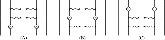
Figure 4: The counterterm diagrams for the first-order interelectronic-interaction corrections to the two-photon emission. The triple lines describe the electron propagators in the effective potential. The symbol $\otimes$ represents the extra interaction term associated with the local screening potential.

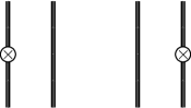
Figure 5: The counterterm diagrams for the one-photon exchange correction. Notations are the same as in Fig. 4.

Thus, according to the Feynman rules we derive the expressions for the counterterm diagrams shown in Figs. 4(A)-4(C)

$$\tau_{\gamma_{f_{1}},\gamma_{f_{2}},B;A}^{(1A,{\rm irr}){\rm ext}} = F_{A}F_{B}\sum_{P}(-1)^{P}\left\{\sum_{n_{1},n_{2}}^{\varepsilon_{n_{2}}\neq\varepsilon_{a_{2}}}\frac{\langle Pb_{2}|R_{f_{1}}|n_{1}\rangle\langle n_{1}|R_{f_{2}}|n_{2}\rangle\langle n_{2}|V_{\rm scr}|a_{2}\rangle\delta_{Pb_{1}a_{1}}}{(\varepsilon_{Pb_{2}}+k_{f_{1}}^{0}-\varepsilon_{n_{1}})(\varepsilon_{a_{2}}-\varepsilon_{n_{2}})}\right.$$ (38)

$$+ \left.\sum_{n_{1},n_{2}}^{\varepsilon_{n_{2}}\neq\varepsilon_{a_{1}}}\frac{\langle Pb_{1}|R_{f_{1}}|n_{1}\rangle\langle n_{1}|R_{f_{2}}|n_{2}\rangle\langle n_{2}|V_{\rm scr}|a_{1}\rangle\delta_{Pb_{2}a_{2}}}{(\varepsilon_{Pb_{1}}+k_{f_{1}}^{0}-\varepsilon_{n_{1}})(\varepsilon_{a_{1}}-\varepsilon_{n_{2}})}+(f_{1}\leftrightarrow f_{2})\right\}\,,$$

$$\tau_{\gamma_{f_{1}},\gamma_{f_{2}},B;A}^{(1B){\rm ext}} = F_{A}F_{B}\sum_{P}(-1)^{P}\left\{\sum_{n_{1},n_{2}}\frac{\langle Pb_{2}|R_{f_{1}}|n_{1}\rangle\langle n_{1}|V_{\rm scr}|n_{2}\rangle\langle n_{2}|R_{f_{2}}|a_{2}\rangle\delta_{Pb_{1}a_{1}}}{(\varepsilon_{Pb_{2}}+k_{f_{1}}^{0}-\varepsilon_{n_{1}})(\varepsilon_{Pb_{2}}+k_{f_{1}}^{0}-\varepsilon_{n_{2}})}\right.$$ (39)

$$+ \left.\sum_{n_{1},n_{2}}\frac{\langle Pb_{1}|R_{f_{1}}|n_{1}\rangle\langle n_{1}|V_{\rm scr}|n_{2}\rangle\langle n_{2}|R_{f_{2}}|a_{1}\rangle\delta_{Pb_{2}a_{2}}}{(\varepsilon_{Pb_{1}}+k_{f_{1}}^{0}-\varepsilon_{n_{1}})(\varepsilon_{Pb_{1}}+k_{f_{1}}^{0}-\varepsilon_{n_{2}})}+(f_{1}\leftrightarrow f_{2})\right\}\,,$$

$$\tau_{\gamma_{f_{1}},\gamma_{f_{2}},B;A}^{(1C,{\rm irr}){\rm ext}} = F_{A}F_{B}\sum_{P}(-1)^{P}\left\{\sum_{n_{1},n_{2}}^{\varepsilon_{n_{1}}\neq\varepsilon_{Pb_{2}}}\frac{\langle Pb_{2}|V_{\rm scr}|n_{1}\rangle\langle n_{1}|R_{f_{1}}|n_{2}\rangle\langle n_{2}|R_{f_{2}}|a_{2}\rangle\delta_{Pb_{1}a_{1}}}{(\varepsilon_{Pb_{2}}-\varepsilon_{n_{1}})(\varepsilon_{Pb_{2}}+k_{f_{1}}^{0}-\varepsilon_{n_{2}})}\right.$$ (40)

$$+ \left.\sum_{n_{1},n_{2}}^{\varepsilon_{n_{1}}\neq\varepsilon_{Pb_{1}}}\frac{\langle Pb_{1}|V_{\rm scr}|n_{1}\rangle\langle n_{1}|R_{f_{1}}|n_{2}\rangle\langle n_{2}|R_{f_{2}}|a_{1}\rangle\delta_{Pb_{2}a_{2}}}{(\varepsilon_{Pb_{1}}-\varepsilon_{n_{1}})(\varepsilon_{Pb_{1}}+k_{f_{1}}^{0}-\varepsilon_{n_{2}})}+(f_{1}\leftrightarrow f_{2})\right\}\,.$$

For the additional reducible contribution we obtain

$$\tau_{\gamma_{f_{1}},\gamma_{f_{2}},B;A}^{(1,{\rm red}){\rm ext}} = -F_{A}F_{B}\sum_{P}(-1)^{P}\sum_{n}\left\{\left[\frac{\langle Pb_{2}|R_{f_{1}}|n\rangle\langle n|R_{f_{2}}|a_{2}\rangle\delta_{Pb_{1}a_{1}}}{(\varepsilon_{Pb_{2}}+k_{f_{1}}^{0}-\varepsilon_{n})^{2}}+\frac{\langle Pb_{1}|R_{f_{1}}|n\rangle\langle n|R_{f_{2}}|a_{1}\rangle\delta_{Pb_{2}a_{2}}}{(\varepsilon_{Pb_{1}}+k_{f_{1}}^{0}-\varepsilon_{n})^{2}}\right]\Delta E_{B}^{(1){\rm ext}}\right.$$ (41)

$$+ \left.\left[\frac{\langle Pb_{2}|R_{f_{2}}|n\rangle\langle n|R_{f_{1}}|a_{2}\rangle\delta_{Pb_{1}a_{1}}}{(\varepsilon_{a_{2}}-k_{f_{1}}^{0}-\varepsilon_{n})^{2}}+\frac{\langle Pb_{1}|R_{f_{2}}|n\rangle\langle n|R_{f_{1}}|a_{1}\rangle\delta_{Pb_{2}a_{2}}}{(\varepsilon_{a_{1}}-k_{f_{1}}^{0}-\varepsilon_{n})^{2}}\right]\Delta E_{A}^{(1){\rm ext}}\right\}\,,$$

where $\Delta E_{A}^{(1){\rm ext}}$ and $\Delta E_{B}^{(1){\rm ext}}$ are the counterterm contributions to the energy of the initial and final states, respectively,

$$\Delta E_{A}^{(1){\rm ext}}=-F_{A^{\prime}}F_{A^{\prime\prime}}\sum_{P}(-1)^{P}(\langle Pa^{\prime}_{1}|V_{\rm scr}|a^{\prime\prime}_{1}\rangle\delta_{Pa^{\prime}_{2}a^{\prime\prime}_{2}}+\langle Pa^{\prime}_{2}|V_{\rm scr}|a^{\prime\prime}_{2}\rangle\delta_{Pa^{\prime}_{1}a^{\prime\prime}_{1}})\,.$$ (42)

Thus, in the extended Furry representation these extra terms have to be added to the corresponding corrections to the transition amplitude as $\tau_{\gamma_{f_{1}},\gamma_{f_{2}},B;A}^{(1A,{\rm irr})}\rightarrow\left(\tau_{\gamma_{f_{1}},\gamma_{f_{2}},B;A}^{(1A,{\rm irr})}+\tau_{\gamma_{f_{1}},\gamma_{f_{2}},B;A}^{(1A,{\rm irr}){\rm ext}}\right)$ , and, similarly, the rest terms. Moreover, in Eqs. (34) and (35) the employed energies $E_{A}^{(1)}$ and $E_{B}^{(1)}$ have to be corrected to the counterterm contributions $E_{A}^{(1)}=E_{A}^{(0)}+\Delta E_{A}^{(1)}+\Delta E_{A}^{(1){\rm ext}}$ and $E_{B}^{(1)}=E_{B}^{(0)}+\Delta E_{B}^{(1)}+\Delta E_{B}^{(1){\rm ext}}$.

III Numerical results and discussion

Now let us turn to the presentation and discussion of our numerical results for the two-photon transitions $2^{1}S_{0}\rightarrow 1^{1}S_{0}$ and $2^{3}S_{1}\rightarrow 1^{1}S_{0}$ in He-like ions. The infinite summations over the complete Dirac spectrum involved in the numerical evaluations are performed employing the finite-basis set method. The B-splines basis set was constructed utilizing the dual kinetic balance approach Shabaev et al. (2004). The homogeneously charged sphere model for the nuclear charge distribution is employed together with the rms radii taken from Ref. Angeli (2004), except for the thorium and uranium ions, for which the recent rms values are taken from Ref. Kozhedub et al. (2008). The Kohn-Sham and core-Hartree screening potentials are employed in the zeroth-order approximation. The Kohn-Sham potentials are constructed for the $2^{1}S_{0}$ state in the case of $2^{1}S_{0}\rightarrow 1^{1}S_{0}$ transition, and for the $2^{3}S_{1}$ state in the case of $2^{3}S_{1}\rightarrow 1^{1}S_{0}$ transition, while the core-Hartree potential is just a Coulomb potential generated by the $1s$ electron. The screening potentials are generated self-consistently by solving the Dirac equation until the energies of the core and valence states become stable on the level of $10^{-9}$. In our final compilation we employ the Kohn-Sham potential as a starting one, since the transition energies are better reproduced in this case. The gauge invariance serves as an accurate check of consistency of the derived formulas and the numerical procedure. We analytically proof the gauge invariance of the obtained formulas. In order to separate out the proper gauge invariant first-order contribution we replace the transition operator $R_{f_{2}}$ with the first two terms of the Taylor expansion in $\tau_{\gamma_{f_{1}},\gamma_{f_{2}},B;A}^{(0)}$, as $R_{f_{2}}(k_{f_{2}}^{0})\simeq R_{f_{2}}(\Delta_{AB}^{(0)}-k_{f_{1}}^{0})+R^{\prime}_{f_{2}}(\Delta_{AB}^{(0)}-k_{f_{1}}^{0})\times\left[\Delta E_{A}^{(1)}-\Delta E_{B}^{(1)}\right]$, and with the first term only in $\tau_{\gamma_{f_{1}},\gamma_{f_{2}},B;A}^{(1)}$, as $R_{f_{2}}(k_{f_{2}}^{0})\simeq R_{f_{2}}(\Delta_{AB}^{(0)}-k_{f_{1}}^{0})$. In the numerical procedure we employ the Feynman and Coulomb gauges for the photon propagator and the velocity and length gauges for the emitted photons and demonstrate the gauge independence of the final results. In Table 1 we present the numerical results for the individual contributions evaluated in the different gauges for He-like thorium. As one can see from the table, the gauge invariance is restored in the final values.

Table 1: Individual contributions to the total two-photon decay rates for the transitions $2^{1}S_{0}\rightarrow 1^{1}S_{0}+2\gamma(\rm E1)$ and $2^{3}S_{1}\rightarrow 1^{1}S_{0}+2\gamma(\rm E1)$ in He-like ²³²Th⁸⁸⁺, in units s^-1. The Kohn-Sham potential has been used as the starting potential. The velocity and length gauges have been employed for the emitted photons, and Feynman and Coulomb gauges for the photon propagator. The more accurate transition energies $\Delta^{(1)}_{2^{1}S_{0};1^{1}S_{0}}=91531$ eV and $\Delta^{(1)}_{2^{3}S_{1};1^{1}S_{0}}=91291$ eV are taken from Ref. Artemyev et al. (2005). Numbers in brackets are powers of ten.

Gauges	$W_{B;A}^{(0)}$	$\Delta W_{B;A}^{(0)}$	$W_{B;A}^{(1,{\rm irr})}$	$W_{B;A}^{(1,{\rm red})}$	$W_{B;A}$
$2^{1}S_{0}\rightarrow 1^{1}S_{0}$
Velocity / Feynman	6.439[12]	-0.0862[12]	0.0165[12]	0.0123[12]	6.381[12]
Length / Feynman	6.439[12]	-0.1610[12]	0.0054[12]	0.0982[12]	6.381[12]
Velocity / Coulomb	6.439[12]	-0.0862[12]	0.0169[12]	0.0119[12]	6.381[12]
Length / Coulomb	6.439[12]	-0.1610[12]	0.0058[12]	0.0978[12]	6.381[12]
$2^{3}S_{1}\rightarrow 1^{1}S_{0}$
Velocity / Feynman	1.686[10]	-0.0972[10]	0.0115[10]	0.0349[10]	1.636[10]
Length / Feynman	1.686[10]	-0.1746[10]	0.0369[10]	0.0868[10]	1.636[10]
Velocity / Coulomb	1.686[10]	-0.0972[10]	0.0114[10]	0.0350[10]	1.636[10]
Length / Coulomb	1.686[10]	-0.1746[10]	0.0369[10]	0.0869[10]	1.636[10]

A detailed discussion of these questions will be presented elsewhere.

In Table 2 we present the zeroth-order and final values of the two-photon decay rates for the transitions $2^{1}S_{0}\rightarrow 1^{1}S_{0}+2\gamma({\rm E1})$ and $2^{3}S_{1}\rightarrow 1^{1}S_{0}+2\gamma({\rm E1})$ in He-like ions. These results include only the dominant 2E1 channel of the two-photon decay. The final results for the total two-photon decay rates are evaluated according to the following formula

$$W_{B;A}=\frac{1}{2}\int_{0}^{\Delta^{(1)}_{AB}}dk_{f_{1}}^{0}\,(k_{f_{1}}^{0})^{2}(\Delta^{(1)}_{AB}-k_{f_{1}}^{0})^{2}\,2\pi\sum_{\epsilon_{f_{1}},\epsilon_{f_{2}}}\int d\Omega_{k_{f_{1}}}d\Omega_{k_{f_{2}}}|\tau_{\gamma_{f_{1}},\gamma_{f_{2}},B;A}^{(0)}+\tau_{\gamma_{f_{1}},\gamma_{f_{2}},B;A}^{(1)}|^{2}\,,$$ (43)

where in $\tau_{\gamma_{f_{1}},\gamma_{f_{2}},B;A}^{(0)}$ and $\tau_{\gamma_{f_{1}},\gamma_{f_{2}},B;A}^{(1)}$, defined by Eq. (20) and Eqs. (33), (38)-(41), respectively, we separate out the terms up to the first order. The transition energies $\Delta^{(1)}_{AB}$ together with the transition amplitudes $\tau_{\gamma_{f_{1}},\gamma_{f_{2}},B;A}^{(1)}$ consistently include the first-order interelectronic-interaction corrections to the two-photon decay rate $W_{B;A}$. However, for high-$Z$ ions it is important also to take into account the radiative corrections. In the framework of QED perturbation theory, one has to evaluate radiative corrections to both the transition energy and the transition amplitude. In order to account partially for the radiative corrections, we employ the more accurate transition energies taken from Ref. Artemyev et al. (2005) for the transition energies $\Delta^{(1)}_{AB}$ in the upper integral limit and in the factor $(\Delta^{(1)}_{AB}-k_{f_{1}}^{0})$ in Eq. (43). Including by this way the more accurate transition energies does not violate the gauge invariance of the result; it just scales the decay rates to another value of the transition energy. The employment of the more accurate transition energies yields corrections that are negligible for intermediate-$Z$, which however become important for high-$Z$ ions.

The results of calculations performed by starting with the Coulomb, core-Hartree, and Kohn-Sham potentials are presented in Table 2. Comparing the zeroth-order values in the Coulomb and screening potentials one can observe that the screening potentials account for a considerable part of electron-electron interaction effects. However, the difference between the zeroth-order results for the core-Hartree and Kohn-Sham potentials is still quite large. Accounting for the first-order interelectronic-interaction correction, we obtain the decay rates $W_{B;A}$, which much less depend on the screening potential. The remaining difference between the final values $W_{B;A}$ in the core-Hartree and Kohn-Sham potentials provides a hint for the uncertainty due to unaccounted second- and higher-order interelectronic-interaction corrections. In Table 2 we also compare the obtained decay rates $W_{B;A}$ with the results of other theoretical calculations. In the case of the $2^{1}S_{0}$ state our decay rates slightly disagree with the rates given by Derevianko and Johnson Derevianko and Johnson (1997). For high-$Z$ ions this can be explained by the radiative corrections, which are included in our transition energies. The comparison with the results obtained by Drake Drake (1986) gives a better agreement within the indicated uncertainty. In the case of the $2^{3}S_{1}$ state the interelectronic interaction affects the two-photon decay rates much stronger, and therefore our accuracy becomes slightly worse. For this case our results are in a fair agreement with those values of Ref. Derevianko and Johnson (1997).

As on can see from Table 2, the final values of the total two-photon decay rates calculated with the core-Hartree and Kohn-Sham potentials are very close to each other. With this in mind, we restrict our further consideration to the calculations performed with the Kohn-Sham screening potential.

Table 2: The zeroth-order and final values of the total two-photon decay rates (2E1 channel only) for the transitions $2^{1}S_{0}\rightarrow 1^{1}S_{0}$ and $2^{3}S_{1}\rightarrow 1^{1}S_{0}$ in He-like ions starting with the Coulomb, core-Hartree, and Kohn-Sham potentials, in units s^-1. Comparison with other theoretical calculations is also made. Numbers in brackets denote powers of ten.

	Coulomb	core-Hartree		Kohn-Sham		Other theor.
$Z$	$W_{B;A}^{(0)}$	$W_{B;A}^{(0)}$	$W_{B;A}$	$W_{B;A}^{(0)}$	$W_{B;A}$	Ref. Derevianko and Johnson (1997)	Ref. Drake (1986)
$2^{1}S_{0}\rightarrow 1^{1}S_{0}$
30	1.164[10]	9.944[09]	9.903[09]	1.006[10]	9.900[09]	9.938[09]	9.88(3)[09]
50	2.370[11]	2.163[11]	2.152[11]	2.177[11]	2.152[11]	2.164[11]	2.15(1)[11]
70	1.655[12]	1.554[12]	1.545[12]	1.560[12]	1.544[12]	1.556[12]	1.55(1)[12]
90	6.728[12]	6.421[12]	6.382[12]	6.439[12]	6.381[12]	6.439[12]	6.41(6)[12]
92	7.580[12]	7.242[12]	7.199[12]	7.262[12]	7.199[12]	7.265[12]	7.24(8)[12]
$2^{3}S_{1}\rightarrow 1^{1}S_{0}$
30	9.06[05]	4.64[05]	4.15[05]	4.42[05]	4.13[05]	4.17[05]
50	1.02[08]	7.33[07]	6.88[07]	7.16[07]	6.85[07]	6.88[07]
70	2.13[09]	1.74[09]	1.67[09]	1.72[09]	1.66[09]	1.66[09]
90	1.96[10]	1.70[10]	1.64[10]	1.69[10]	1.64[10]	1.63[10]
92	2.38[10]	2.07[10]	1.99[10]	2.05[10]	1.99[10]	1.98[10]

Beyond the dominant 2E1 decay channel we consider also the higher-multipole contributions to the two-photon decay rates. In Table 3 we present the contributions of higher multipoles calculated in the zeroth-order approximation. In the case of the $2^{1}S_{0}$ state the contribution to the total two-photon decay rate arises only from the photons with the same multipole numbers. The correction due to the higher multipoles rapidly increases with $Z$, but even for $Z=92$ it is by a factor $10^{3}$ smaller than the dominant 2E1 decay rate. Unlike the $2^{1}S_{0}$ state, in the case of the two-photon $2^{3}S_{1}\rightarrow 1^{1}S_{0}$ transition the higher multipoles decay rates are relatively large, as was first indicated by Dunford Dunford (2004). Our results for the E1M2 decay rate are in reasonable agreement with those of Ref. Dunford (2004). Moreover, we also evaluate the 2M1 channel, which contribution becomes comparable with the E1M2 for high-$Z$ ions. The contributions of higher multipoles are included in our final compilations.

Table 3: Contributions of the higher multipoles (MP) to the total two-photon decay rates included in the zeroth-order approximation, in units s^-1. Numbers in brackets denote powers of ten.

MP	$Z=30$	$Z=50$	$Z=70$	$Z=90$	$Z=92$
$2^{1}S_{0}\rightarrow 1^{1}S_{0}$
M1M1	1.40[04]	2.65[06]	8.56[07]	1.14[09]	1.43[09]
E2E2	4.74[03]	8.19[05]	2.33[07]	2.71[08]	3.35[08]
$2^{3}S_{1}\rightarrow 1^{1}S_{0}$
E1M2	7.57[04]	1.32[07]	3.79[08]	4.51[09]	5.59[09]
		1.26[07]a	3.62[08]a	4.30[09]a	5.32[09]a
M1M1	1.58[01]	2.46[04]	3.33[06]	1.46[08]	2.05[08]

^a Ref. Dunford (2004).

In Table 4 we compare the theoretical and experimental two-photon decay rates of the $2^{1}S_{0}$ state. As one can see from the table, for Br³³⁺ and Nb³⁹⁺ ions the theory is in a good agreement with the experiment, but for Ni²⁶⁺ and Kr³⁴⁺ ions all theoretical calculations predict the values being slightly larger than the experimental results. In the worst case of the Kr³⁴⁺ ion this difference amounts to about two standard deviations.

Table 4: Comparison of theory and experiment for the two-photon decay rates of the $2^{1}S_{0}$ state in He-like ions, in units s^-1. Numbers in brackets denote powers of ten.

$Z$	Expt.	This work	Ref. Derevianko and Johnson (1997)	Ref. Drake (1986)
28	6.406(66)[09]a	6.493[09]	6.517[09]	6.482(21)[09]
35	2.543(21)[10]b	2.529[10]	2.540[10]
36	2.934(30)[10]c	2.999[10]	3.012[10]	2.993(12)[10]
41	6.52(26)[10]d	6.572[10]	6.604[10]

^a Ref. Dunford et al. (1993b).           ^c Ref. Marrus et al. (1986).
^b Ref. Dunford et al. (1993a).           ^d Ref. Simionovici et al. (1993).

Finally, in Table 5 we present our total two-photon decay rates for the transitions $2^{1}S_{0}\rightarrow 1^{1}S_{0}$ and $2^{3}S_{1}\rightarrow 1^{1}S_{0}$.

Table 5: The total two-photon decay rates for the transitions $2^{1}S_{0}\rightarrow 1^{1}S_{0}$ and $2^{3}S_{1}\rightarrow 1^{1}S_{0}$ in He-like ions, in units s^-1. The transition energies are taken from Ref. Artemyev et al. (2005). Numbers in brackets denote powers of ten.

$Z$	$2^{1}S_{0}$	$2^{3}S_{1}$	$Z$	$2^{1}S_{0}$	$2^{3}S_{1}$
28	6.493[09]	2.40[05]	61	6.948[11]	5.56[08]
29	8.048[09]	3.44[05]	62	7.640[11]	6.49[08]
30	9.900[09]	4.88[05]	63	8.388[11]	7.56[08]
31	1.209[10]	6.84[05]	64	9.193[11]	8.77[08]
32	1.467[10]	9.46[05]	65	1.006[12]	1.02[09]
33	1.769[10]	1.30[06]	66	1.099[12]	1.17[09]
34	2.121[10]	1.76[06]	67	1.199[12]	1.35[09]
35	2.529[10]	2.36[06]	68	1.307[12]	1.56[09]
36	2.999[10]	3.13[06]	69	1.422[12]	1.79[09]
37	3.539[10]	4.13[06]	70	1.545[12]	2.04[09]
38	4.158[10]	5.40[06]	71	1.676[12]	2.33[09]
39	4.863[10]	7.01[06]	72	1.816[12]	2.66[09]
40	5.664[10]	9.04[06]	73	1.966[12]	3.03[09]
41	6.572[10]	1.16[07]	74	2.125[12]	3.44[09]
42	7.595[10]	1.47[07]	75	2.294[12]	3.90[09]
43	8.747[10]	1.86[07]	76	2.474[12]	4.41[09]
44	1.004[11]	2.33[07]	77	2.665[12]	4.98[09]
45	1.148[11]	2.91[07]	78	2.867[12]	5.61[09]
46	1.310[11]	3.61[07]	79	3.082[12]	6.32[09]
47	1.489[11]	4.46[07]	80	3.309[12]	7.10[09]
48	1.688[11]	5.49[07]	81	3.549[12]	7.96[09]
49	1.908[11]	6.71[07]	82	3.803[12]	8.92[09]
50	2.152[11]	8.18[07]	83	4.071[12]	9.98[09]
51	2.420[11]	9.91[07]	84	4.353[12]	1.11[10]
52	2.715[11]	1.20[08]	85	4.650[12]	1.24[10]
53	3.039[11]	1.44[08]	86	4.963[12]	1.38[10]
54	3.394[11]	1.73[08]	87	5.292[12]	1.54[10]
55	3.783[11]	2.06[08]	88	5.638[12]	1.71[10]
56	4.206[11]	2.45[08]	89	6.002[12]	1.90[10]
57	4.668[11]	2.90[08]	90	6.383[12]	2.10[10]
58	5.171[11]	3.43[08]	91	6.782[12]	2.32[10]
59	5.716[11]	4.04[08]	92	7.200[12]	2.57[10]
60	6.308[11]	4.75[08]

Besides the total decay rates, we present the spectral-distribution functions $dW_{B;A}/dy$ for the two-photon transitions $2^{1}S_{0}\rightarrow 1^{1}S_{0}$ and $2^{3}S_{1}\rightarrow 1^{1}S_{0}$ in Tables 6 and 7, respectively. The photon energy distribution function $dW_{B;A}/dy$ expressed as a function of the reduced energy $y=k_{f_{1}}^{0}/\Delta^{(1)}_{AB}$ transported by one of the two photons reads

$$dW_{B;A}/dy=y^{2}(1-y)^{2}(\Delta^{(1)}_{AB})^{5}\,2\pi\sum_{\epsilon_{f_{1}},\epsilon_{f_{2}}}\int d\Omega_{k_{f_{1}}}d\Omega_{k_{f_{2}}}|\tau_{\gamma_{f_{1}},\gamma_{f_{2}},B;A}^{(0)}+\tau_{\gamma_{f_{1}},\gamma_{f_{2}},B;A}^{(1)}|^{2}\,,$$ (44)

then the total decay rate can be found via the following equation

$$W_{B;A}=\frac{1}{2}\int_{0}^{1}dy\,\left(dW_{B;A}/dy\right)\,.$$ (45)

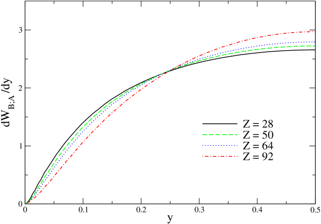
Figure 6: (Color online) The $2^{1}S_{0}$ two-photon energy distribution functions $dW_{B;A}/dy$, normalized to the corresponding total decay rates, plotted as a function of the reduced energy $y$ for He-like nickel, tin, europium, and uranium ions.

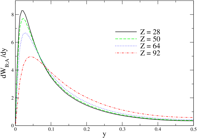
Figure 7: (Color online) The $2^{3}S_{1}$ two-photon energy distribution functions $dW_{B;A}/dy$, normalized to the corresponding total decay rates, plotted as a function of the reduced energy $y$ for He-like nickel, tin, europium, and uranium ions.

Since we employ the more accurate transition energy $\Delta^{(1)}_{AB}$ from Ref. Artemyev et al. (2005), our energy distribution function appears to be not exactly symmetric with respect to the center point at $y=0.5$. This asymmetry comes mainly due to the higher-order corrections included in the transition energy but neglected in the transition amplitude. In Tables 6, 7 and in Figs. 6, 7 we present the spectral-distribution functions $dW_{B;A}/dy$ calculated as a half-sum of the contributions at the points $y$ and $1-y$. For the $2^{1}S_{0}$ state the energy distribution function has one maximum at $y=0.5$, and in Table 6 we give also the reduced full width at half maximum (FWHM) values. The behavior of the reduced FWHM values as a function of $Z$ confirms those of Ref. Derevianko and Johnson (1997). For the $2^{3}S_{1}$ state the energy distribution function has two symmetric maxima in first and second half of the unit segment. In the center point (equal energy sharing) the distribution function is zero for the decay channels with the photons with the same multipole numbers (e.g., for the 2E1 decay). This is a consequence of the Bose-Einstein statistics, which forbids to construct a permutation symmetric two-photon state with total angular momentum $J_{\rm tot}=1$. Therefore, near the center point the distribution function is defined by the E1M2 channel, as it was noticed first in Ref. Dunford (2004). The value of $y$, where the first maximum is reached, is given in Table 7 together with the corresponding values of the reduced FWHM. In contrast to the results reported in Ref. Derevianko and Johnson (1997), we obtain a different energy distribution due to accounting for the higher multipoles contributions.

Table 6: The spectral distribution $dW_{B;A}/dy$ for the two-photon transition $2^{1}S_{0}\rightarrow 1^{1}S_{0}$ in He-like ions, in units s^-1. The reduced photon energy $y=k_{f_{1}}^{0}/\Delta^{(1)}_{AB}$ is the fraction of the total transition energy transported by one of the two photons. The reduced full widths at half maximum (FWHM) are also given. Numbers in brackets denote powers of ten.

$y$	$Z=28$	$Z=36$	$Z=41$	$Z=50$	$Z=64$	$Z=70$	$Z=80$	$Z=90$	$Z=92$
0.025	2.48[09]	1.09[10]	2.28[10]	6.78[10]	2.43[11]	3.79[11]	7.19[11]	1.24[12]	1.37[12]
0.050	5.16[09]	2.31[10]	4.92[10]	1.52[11]	5.77[11]	9.17[11]	1.78[12]	3.11[12]	3.44[12]
0.075	7.33[09]	3.32[10]	7.14[10]	2.24[11]	8.83[11]	1.43[12]	2.84[12]	5.05[12]	5.61[12]
0.100	9.10[09]	4.14[10]	8.97[10]	2.85[11]	1.15[12]	1.88[12]	3.80[12]	6.90[12]	7.68[12]
0.125	1.06[10]	4.82[10]	1.05[11]	3.36[11]	1.38[12]	2.27[12]	4.66[12]	8.58[12]	9.58[12]
0.150	1.18[10]	5.39[10]	1.17[11]	3.79[11]	1.57[12]	2.61[12]	5.42[12]	1.01[13]	1.13[13]
0.175	1.28[10]	5.86[10]	1.28[11]	4.16[11]	1.74[12]	2.90[12]	6.09[12]	1.15[13]	1.29[13]
0.200	1.36[10]	6.26[10]	1.37[11]	4.47[11]	1.89[12]	3.15[12]	6.67[12]	1.27[13]	1.42[13]
0.225	1.43[10]	6.60[10]	1.45[11]	4.73[11]	2.01[12]	3.37[12]	7.19[12]	1.37[13]	1.55[13]
0.250	1.49[10]	6.89[10]	1.51[11]	4.96[11]	2.12[12]	3.57[12]	7.64[12]	1.47[13]	1.66[13]
0.275	1.54[10]	7.13[10]	1.57[11]	5.15[11]	2.21[12]	3.73[12]	8.03[12]	1.55[13]	1.75[13]
0.300	1.58[10]	7.34[10]	1.61[11]	5.31[11]	2.29[12]	3.87[12]	8.37[12]	1.63[13]	1.84[13]
0.325	1.62[10]	7.51[10]	1.65[11]	5.45[11]	2.36[12]	4.00[12]	8.66[12]	1.69[13]	1.91[13]
0.350	1.65[10]	7.66[10]	1.68[11]	5.57[11]	2.42[12]	4.10[12]	8.90[12]	1.74[13]	1.97[13]
0.375	1.67[10]	7.77[10]	1.71[11]	5.66[11]	2.47[12]	4.18[12]	9.11[12]	1.79[13]	2.02[13]
0.400	1.69[10]	7.87[10]	1.73[11]	5.74[11]	2.50[12]	4.25[12]	9.27[12]	1.82[13]	2.07[13]
0.425	1.71[10]	7.94[10]	1.75[11]	5.79[11]	2.53[12]	4.30[12]	9.40[12]	1.85[13]	2.10[13]
0.450	1.72[10]	7.99[10]	1.76[11]	5.83[11]	2.55[12]	4.34[12]	9.49[12]	1.87[13]	2.12[13]
0.475	1.72[10]	8.02[10]	1.77[11]	5.86[11]	2.56[12]	4.36[12]	9.54[12]	1.88[13]	2.13[13]
0.500	1.73[10]	8.03[10]	1.77[11]	5.87[11]	2.57[12]	4.37[12]	9.56[12]	1.89[13]	2.14[13]
FWHM	0.814	0.809	0.804	0.793	0.771	0.761	0.743	0.722	0.718

Table 7: The spectral distribution $dW_{B;A}/dy$ for the two-photon transition $2^{3}S_{1}\rightarrow 1^{1}S_{0}$ in He-like ions, in units s^-1. The reduced photon energy $y=k_{f_{1}}^{0}/\Delta^{(1)}_{AB}$ is the fraction of the total transition energy transported by one of the two photons. The maximum point of the distribution $y_{\rm max}$ together with the reduced full widths at half maximum (FWHM) are also presented. Numbers in brackets denote powers of ten.

$y$	$Z=28$	$Z=36$	$Z=41$	$Z=50$	$Z=64$	$Z=70$	$Z=80$	$Z=90$	$Z=92$
0.010	1.68[06]	2.27[07]	8.13[07]	5.12[08]	4.22[09]	8.62[09]	2.40[10]	5.71[10]	6.70[10]
0.015	1.94[06]	2.59[07]	9.32[07]	6.02[08]	5.21[09]	1.09[10]	3.13[10]	7.63[10]	8.99[10]
0.020	1.99[06]	2.64[07]	9.56[07]	6.30[08]	5.68[09]	1.21[10]	3.57[10]	8.92[10]	1.05[11]
0.025	1.95[06]	2.58[07]	9.37[07]	6.26[08]	5.85[09]	1.26[10]	3.83[10]	9.75[10]	1.16[11]
0.030	1.87[06]	2.46[07]	8.98[07]	6.08[08]	5.83[09]	1.28[10]	3.95[10]	1.03[11]	1.22[11]
0.035	1.78[06]	2.33[07]	8.52[07]	5.83[08]	5.72[09]	1.27[10]	3.99[10]	1.05[11]	1.26[11]
0.040	1.68[06]	2.19[07]	8.04[07]	5.55[08]	5.55[09]	1.24[10]	3.97[10]	1.06[11]	1.27[11]
0.045	1.58[06]	2.06[07]	7.57[07]	5.26[08]	5.35[09]	1.21[10]	3.91[10]	1.06[11]	1.28[11]
0.050	1.48[06]	1.94[07]	7.12[07]	4.98[08]	5.14[09]	1.17[10]	3.83[10]	1.05[11]	1.27[11]
0.075	1.10[06]	1.43[07]	5.30[07]	3.78[08]	4.10[09]	9.54[09]	3.27[10]	9.42[10]	1.14[11]
0.100	8.40[05]	1.09[07]	4.05[07]	2.93[08]	3.27[09]	7.72[09]	2.72[10]	8.08[10]	9.87[10]
0.125	6.58[05]	8.53[06]	3.17[07]	2.31[08]	2.63[09]	6.28[09]	2.26[10]	6.85[10]	8.41[10]
0.150	5.25[05]	6.81[06]	2.54[07]	1.86[08]	2.14[09]	5.15[09]	1.88[10]	5.80[10]	7.15[10]
0.175	4.26[05]	5.52[06]	2.06[07]	1.51[08]	1.77[09]	4.27[09]	1.58[10]	4.93[10]	6.08[10]
0.200	3.50[05]	4.54[06]	1.69[07]	1.25[08]	1.47[09]	3.57[09]	1.33[10]	4.20[10]	5.20[10]
0.225	2.91[05]	3.76[06]	1.41[07]	1.04[08]	1.23[09]	3.01[09]	1.13[10]	3.60[10]	4.46[10]
0.250	2.43[05]	3.15[06]	1.18[07]	8.75[07]	1.04[09]	2.55[09]	9.63[09]	3.09[10]	3.84[10]
0.275	2.06[05]	2.66[06]	9.97[06]	7.42[07]	8.88[08]	2.18[09]	8.28[09]	2.68[10]	3.33[10]
0.300	1.75[05]	2.27[06]	8.51[06]	6.34[07]	7.63[08]	1.88[09]	7.16[09]	2.33[10]	2.90[10]
0.325	1.51[05]	1.96[06]	7.33[06]	5.47[07]	6.61[08]	1.63[09]	6.25[09]	2.04[10]	2.54[10]
0.350	1.31[05]	1.70[06]	6.38[06]	4.77[07]	5.79[08]	1.43[09]	5.50[09]	1.80[10]	2.25[10]
0.375	1.15[05]	1.50[06]	5.63[06]	4.22[07]	5.14[08]	1.27[09]	4.90[09]	1.61[10]	2.01[10]
0.400	1.03[05]	1.34[06]	5.05[06]	3.79[07]	4.62[08]	1.15[09]	4.43[09]	1.46[10]	1.83[10]
0.425	9.42[04]	1.23[06]	4.61[06]	3.47[07]	4.24[08]	1.05[09]	4.08[09]	1.35[10]	1.69[10]
0.450	8.80[04]	1.15[06]	4.31[06]	3.24[07]	3.97[08]	9.87[08]	3.83[09]	1.27[10]	1.59[10]
0.475	8.43[04]	1.10[06]	4.14[06]	3.11[07]	3.82[08]	9.49[08]	3.68[09]	1.22[10]	1.53[10]
0.500	8.31[04]	1.08[06]	4.08[06]	3.07[07]	3.77[08]	9.36[08]	3.64[09]	1.21[10]	1.51[10]
$y_{\rm max}$	0.020	0.019	0.020	0.019	0.024	0.030	0.035	0.041	0.043
FWHM	0.079	0.077	0.079	0.087	0.106	0.116	0.134	0.154	0.158

IV Summary

In summary, we have presented a systematic quantum electrodynamic description for the first-order interelectronic-interaction corrections to the two-photon transition probabilities in He-like ions. A local screening potential has been included in the zeroth-order approximation in the framework of an extended Furry representation, and the corresponding expressions for the counterterms have been derived. Such a treatment of the electron-correlation effects allows us to control the gauge-invariance of each term in the perturbation expansion and to estimate an uncertainty due to the truncation of this expansion. The total two-photon decay rates and the spectral distribution functions have been evaluated for the transitions $2^{1}S_{0}\rightarrow 1^{1}S_{0}$ and $2^{3}S_{1}\rightarrow 1^{1}S_{0}$ in the He-like ions with nuclear charges in the range $28\leq Z\leq 92$. The results of the calculations performed have been compared with previous calculations and with experimental data. The present calculations of the two-photon decays of the $2^{1}S_{0}$ and $2^{3}S_{1}$ states in He-like ions can be utilized for studying the parity non-conservation phenomena in He-like ions Schäfer et al. (1989); Labzowsky et al. (2001); Shabaev et al. (2010) as well as for investigations of the contributions of higher multipoles to the energy distribution.

References

Göppert-Mayer (1931)
M. Göppert-Mayer,
Ann. Phys. 9,
273 (1931).
Drake (1986)
G. W. F. Drake,
Phys. Rev. A 34,
2871 (1986).
Santos et al. (1998)
J. P. Santos,
F. Parente, and
P. Indelicato,
Eur. Phys. J. D 3,
43 (1998).
Surzhykov et al. (2005)
A. Surzhykov,
P. Koval, and
S. Fritzsche,
Phys. Rev. A 71,
022509 (2005).
Labzowsky et al. (2005)
L. N. Labzowsky,
A. V. Shonin,
and D. A.
Solovyev, J. Phys. B
38, 265 (2005).
Amaro et al. (2009)
P. Amaro,
J. P. Santos,
F. Parente,
A. Surzhykov,
and
P. Indelicato,
Phys. Rev. A 79,
062504 (2009).
Dalgarno (1966)
A. Dalgarno,
Mon. Not. R. Astron. Soc. 131,
311 (1966).
Bely and Faucher (1969)
O. Bely and
P. Faucher,
Astron. Astrophys. 1,
37 (1969).
Drake et al. (1969)
G. W. F. Drake,
G. A. Victor,
and A. Dalgarno,
Phys. Rev. 180,
25 (1969).
Derevianko and Johnson (1997)
A. Derevianko and
W. R. Johnson,
Phys. Rev. A 56,
1288 (1997).
Surzhykov et al. (2010)
A. Surzhykov,
A. Volotka,
F. Fratini,
J. P. Santos,
P. Indelicato,
G. Plunien,
Th. Stöhlker, and
S. Fritzsche,
Phys. Rev. A 81,
042510 (2010).
Marrus et al. (1986)
R. Marrus,
V. San Vicente,
P. Charles,
J. P. Briand,
F. Bosch,
D. Liesen, and
I. Varga,
Phys. Rev. Lett. 56,
1683 (1986).
Dunford
et al. (1993a)
R. W. Dunford,
H. G. Berry,
S. Cheng,
E. P. Kanter,
C. Kurtz,
B. J. Zabransky,
A. E. Livingston,
and L. J.
Curtis, Phys. Rev. A
48, 1929
(1993a).
Dunford
et al. (1993b)
R. W. Dunford,
H. G. Berry,
D. A. Church,
M. Hass,
C. J. Liu,
M. L. A. Raphaelian,
B. J. Zabransky,
L. J. Curtis,
and A. E.
Livingston, Phys. Rev. A
48, 2729
(1993b).
Mokler et al. (1990)
P. H. Mokler,
S. Reusch,
A. Warczak,
Z. Stachura,
T. Kambara,
A. Müller,
R. Schuch, and
M. Schulz,
Phys. Rev. Lett. 65,
3108 (1990).
Ali et al. (1997)
R. Ali,
I. Ahmad,
R. W. Dunford,
D. S. Gemmell,
M. Jung,
E. P. Kanter,
P. H. Mokler,
H. G. Berry,
A. E. Livingston,
S. Cheng,
et al., Phys. Rev. A
55, 994 (1997).
Schäffer et al. (1999)
H. W. Schäffer,
P. H. Mokler,
R. W. Dunford,
C. Kozhuharov,
A. Krämer,
A. E. Livingston,
T. Ludziejewski,
H.-T. Prinz,
P. Rymuza,
L. Sarkadi,
et al., Phys. Lett. A
260, 489 (1999).
Kumar et al. (2009)
A. Kumar,
S. Trotsenko,
A. V. Volotka,
D. Banaś,
H. F. Beyer,
H. Bräuning,
A. Gumberidze,
S. Hagmann,
S. Hess,
C. Kozhuharov,
et al., Eur. Phys. J. Special Topics
169, 19 (2009).
Trotsenko et al. (2010)
S. Trotsenko,
A. Kumar,
A. V. Volotka,
D. Banaś,
H. F. Beyer,
H. Bräuning,
S. Fritzsche,
A. Gumberidze,
S. Hagmann,
S. Hess, et al.,
Phys. Rev. Lett. 104,
033001 (2010).
Savukov and Johnson (2002)
I. M. Savukov and
W. R. Johnson,
Phys. Rev. A 66,
062507 (2002).
Shabaev et al. (2010)
V. M. Shabaev,
A. V. Volotka,
C. Kozhuharov,
G. Plunien, and
Th. Stöhlker, Phys.
Rev. A 81, 052102
(2010).
Lapierre et al. (2005)
A. Lapierre,
U. D. Jentschura,
J. R.
Crespo López-Urrutia,
J. Braun,
G. Brenner,
H. Bruhns,
D. Fischer,
A. J. González Martínez,
Z. Harman,
W. R. Johnson,
et al., Phys. Rev. Lett.
95, 183001
(2005).
Lapierre et al. (2006)
A. Lapierre,
J. R.
Crespo López-Urrutia,
J. Braun,
G. Brenner,
H. Bruhns,
D. Fischer,
A. J. González Martínez,
V. Mironov,
C. Osborne,
G. Sikler,
et al., Phys. Rev. A
73, 052507
(2006).
Tupitsyn et al. (2005)
I. I. Tupitsyn,
A. V. Volotka,
D. A. Glazov,
V. M. Shabaev,
G. Plunien,
J. R.
Crespo López-Urrutia,
A. Lapierre, and
J. Ullrich,
Phys. Rev. A 72,
062503 (2005).
Volotka et al. (2006)
A. V. Volotka,
D. A. Glazov,
G. Plunien,
V. M. Shabaev,
and I. I.
Tupitsyn, Eur. Phys. J. D
38, 293 (2006).
Volotka
et al. (2008a)
A. V. Volotka,
D. A. Glazov,
G. Plunien,
V. M. Shabaev,
and I. I.
Tupitsyn, Eur. Phys. J. D
48, 167
(2008a).
Indelicato et al. (2004)
P. Indelicato,
V. M. Shabaev,
and A. V.
Volotka, Phys. Rev. A
69, 062506
(2004).
V. M. Shabaev, Izv. Vuz. Fiz. 33, 43
[Sov. Phys. J. 33, 660 (1990)].() (1990)V. M. Shabaev, Izv. Vuz. Fiz. 33, 43
(1990) [Sov. Phys. J. 33, 660 (1990)].
V. M. Shabaev, Teor. Mat. Fiz. 82, 83
[Theor. Math. Phys. 82, 57 (1990)].() (1990)V. M. Shabaev, Teor. Mat. Fiz. 82, 83
(1990) [Theor. Math. Phys. 82, 57 (1990)].
Shabaev (2002)
V. M. Shabaev,
Phys. Rep. 356,
119 (2002).
O. Yu. Andreev
et al. (2009)
O. Yu. Andreev,
L. N. Labzowsky,
and G. Plunien,
Phys. Rev. A 79,
032515 (2009).
O. Yu. Andreev
et al. (2008)
O. Yu. Andreev,
L. N. Labzowsky,
G. Plunien, and
D. A. Solovyev,
Phys. Rep. 455,
135 (2008).
Berestetsky et al. (1982)
V. B. Berestetsky,
E. M. Lifshitz,
and L. P.
Pitaevsky, Quantum Electrodynamics
(Pergamon Press, Oxford, 1982).
Itzykson and Zuber (1980)
C. Itzykson and
J.-B. Zuber,
Quantum Field Theory
(McGraw-Hill, New York, 1980).
Labzowsky et al. (2009)
L. Labzowsky,
D. Solovyev, and
G. Plunien,
Phys. Rev. A 80,
062514 (2009).
Labzowsky and Shonin (2004)
L. N. Labzowsky
and A. V.
Shonin, Phys. Rev. A
69, 012503
(2004).
Glazov et al. (2006)
D. A. Glazov,
A. V. Volotka,
V. M. Shabaev,
I. I. Tupitsyn,
and G. Plunien,
Phys. Lett. A 357,
330 (2006).
Volotka
et al. (2008b)
A. V. Volotka,
D. A. Glazov,
I. I. Tupitsyn,
N. S. Oreshkina,
G. Plunien, and
V. M. Shabaev,
Phys. Rev. A 78,
062507 (2008b).
Shabaev et al. (2004)
V. M. Shabaev,
I. I. Tupitsyn,
V. A. Yerokhin,
G. Plunien, and
G. Soff,
Phys. Rev. Lett. 93,
130405 (2004).
Angeli (2004)
I. Angeli, At.
Data Nucl. Data Tables 87, 185
(2004).
Kozhedub et al. (2008)
Y. S. Kozhedub,
O. V. Andreev,
V. M. Shabaev,
I. I. Tupitsyn,
C. Brandau,
C. Kozhuharov,
G. Plunien, and
T. Stöhlker,
Phys. Rev. A 77,
032501 (2008).
Artemyev et al. (2005)
A. N. Artemyev,
V. M. Shabaev,
V. A. Yerokhin,
G. Plunien, and
G. Soff,
Phys. Rev. A 71,
062104 (2005).
Dunford (2004)
R. W. Dunford,
Phys. Rev. A 69,
062502 (2004).
Simionovici et al. (1993)
A. Simionovici,
B. B. Birkett,
J. P. Briand,
P. Charles,
D. D. Dietrich,
K. Finlayson,
P. Indelicato,
D. Liesen, and
R. Marrus,
Phys. Rev. A 48,
1695 (1993).
Schäfer et al. (1989)
A. Schäfer,
G. Soff,
P. Indelicato,
B. Müller, and
W. Greiner,
Phys. Rev. A 40,
7362 (1989).
Labzowsky et al. (2001)
L. N. Labzowsky,
A. V. Nefiodov,
G. Plunien,
G. Soff,
R. Marrus, and
D. Liesen,
Phys. Rev. A 63,
054105 (2001).