Statefinder analysis of the superfluid Chaplygin gas model

Abstract

The statefinder indices are employed to test the superfluid Chaplygin gas (SCG) model describing the dark sector of the universe. The model involves Bose-Einstein condensate (BEC) as dark energy (DE) and an excited state above it as dark matter (DM). The condensate is assumed to have a negative pressure and is embodied as an exotic fluid with the Chaplygin equation of state. Excitations forms the normal component of superfluid. The statefinder diagrams show the discrimination between the SCG scenario and other models with the Chaplygin gas and indicates a pronounced effect of the DM equation of state and an indirect interaction between their two components on statefinder trajectories and a current statefinder location.

Department of General Relativity and Gravitation,
Kazan Federal University,
Kremlyovskaya st. 18, Kazan 420008, Russia

Email address: vladipopov@mail.ru

Keywords: accelerated expansion, Dark Energy, Dark Matter, relativistic superfluid, Chaplygin gas, statefinder

PACS: 95.36.+x, 95.35.+d, 98.80.-k, 98.80.Jk, 47.37.+q

1 Introduction

The energy content of the Universe is a fundamental issue in cosmology. Observational data, such as Type Ia Supernovae (SNIa) [1], Cosmic Microwave Background (CMB) [2] and Large Scale Structure [3], are evidence of accelerating flat Friedmann-Robertson-Walker model, constituted of about 1/3 of baryonic and dark matter and about 2/3 of a dark energy component.

The essential feature of DE is that its pressure must be negative to reproduce the present accelerated cosmic expansion. There are a few candidates for DE incorporated in competing cosmological scenarios. The simplest DE model, the cosmological constant, is indeed the vacuum energy with the equation of state $p=-\rho$. A number of models, such as quintessence [4], k-essence [5], phantom [6] and etc., are based on scalar field theories. Braneworld models explain the acceleration through the five-dimensional general relativity [7]. The Chaplygin gas model, also denoted as quartessence, exploits a negative pressure fluid, which is inversely proportional to the energy density [8]. For a more detail review of DE models and references see [9]. Besides, there are models unifying DE and DM, including a some kind of scalar fields [10], generalized Chaplygin gas (GCG) [11, 12] and superfluid Chaplygin gas (SCG) [13].

In order to differentiate these various DE models, Sahni et al. [14] introduce a new geometrical diagnostic pair $\{r,s\}$, called statefinder, which involves the third order derivative of the scale factor with respect to time. Its important attribute is that the spatially flat $\Lambda$CDM has a fixed point $\{r,s\}=\{1,0\}$. Departure of a DE model from this fixed point is a good way of establishing the ‘distance’ of this model from flat $\Lambda$CDM. The statefinder diagnostic has been also applied to several DE models [15, 16, 17, 18, 19, 20] to differentiate them from $\Lambda$CDM and one from other. In addition the values of the statefinder pair can be extracted from data of SuperNova Acceleration Probe (SNAP) type experiments [14, 15] to obtain constraints on the models.

In this letter the statefinder diagnostic is applied to the SCG model developed in [13]. It represents the dark sector of the universe as a superfluid where the superfluid condensate is considered as DE and the normal component is interpreted as DM. The model is based on the action

$$S=\int\left(-\frac{R}{16\pi G}+{\cal L}\right)\sqrt{-g}\,{\rm{d}}^{4}x\,,$$ (1)

where Lagrangian ${\cal L}$ associated with a generalized hydrodynamic pressure function depends only on one variable if we consider pure condensate, and on three variables when we include the excitation gas. To provide the accelerated expansion the negative pressure of the superfluid background obeys Chaplygin’s equation of state. In Sec. 2 and 3 the SCG model is briefly outlined. The statefinder evolution and differentiation between SCG model and another models with the Chaplygin gas are discussed in Sec. 4. The metric signature $(+---)$ is adopted in this work.

2 Relativistic superfluid dynamics

An efficient approach to description of the excited state is two-fluid hydrodynamics. This theory does not depend on details of microscopic structure of the quantum liquid and exploits effective macroscopic quantities. In the theory there exist two independent flows, the coherent motion of the ground state named a superfluid component, and a normal component produced by the quasiparticle gas. For this reason it is necessary to increase the number of independent variables in the generalized pressure (8) from one to three [21]. They correspond to three scalar invariants which can be constructed from the pair of independent vectors, namely superfluid $\mu_{\alpha}$ and thermal $\theta_{\alpha}$ momentum covectors so that the general variation of the generalized pressure in a fixed background is

$$\delta P=\delta{\cal L}=n^{\alpha}\delta\mu_{\alpha}+s^{\alpha}\delta\theta_{\alpha}\,.$$ (2)

The coefficients $n^{\alpha}$ and $s^{\alpha}$ are to be interpreted as particle number and entropy currents correspondingly. By virtue of its invariance the pressure is given as a function of three independent variables, $I_{1}=\frac{1}{2}\mu_{\alpha}\mu^{\alpha},\,I_{2}=\mu_{\alpha}\theta^{\alpha},\,I_{3}=\frac{1}{2}\theta_{\alpha}\theta^{\alpha}$. Taking the derivatives of the pressure, one finds

$$n^{\alpha}=\frac{\partial P}{\partial I_{1}}\mu^{\alpha}+\frac{\partial P}{\partial I_{2}}\theta^{\alpha},\qquad s^{\alpha}=\frac{\partial P}{\partial I_{2}}\mu^{\alpha}+\frac{\partial P}{\partial I_{3}}\theta^{\alpha}.$$ (3)

As soon as the generalized pressure is the Lagrangian density in the action (1) its variation with respect to the metric gives the energy-momentum tensor

$$T_{\alpha\beta}=\frac{\partial P}{\partial I_{1}}\mu_{\alpha}\mu_{\beta}+\frac{\partial P}{\partial I_{2}}(\mu_{\alpha}\theta_{\beta}+\theta_{\alpha}\mu_{\beta})+\frac{\partial P}{\partial I_{3}}\theta_{\alpha}\theta_{\beta}-Pg_{\alpha\beta}\,.$$ (4)

Instead of the thermal momentum $\theta_{\alpha}$ let us introduce an inverse temperature vector $\beta^{\alpha}=s^{\alpha}/(s^{\beta}\theta_{\beta})$ which one uses as the independent vector together with the superfluid momentum $\mu_{\alpha}$ since they are comoving to the excitation gas and the condensate respectively. Corresponding unit 4-velocities are

$$U^{\alpha}=\frac{\beta^{\alpha}}{\sqrt{\beta^{\beta}\beta_{\beta}}}\,,\qquad V^{\alpha}=\frac{\mu^{\alpha}}{\sqrt{\mu^{\beta}\mu_{\beta}}}\,.$$ (5)

In place of the scalars $I_{1},\ I_{2},\ I_{3}$ one uses new three invariants, a chemical potential $\mu=\sqrt{\mu^{\beta}\mu_{\beta}}$, scalar $\gamma=V_{\alpha}U^{\alpha}$ associated with the relative motion of the components, and inverse temperature with respect to the reference frame comoving to the normal component $\beta=\sqrt{\beta^{\beta}\beta_{\beta}}\,$.

Using (3) and (5) the energy-momentum tensor and the particle number current are readily represented as

$$n^{\alpha} = n_{\rm c}V^{\alpha}+n_{\rm n}U^{\alpha},$$ (6)

$$T_{\alpha\beta} = \mu n_{\rm c}V_{\alpha}V_{\beta}+W_{\rm n}U_{\alpha}U_{\beta}-Pg_{\alpha\beta}\,.$$ (7)

The ground state is described by the generalized hydrodynamic pressure function depending only on $\mu$. We will consider the condensate with the function of the generalized pressure in the form

$$P(\mu)=p_{\rm c}=-\sqrt{A-\lambda\mu^{2}}\,.$$ (8)

It leads to the following particle and energy densities

$$n_{\rm c}=\frac{\lambda\mu}{\sqrt{A-\lambda\mu^{2}}}\,,\qquad\rho_{\rm c}=\frac{A}{\sqrt{A-\lambda\mu^{2}}}\,.$$ (9)

It is easy to see that if to eliminate the chemical potential $\mu$ one can obtain

$$n_{\rm c}=\sqrt{\frac{\lambda}{A}}\sqrt{\rho_{\rm c}^{2}-A}\,,\qquad p_{\rm c}=-\frac{A}{\rho_{\rm c}}\,,\qquad$$ (10)

and the adiabatic speed of sound

$$c_{\rm s}^{2}=\frac{\,{\rm{d}}p_{\rm c}}{\,{\rm{d}}\rho_{\rm c}}=\frac{A}{\rho_{\rm c}^{2}}\,.$$ (11)

The equation of state (10) is uniquely proper to the Chaplygin gas suggested by Kamenshchik et al. [8] as an alternative to quintessence and developed by a number of authors for description of the dark sector of the universe [11]. In contrast to these works where pressure of the Chaplygin gas is formed by both DE and DM, this model implies that the equation of state (10) concerns with only BEC which is interpreted as DE. Note that the generalized pressure (8) can be obtained from the Lagrangian

$${\cal L}=\partial_{\nu}\phi^{*}\partial^{\nu}\phi-M\left(\frac{\phi^{*}\phi}{\lambda}+\frac{\lambda}{\phi^{*}\phi}\right)$$ (12)

for a complex scalar field $\phi$ in the WKB-approximation [13].

The interesting aspect of the pressure function (8) is that it is a hydrodynamical representation of the generalized Born-Infeld Lagrangian

$${\cal L}_{\text{BI}}=-\sqrt{A}\sqrt{1-\partial_{\nu}\theta\,\partial^{\nu}\theta}$$ (13)

describing a (3+1)-dimensional brane universe with the scalar field $\theta$ in a (4+1)-dimensional bulk [11].

More detail information about the excited state can be derived from statistical description of the elementary excitations. The quasiparticle energy spectrum has a significant nonlinear dispersion at high energy, and therefore completely relativistic description has been carried out only for a low energy excitations, phonons [22, 23]. Based on the relativistic kinetic theory of the phonon gas [23] one in particular can obtain

$$\frac{\mu n_{\rm n}}{\gamma}=(1-c_{\text{s}}^{2})W_{\rm n}$$ (14)

when phonons prevail over another sorts of quasiparticles.

Let us assume that the generalized pressure function is separated as follows:

$$P(\mu,\beta,\gamma)=p_{\textrm{c}}(\mu)+p_{\textrm{n}}(\mu,\beta,\gamma)$$ (15)

and

$$p_{\textrm{n}}(\mu,\beta,\gamma)=\frac{B(\mu)}{\beta^{\nu+1}\left(1-\gamma^{2}\left(1-c_{\text{s}}^{2}\right)\right)^{(\nu+1)/2}}$$ (16)

that is inspired by the equilibrium pressure for the phonon gas [22] corresponding to $\nu=3$. Eq. (16) leads to the barotropic equation of state

$$p_{\rm n}=\frac{1-\gamma^{2}\left(1-c_{\text{s}}^{2}\right)}{\nu+1}W_{\rm n}\,.$$ (17)

Moreover, the ansatz (15) and (16) proves to be convenient for a number of reasons. The equation of state (16) makes possible to avoid a detail consideration of the full quasiparticle spectrum. Manipulating the sole parameter $\nu$ one can simulate a behavior of the normal component as DM. It also simplifies the following study of the cosmic evolution. This ansatz keeps the condensate self-dependent, i.e. eqs. (10) and (11) remain valid for the condensate in the framework of two-fluid dynamics and allow to naturally divide the total energy density into DE and DM fractions.

We restrict our consideration to the equation of state (17) for the normal component situated between the dust one and the stiff one. It is evident from eq. (17) that this constraint implies $\nu\geq 1$.

3 Universe with SCG

The cosmic medium is now regarded as a matter which particularly is in the BEC state and its particle number current and energy-momentum tensor have the form (6) and (7) where the superfluid background obeys the equation of state (10) and the excited state is described by the relations (14) and (17).

Let us consider a homogeneous and isotropic spatially flat universe. In this case the superfluid and normal velocities are equal and thus $\gamma=1$. Einstein’s equations then reduce to

$$3\frac{\dot{a}^{2}}{a^{2}}=8\pi G\rho_{\textrm{tot}}\,,\qquad-6\frac{\ddot{a}}{a}=8\pi G(3p_{\textrm{tot}}+\rho_{\textrm{tot}})\,,$$ (18)

where $\rho_{\textrm{tot}}$ consists of the condensate density $\rho_{\textrm{c}}$ and the normal one $\rho_{\textrm{n}}=W_{\textrm{n}}-p_{\textrm{n}}$ that are interpretable as DE and DM densities respectively, and $p_{\textrm{tot}}=p_{\textrm{c}}+p_{\textrm{n}}=P$. In accordance with the integrability conditions of the Einstein equations we require local energy-momentum conservation $\nabla_{\mu}T^{\mu\nu}=0$ that yields

$$\dot{\rho}_{\textrm{tot}}+3\frac{\dot{a}}{a}(p_{\textrm{tot}}+\rho_{\textrm{tot}})=0\,.$$ (19)

The interaction between DE and DM is implicitly included in equation (19) and also in particle number conservation $\nabla_{\mu}n^{\mu}=0$ that leads to

$$\dot{n}_{\textrm{tot}}+3\frac{\dot{a}}{a}n_{\textrm{tot}}=0\quad\Longrightarrow\quad n_{\textrm{c}}+n_{\textrm{n}}=\frac{n_{0}}{a^{3}}\,,\ n_{0}=\mbox{const}.$$ (20)

Taking into account the expressions (14), (17) with $\gamma=1$ and (20), eqs. (18) and (19) are reduced to following two dimensionless equations:

$$3(1+\nu)\frac{\dot{a}^{2}}{a^{2}}=\frac{1}{\rho_{\text{c}}}+\frac{k}{a^{3}}\left(\frac{\nu\rho_{\text{c}}}{\sqrt{\rho_{\text{c}}^{2}-1}}+\frac{\sqrt{\rho_{\text{c}}^{2}-1}}{\rho_{\text{c}}}\right),$$ (21)

$$3\frac{\dot{a}}{a}\left(1+\nu-\frac{k}{a^{3}}\frac{1}{\sqrt{\rho_{\text{c}}^{2}-1}}\right)+\frac{\dot{\rho}_{\text{c}}}{\rho_{\text{c}}}\left(1-\frac{k}{a^{3}}\left(\frac{1}{\sqrt{\rho_{\text{c}}^{2}-1}}-\frac{\nu\rho_{\text{c}}^{2}}{(\rho_{\text{c}}^{2}-1)^{3/2}}\right)\right)=0\,,$$ (22)

where the notation $\rho_{\text{c}}$ is used now for the dimensionless energy density $\rho_{\text{c}}/\sqrt{A}$ as well as $\rho_{\text{n}}$ will be used for $\rho_{\text{n}}/\sqrt{A}$ and etc. The dimensionless time variable $t^{\prime}$ is connected with real time $t$ as $t^{\prime}=\sqrt{8\pi GA^{1/2}}\,t$ and $k=n_{0}/\sqrt{\lambda}$.

In the formal limit $\nu\to\infty$ eqs. (21) and (22) are solved analytically. As obvious from (17) the quasiparticle pressure is neglected and DM behaves as dust-like matter. In this case eq. (22) yields the condensate energy density in the form

$$\rho_{\rm c}=\sqrt{\frac{k^{2}}{(a^{3}+\kappa_{0})^{2}}+1}\,,$$ (23)

and the DM energy density is governed by the law

$$\rho_{\textrm{n}}=\frac{\kappa_{0}}{a^{3}}\sqrt{\frac{k^{2}}{(a^{3}+\kappa_{0})^{2}}+1}\,.$$ (24)

It is clear from (23) and (24) the integration constant $\kappa_{0}$ is the current ratio between the DM and DE energy densities.

At the beginning stage (i.e. for small $a$) the total energy density is approximated by $\rho_{\textrm{tot}}\propto a^{-3}$ that corresponds to a universe dominated by dust-like matter. The same behavior is a feature of the Chaplygin gas [8] but even though in this model the condensate has the same equation of state, such dependence is due to the normal component.

At the late stage (i.e. for large $a$) $\rho_{\textrm{tot}}\to 1$. Separating now DE and DM contributions one finds the subleading terms are

$$\rho_{\rm c}\sim 1+\frac{k^{2}}{2}a^{-6},\qquad\rho_{\textrm{n}}\sim\frac{\kappa_{0}}{a^{3}}\,,$$ (25)

whereas the scale factor time evolution corresponds to de Sitter spacetime, namely, $a\propto e^{t^{\prime}/\sqrt{3}}$.

Figure 1: The ratio of the energy density to the critical density for both components of SCG as a function of the redshift $z$ for $k=.2$ and the current value of $\rho_{\text{c}}(t_{0})=1.01$. The quantity $\nu$ varies as 1 (dot-dashed line), 5 (dashed line) and 25 (solid line).

When $\nu$ has a finite value the asymptotic behavior of $\rho_{\text{c}}$ is the same as it is found in the case with pressureless DM while $\rho_{\text{n}}\propto a^{-3(1-1/\nu)}$ for small $a$, and $\rho_{\text{n}}\propto a^{-3(1+1/\nu)}$ for large $a$. As before the universe falls within de Sitter phase in the far future. At the intermediate stage eqs. (21) and (22) are solved numerically. The figure 1 depicts an evolution of the normalized energy densities $\Omega_{\rm c}$ and $\Omega_{\rm n}$ of DE and DM respectively. The curves are plotted for different values of $\nu$ and fixed $k$ and the current value of $\rho_{\text{c}}$. The latter is close to 1 to provide the correspondence with the current observational value of the DE fraction $\Omega_{\rm c}\approx 0.7$.

Photometric observations of apparent Type Ia supernovae attests that the recent cosmological acceleration commenced at $0.3<z_{\text{T}}<1$ [24]. To satisfy this condition the quantity $\nu$ have to be large, $\nu\geq 20$. This implies a lower effective sound speed for the normal component evolving as $c_{\text{s}}/\sqrt{\nu}$. In this case properties of the normal component are close to CDM. Note, that in superfluid helium a lower second sound speed is provided by quasiparticles from the nonlinear part of the energy spectrum (such as rotons). To develop more realistic model, a wide quasiparticle spectrum should be taken into account. In the context of the pure phonon consideration they are not taken into account and their influence is simulated with a large value of $\nu$.

4 Statefinder diagnostic

In this section we focus our attention to the statefinder diagnostic of the SCG model. The parameter pair $\{r,s\}$ called ”statefinder” was introduced by Sahni et al. [14] for the purpose to differentiate between competing cosmological scenarios involving DE. The statefinder test is a geometrical one based on the expansion of the scale factor $a(t)$ near the present time $t_{0}$:

$$a(t)=1+H_{0}(t-t_{0})-\frac{1}{2}q_{0}H_{0}^{2}(t-t_{0})^{2}+\frac{1}{6}r_{0}H_{0}^{3}(t-t_{0})^{3}+\ldots\,,$$ (26)

where $a(t_{0})=1$ and $H_{0},\ q_{0},\ r_{0}$ are the current values of the Habble constant $H=\dot{a}/a$, deceleration factor $q=-\ddot{a}/aH^{2}$ and the former statefinder index $r=\dddot{a}/aH^{3}$ respectively. The latter index $s$ is the combination of $r$ and $q$: $s=(r-1)/3(q-1/2)$.

Since the different cosmological models exhibit qualitatively different trajectories in the $r-s$, $q-r$ or $q-s$ planes, the statefinder diagnostic is a good tool to distinguish them. The remarkable property of the pair $\{r,s\}$ is that the $\Lambda$CDM corresponds to the fixed point $\{r,s\}=\{1,0\}$.

In fact, the statefinder diagnostic has been successfully used to test a number of models such as the cosmological constant, the quintessence [15], the phantom [16], the Chaplygin gas [17, 15], the holographic dark energy models [18], the interacting dark energy models [19] and etc. [20]. On the other hand the statefinder indices can be estimated from SNAP type experiment [14, 15] to examine DE models from the observational data. In what follows we will calculate the statefinder parameters for the SCG model and plot the evolution trajectories in the statefinder planes.

The deceleration factor and the statefinder pair can also be expressed as

$$q = \frac{1}{2}\left(1+3\frac{p_{\text{tot}}}{\rho_{\text{tot}}}\right),$$ (27)

$$r = 1+\frac{9(\rho_{\text{tot}}+p_{\text{tot}})}{2\rho_{\text{tot}}}\,\frac{\dot{p}_{\text{tot}}}{\dot{\rho}_{\text{tot}}}\,,$$ (28)

$$s = \frac{(\rho_{\text{tot}}+p_{\text{tot}})}{p_{\text{tot}}}\,\frac{\dot{p}_{\text{tot}}}{\dot{\rho}_{\text{tot}}}\,,$$ (29)

where the overdot denotes the the derivative with respect to the time. Using the dimensionless energy density and pressure expressions (28) and (29) can rewritten as

$$r = 1-\frac{3\sqrt{3}}{2}\,\frac{\dot{p}_{\text{tot}}}{\rho_{\text{tot}}^{3/2}}\,,$$ (30)

$$s = -\frac{\dot{p}_{\text{tot}}}{p_{\text{tot}}\sqrt{3\rho_{\text{tot}}}}\,,$$ (31)

where the overdot denotes now the the derivative with respect to the dimensionless time.

It is because the SCG model uses the unified conservation laws for DM and DE and the DM pressure is non-zero in general, that the expressions (30) and (31) are best suited to calculate the statefinder indices to analyze the impact of the SCG parameters on the statefinder location and reveal the difference in the statefinder evolution for some models with the Chaplygin gas.

First we consider the special case $\nu\to\infty$ when the normal component is pressureless and the DE and DM energy densities evolve according to the expressions (23) and (24) respectively. In this case one can obtain explicit dependance $r(s)$ but in view of it complexity it is expressed as follows

$$q = \frac{1}{2}\left(1-\frac{3a^{3}\left(a^{3}+\kappa_{0}\right)}{k^{2}+\left(a^{3}+\kappa_{0}\right)^{2}}\right),$$ (32)

$$r = 1+\frac{9}{2}\,\frac{k^{2}a^{6}}{\left(k^{2}+\left(a^{3}+\kappa_{0}\right)^{2}\right)^{2}}\,,$$ (33)

$$s = -\frac{k^{2}a^{3}}{\left(a^{3}+\kappa_{0}\right)^{2}\left(k^{2}+\left(a^{3}+\kappa_{0}\right)^{2}\right)}\,,$$ (34)

where the scale factor $a$ appears as a natural parameter.

The value of $k$ is directly related to the scale factor corresponding to the transition from the deceleration to the acceleration. It is agreed that the transition occurs at $0.3<z_{\text{T}}<1$ [24] resulting in the restriction $k<0.652$ for dust-like normal component.

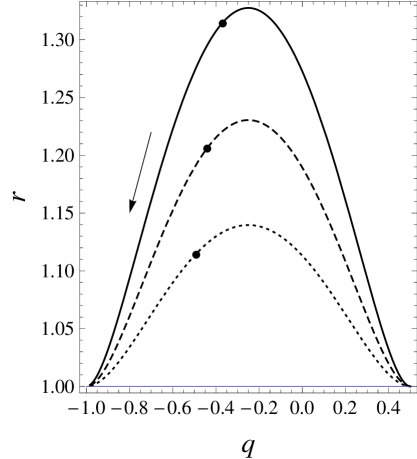
Figure 2: The statefinder evolution diagrams for the SCG model with the dust-like normal component. The quantity $k$ varies as 0.653 (solid line), 0.488 (dashed line) and 0.345 (dotted line). Dots mark the current values of the statefinder parameters and arrows show the evolution direction of the statefinder trajectories. The star denotes the $\Lambda$CDM location.

In the figure 2 we plot the evolution trajectories in the $s-r$ and $q-r$ planes assuming the current DE fraction $\Omega_{\Lambda 0}=0.7$ and varying $k$ as 0.652, 0.488 and 0.345 that corresponds to $z_{\text{T}}=$0.3, 0.4 and 0.5 respectively.

The trajectory in the $s-r$ plane begins and ends at the same point corresponding to the $\Lambda$CDM. This is the feature of the SCG model with the pressureless DM component. It does not take into account the radiation and therefore the total pressure is the negative DE pressure and $q<1/2$ through all the universe evolution. The value $k=0$ corresponds to the transition redshift of $\Lambda$CDM scenario $z_{\text{T}}=(\kappa_{0}/2)^{-1/3}-1\approx 0.671$. In this case the loop in the figure 2 degenerates into the fixed point {0,1} and the SCG model coincides with $\Lambda$CDM.

When $\nu$ is finite the pressure of DM is positive and the expressions (30) and (31) are directly used to calculate the statefinder evolution based on the numerical solution of eqs. (21) and (22). In the figure 3 we plot the evolution trajectories $r(s)$ and $r(q)$ for the various values of the quantity $\nu$.

At early times the DM pressure and energy density exceed the DE ones and ensure that the total pressure is positive. At the present stage of DE dominance the universe expands with acceleration driven by the negative total pressure. Between these regimes there is a moment of time when the negative pressure of DE is balanced by the positive pressure of DM. In this point the total pressure is zero and $s\to\infty$. In fact, this point exists in the universe evolution even though DM is pressureless when we take into account the whole energy content of the universe. Moreover the most considerable contribution in the positive pressure at this stage is given by the radiation. The non-zero DM pressure only shifts the moment of time when $p_{\text{tot}}=0$. Trajectories in the figure 3 are shown after this moment to focus the attention to the problem of the recent accelerated expansion of the universe.

Another quantity in the SCG model, $k$, realizes the indirect interaction between two components. It is clear from eqs. (21) and (22) that varying $k$ can be counterbalanced by rescaling of the scale factor $a$ leaving the equations invariant. However, for a fixed ratio between the DM and DE energy densities different $k$ are corresponded to different trajectories. Although the equations can be solved for any $k$, it is restricted by the observational estimations of the transition redshift $z_{\text{T}}$ [24]. For the current DE content $\Omega_{\Lambda 0}=0.7$ the value of $k$ does not exceed 0.652 determined by the limiting case of the pressureless normal component. The figure 3 depicts the evolution curves for $k=0.2$ and varying $k$ gives the similar plots which are different only in a quantitative sense.

Figure 3: The statefinder evolution diagrams for the SCG model for $k=0.2$ and the different values of $\nu=1,\ 5,\ 25,\ 50,\ 150$ (the solid lines from top to down). The trajectories for the model of the Chaplygin gas with CDM (the dashed lines corresponds to $\kappa=0.5,\ 1,\ 5$ from top to down) and the GCG model (the dotted lines corresponds to $\alpha=1,\ 0.5,\ 0.05$ from top to down) is added for comparison. Dots mark the current values of the statefinder parameters and arrows show the evolution direction of the statefinder trajectories. The star denotes the $\Lambda$CDM location.

The figure 3 also contains the evolution trajectories for two alternative models with the Chaplygin gas to study differences in their statefinder evolution. The former describes the universe with DE obeying the Chaplygin equation of state $p_{\Lambda}=-A/\rho_{\Lambda}\,$, and CDM. This is two-component model without interaction between their parts, where the energy densities of the Chaplygin gas and CDM evolve according to

$$\rho_{\Lambda}=\sqrt{A+Ba^{-6}}\,,\qquad\rho_{\text{m}}=Ca^{-3}\,.$$ (35)

The statefinder diagnostic of this model was carried out in [17, 15]. Substituting (35) into (27)–(29) one can obtain the explicit dependence

$$r(s)=1-\frac{9}{2}\,\frac{s(s+1)}{1+\kappa\sqrt{-s}}\,,\qquad q(s)=\frac{1}{2}\left(1-\frac{3(s+1)}{1+\kappa\sqrt{-s}}\right),$$ (36)

where $\kappa=C/\sqrt{B}$ is the ratio between CDM and the Chaplygin gas energy densities at the beginning of the cosmological evolution.

The latter model is the generalized Chaplygin gas (GCG) with the equation of state $p=-A/\rho^{\alpha}\,,\ (0\leq\alpha\leq 1)$, and the energy density evolves according to

$$\rho=\left(A+Ba^{-3(1+\alpha)}\right)^{1/(1+\alpha)}.$$ (37)

It is also suggested that the energy density $\rho$ consists of both vacuum and matter contributions. This is favorable to use the GCG model for a DE and DM unification [11, 12].

Statefinder parameters has explicit dependence

$$r(s)=1-\frac{9}{2}\,\frac{s(s+\alpha)}{\alpha}\,,\qquad q(s)=\frac{1}{2}\left(1-\frac{3(s+\alpha)}{\alpha}\right).$$ (38)

It is obvious from the figure 3 that the evolution trajectories are distinct for all three models and they converge into the same point at the far future. Note that the models become hard to be distinguished at the late stage in the $s-r$ diagram while they remain quite different in the $q-r$ plane.

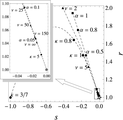
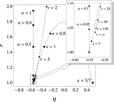
Figure 4: The current statefinder locations. The diagrams show the current positions for the Chaplygin gas model with CDM (circles), the GCG model (squares) and the SCG model (triangles). The star denotes the $\Lambda$CDM location. The areas bordered by the rectangles are enlarged to resolve the values near the $\Lambda$CDM location (star).

Nevertheless these trajectories are not of determining significance in themselves. The current statefinder values are of primary importance to differentiate cosmological scenarios from $\Lambda$CDM and to impose restrictions on the models. The figure 4 shows the current statefinder locations for the models with the Chaplygin gas assuming that the current DE density $\Omega_{\Lambda 0}=0.7$.

It is the sole parameter $\kappa$ determining the statefinder evolution trajectory and fixing the modern statefinder values in the model with the pure Chaplygin gas. We start with the value of $\kappa=3/7$ which coincides with the current ratio between DM and DE energy densities that leads to the modern statefinder values located far from the $\Lambda$CDM point. It is easy to see that already for $\kappa=5$ the modern location is fairly close to $\Lambda$CDM. In the GCG model one uses the decomposition of the energy density into two components

$$\rho=\rho_{\Lambda}+\rho_{\text{m}}\quad\text{and}\quad p=-\rho_{\Lambda}$$ (39)

proposed in [12] to fix the current statefinder position. The figure 4 shows that it approaches the $\Lambda$CDM point as $\alpha$ tends to zero.

The current values for the SCG model are given for fixed $k=0.2$ and different $\nu$. As one would expect, they are far from the $\Lambda$CDM point as well as from other models concerned when $\nu$ is small, and tend to the $\Lambda$CDM fixed point when $\nu$ increases.

The $s-r$ diagram demonstrates the very close trajectories for all three models near the $\Lambda$CDM point. In contrast, the $q-r$ diagram allows to differentiate between these models. In the GCG model the current deceleration factor is the same as in $\Lambda$CDM for any $\alpha$ owing to the selected decomposition (39). It implies that today’s statefinder locations for different $\alpha$ lies along the vertical line $q=\left(q_{0}\right)_{\Lambda\text{CDM}}=0.55$ in the $q-r$ diagram.

In the model with the pure Chaplygin gas

$$q_{0}=\left(q_{0}\right)_{\Lambda\text{CDM}}+\frac{3}{2}\,\frac{\kappa_{0}^{2}/\kappa^{2}}{1+\kappa_{0}}$$ (40)

and it is to be found resting on the parabola to the right of the vertical line.

When $\nu$ increases the current statefinder location line in the SCG model come close to the parabola since large $\nu$ means that the normal component behaves like CDM. Decreasing $k$ implies attenuation of interrelation between the components of SCG that also leads to the approach of the SCG and pure Chaplygin gas models and further degeneration SCG into $\Lambda$CDM.

Figure 5: The integrated statefinder locations. The diagrams show the integrated statefinder indices defined by (41) for the Chaplygin gas model with CDM (parabolas) for different $\kappa$ and the SCG model for different $\nu$ at $k=0.2$. The dashed lines corresponds to $z_{\text{max}}=1$, the dot-dashed lines corresponds to $z_{\text{max}}=2$, and the dotted lines contain the current locations. The values for $\kappa=1$ (circles) and 5 (squares), and $\nu=20$ (triangles) and 150 (rhombuses) are marked out for detail comparison. The stars denote the $\Lambda$CDM locations.

In order to distinguish these models with confidence we use the following integrated quantities

$$\bar{q}=\frac{1}{z_{\text{max}}}\int\limits_{0}^{z_{\text{max}}}\!\!q\,{\rm{d}}z\,,\quad\bar{r}=\frac{1}{z_{\text{max}}}\int\limits_{0}^{z_{\text{max}}}\!\!r\,{\rm{d}}z\,,\quad\bar{s}=\frac{1}{z_{\text{max}}}\int\limits_{0}^{z_{\text{max}}}\!\!s\,{\rm{d}}z\,,$$ (41)

introduced in [15] to take into account a previous DE evolution. The figure 5 depicts the lines passing through the points associated with the pairs $\{\bar{s},\bar{r}\}$ and $\{\bar{q},\bar{r}\}$ for different values of $\kappa$ in the pure Chaplygin gas model and for different $\nu$ in the SCG model. The current location lines are added for comparison. It is apparent that the certain values of $z_{\text{max}}$ considerably separates the models even though their current statefinder positions are almost indistinguishable. It is clear that in general an opposite situation can also take place. Because of this ambiguity the trend of $z_{\text{max}}$-dependence should be specially considered. The figure 6 shows the $\bar{s}-\bar{r}$ and $\bar{s}-\bar{r}$ diagrams governing by $z_{\text{max}}$. Magnitudes of the quantities (41) are less then the maximal corresponding statefinder values in the range $[0,z_{\text{max}}]$, and the evolution curves in the figure 3 are quite smooth, therefore the integrated statefinder trajectories are similar to the evolution ones and their efficiency could be developed in different ways. Since the SCG trajectories in the $\bar{q}-\bar{r}$ plane for large $\nu$ become closer to the $\Lambda$CDM line at greater $z_{\text{max}}$ then to increase $z_{\text{max}}$ is not so reasonable as to improve a statistical accuracy through a larger number of SNIa in the observational redshift range. To the contrary, the difference between the SCG model and $\Lambda$CDM in the $\bar{s}-\bar{r}$ diagram is enhanced when $z_{\text{max}}$ increases. It is primarily caused by a growing magnitude of the parameter $s$ in the SCG model up to the instant when $p_{\text{tot}}=0$ while $\Lambda$CDM is represented as the fixed point $\{0,1\}$ as in the current statefinder diagram. This advantage is favorable to distinguish the competing models with more confidence using observations of SNIa at higher redshifts. Similar estimations were carried out in [15], where the authors revealed that the discriminatory ability of the statefinders varies with redshift and showed that it improves when $q$, $r$ and $s$ in (41) are integrated over different redshift ranges.

Figure 6: $z_{\text{max}}$-dependence of the integrated statefinder quantities. The dot-dashed lines correspond to the Chaplygin gas model with CDM for $\kappa=5$. The dashed lines correspond to SCG model for $\nu=20$ (long dashes) and 150 (short dashes), and the dotted lines represent the statefinder evolution trajectories for the same parameters. $\Lambda$CDM is shown as the star in the left panel and the horizontal solid line in the right one. The values for $z_{\text{max}}=1$ (circles), 2 (squares) and 5 (rhombuses) are marked out for detail comparison.

5 Conclusion

In this letter the SCG model is studied from the statefinder viewpoint. This model describes the dark sector of the universe as a matter that behaves as DE while it is in the ground state and as DM when it is in the excited state. Cosmological dynamics is described in the framework of the relativistic superfluid model therefore the interaction between DE and DM is implicitly involved into the conservation laws (19) and (20).

The condensate possesses the equation of state of the Chaplygin gas but the universe evolution provided by this matter is different from the two-component model with the Chaplygin gas and CDM as well as from the GCG model used for unifying DE and DM. The discrimination is obviously demonstrated in the statefinder evolution diagrams. The diagrams show that for fixed ratio between DM and DE energy densities two quantities determine the trajectory and the current statefinder location. The former, $\nu$, governing the DM equation of state ought to be quite large to correspond to the cosmological observations. It implies that the pressure of the normal component is small and it behaves like CDM. From the superfluid standpoint it means that the second sound speed is small too and this inference should be taken into account for any (realistic or simulative) DM equation of state. The latter, $k$, interrelating the DM and DE is restricted for the universe commenced to accelerate before now. The limiting case of infinite $\nu$ and $k=0$ corresponds to $\Lambda$CDM and establishes the maximal value for the transition redshift $z_{\text{T}}=(z_{\text{T}})_{\Lambda\text{CDM}}=0.671$ in the SCG model.

Near the $\Lambda$CDM fixed point the SCG and pure Chaplygin gas models are close together but they can be separated if the earlier evolution is taken into account. It is found that the better evaluation could be developed at lower redshifts for the parameters $\bar{q}$ and $\bar{r}$, and at higher redshifts for $\bar{s}$. The same inference was made in [15] on the statefinder analysis of a number of models. As it is shown in [15] the observational data from the SNAP type experiments are in reasonably good agreement with $\Lambda$CDM and rule out the models whose current statefinder values locate far from the $\Lambda$CDM point. This is the reason that an effect of the previous DE evolution takes on great importance. It is hoped that the future high-z supernova observations will provide new data to clarify the essence of DE.

References

-
[1]
A. G. Riess et al., Observational Evidence from
Supernovae for an Accelerating Universe and a Cosmological
Constant, Astron. J. 116 (1998) 1009 [astro-ph/9805201];
S. Perlmutter et al., Measurements of and from 42 High-Redshift Supernovae, Astrophys. J. 517 (1999) 565 [astro-ph/9812133];
J. L. Tonry et al., Cosmological Results from High-z Supernovae, Astrophys. J. 594 (2003) 1 [astro-ph/0305008];
R. A. Knop et al., New Constraints on , , and from an Independent Set of Eleven High-Redshift Supernovae Observed with HST, Astrophys. J. 598 (2003) 102 [astro-ph/0309368].
-
[2]
S. Masi et al., The BOOMERanG experiment and the curvature
of the
Universe, Prog. Part. Nucl. Phys. 48 (2002) 243 [astro-ph/0201137];
C. L. Bennett et al., First Year Wilkinson Microwave Anisotropy Probe (WMAP) Observations: Preliminary Maps and Basic Results, Astrophys. J. Suppl. 148 (2003) 1 [astro-ph/0302207];
D. N. Spergel et al., First Year Wilkinson Microwave Anisotropy Probe (WMAP) Observations: Determination of Cosmological Parameters, Astrophys. J. Suppl. 148 (2003) 175 [astro-ph/0302209];
C. J. MacTavish et al., Cosmological Parameters from the 2003 flight of BOOMERANG, Astrophys. J. 647 (2006) 799 [astro-ph/0507503];
E. Komatsu et al., Seven-Year Wilkinson Microwave Anisotropy Probe (WMAP) Observations: Cosmological Interpretation, Astrophys. J. Suppl. 192 (2011) 18 [arXiv:1001.4538]. -
[3]
M. Tegmark et al., Cosmological parameters from SDSS and
WMAP, Phys. Rev. D 69 (2004) 103501 [astro-ph/0310723];
A. C. Pope et al., Cosmological Parameters from Eigenmode Analysis of Sloan Digital Sky Survey Galaxy Redshifts, Astrophys. J. 607 (2004) 655 [astro-ph/040124];
U. Seljak et al., Cosmological parameter analysis including SDSS Ly- forest and galaxy bias: constraints on the primordial spectrum of fluctuations, neutrino mass, and dark energy, Phys. Rev. D 71 (2005) 103515 [astro-ph/0407372];
K. Abazajian et al., The Seventh Data Release of the Sloan Digital Sky Survey, Astrophys. J. Suppl. 182 (2009) 543 [arXiv:0812.0649]. -
[4]
C. Wetterich, Cosmology and the fate of dilatation
symmetry, Nucl. Phys. B 302 (1988) 668;
P. J. E. Peebles and B. Ratra, Cosmology with a Time Variable Cosmological Constant, Astrophys. J. 325 (1988) L17. - [5] C. Armendariz-Picon, V. F. Mukhanov and P. J. Steinhardt, Dynamical Solution to the Problem of a Small Cosmological Constant and Late-Time Cosmic Acceleration, Phys. Rev. Lett. 85 (2000) 4438 [astro-ph/0004134].
- [6] R. R. Caldwell, M. Kamionkowski and N. N. Weinberg, Phantom Energy and Cosmic Doomsday, Phys. Rev. Lett. 91 (2003) 071301 [astro-ph/0302506].
-
[7]
C. Csaki, M. Graesser, L. Randall and
J. Terning, Cosmology of Brane Models with Radion
Stabilization, Phys. Rev. D 62 (2000) 045015 [hep-ph/9911406];
C. Deffayet, S. J. Landau, J. Raux, M. Zaldarriaga and P. Astier, Supernovae, CMB, and Gravitational Leakage into Extra Dimensions, Phys. Rev. D 66 (2002) 024019 [astro-ph/0201164]. - [8] A. Y. Kamenshchik, U. Moschella and V. Pasquier, An alternative to quintessence, Phys. Lett. B 511 (2001) 265 [gr-qc/0103004].
-
[9]
E. J. Copeland, M. Sami and S. Tsujikawa, Dynamics of
dark energy, Int. J. Mod. Phys. D 15 (2006) 1753 [hep-th/0603057];
J. Frieman, M. Turner and D. Huterer, Dark Energy and the Accelerating Universe, Ann. Rev. Astron. Astrophys. 46 (2008) 385 [arXiv:0803.0982]. -
[10]
A. R. Liddle and L. A. Urena-Lopez, Inflation, dark
matter and dark energy in the string
landscape, Phys. Rev. Lett. 97 (2006) 161301 [astro-ph/0605205];
S. Capozziello, S. Nojiri and S. D. Odintsov, Unified phantom cosmology: inflation, dark energy and dark matter under the same standard, Phys. Lett. B 632 (2006) 597 [hep-th/0507182];
N. Bose and A. S. Majumdar, A k-essence Model Of Inflation, Dark Matter and Dark Energy, Phys. Rev. D 79 (2009) 103517 [arXiv:0812.4131];
A. B. Henriques, R. Potting and P. M. Sa, Unification of inflation, dark energy, and dark matter within the Salam-Sezgin cosmological model, Phys. Rev. D 79 (2009) 103522 [arXiv:0903.2014];
J. De-Santiago and J. L. Cervantes-Cota, Generalizing a Unified Model of Dark Matter, Dark Energy, and Inflation with Non Canonical Kinetic Term, Phys. Rev. D 83 (2011) 063502 [arXiv:1102.1777]. -
[11]
M. C. Bento, O. Bertolami and A. A. Sen, Generalized
Chaplygin Gas, Accelerated Expansion and Dark Energy-Matter
Unification, Phys. Rev. D 66 (2002) 043507 [gr-qc/0202064];
N. Bilić, G. B. Tupper and R. D. Viollier, Unification of dark matter and dark energy: the inhomogeneous Chaplygin gas, Phys. Lett. B 535 (2002) 17 [astro-ph/0111325]. - [12] M. C. Bento, O. Bertolami and A. A. Sen, The revival of the unified dark energy-dark matter model?, Phys. Rev. D 70 (2004) 083519 [astro-ph/0407239].
- [13] V. A. Popov, Dark Energy and Dark Matter unification via superfluid Chaplygin gas, Phys. Lett. B 686 (2010) 211 [arXiv:0912.1609].
- [14] V. Sahni, T. D. Saini, A. A. Starobinsky and U. Alam, Statefinder – a new geometrical diagnostic of dark energy, JETP Lett. 77 (2003) 201 [astro-ph/0201498].
- [15] U. Alam, V. Sahni, T. D. Saini and A. A. Starobinsky, Exploring the Expanding Universe and Dark Energy using the Statefinder Diagnostic, Mon. Not. Roy. Ast. Soc. 344 (2003) 1057 [astro-ph/0303009].
- [16] B. R. Chang, H. Y. Liu, L. X. Xu, C. W. Zhang and Y. L. Ping, Statefinder parameters for interacting phantom energy with dark matter, JCAP 0701 (2007) 016 [astro-ph/0612616].
- [17] V. Gorini, A. Kamenshchik and U. Moschella, Can the Chaplygin gas be a plausible model for dark energy?, Phys. Rev. D 67 (2003) 063509 [astro-ph/0209395].
-
[18]
X. Zhang, Statefinder diagnostic for holographic dark
energy model, Int. J. Mod. Phys. D 14 (2005) 063509 [astro-ph/0504586];
M. R. Setare and M. Jamil, Statefinder diagnostic and stability of modified gravity consistent with holographic and new agegraphic dark energy, Gen. Rel. Gravit. 43 (2011) 293 [arXiv:1008.4763]. -
[19]
L. P. Chimento, A. S. Jakubi, D. Pavon and
W. Zimdahl, Interacting quintessence solution to the coincidence
problem, Phys. Rev. D 67 (2003) 083513 [astro-ph/0303145];
L. Zhang, J. Cui, J. Zhang, and X. Zhang, Interacting model of new agegraphic dark energy: Cosmological evolution and statefinder diagnostic, Int. J. Mod. Phys. D 19 (2010) 21 [arXiv:0911.2838];
A. Khodam-Mohammadi and M. Malekjani, Cosmic Behavior, Statefinder Diagnostic and Analysis for Interacting NADE model in Non-flat Universe, Astrophys. Space Sci. 331 (2011) 265 [arXiv:1003.0543]. -
[20]
Z. L. Yi and T. J. Zhang, Statefinder diagnostic for the
modified polytropic Cardassian universe, Phys. Rev. D 75 (2007) 083515 [astro-ph/0703630];
M. Tong, Y. Zhang and T. Xia, Statefinder parameters for quantum effective Yang-Mills condensate dark energy model, Int. J. Mod. Phys. D 18 (2009) 797 [arXiv:0809.2123];
H. Farajollahi and A. Salehi, Attractors, Statefinders and Observational Measurement for Chameleonic Brans–Dicke Cosmology, JCAP 1011 (2010) 006 [arXiv:1010.3589];
P. Wu and H. Yu, Observational constraints on theory, Phys. Lett. B 693 (2010) 415 [arXiv:1006.0674]. -
[21]
I. M. Khalatnikov and V. V. Lebedev, Relativistic
hydrodynamics of a superfluid
liquid, Phys. Lett. A 91 (1982) 70;
Sov. Phys. JETP 56 (1982) 923;
B. Carter, The Canonical Treatment of Heat Condition and Superfluidity in Relativistic Hydrodynamics, in A Random Walk in Relativity and Cosmology, Proceedings, Vadya Raychaudhuri Festschrift, I.A.G.R.G., 1983, Wiley Easter, Bombay (1985), pg. 48;
B. Carter and I. M. Khalatnikov, Momentum, vorticity, and helicity in covariant superfluid dynamics, Ann. Phys. (N.Y.) 219 (1992) 243;
B. Carter and I. M. Khalatnikov, Equivalence of convective and potential variational derivations of covariant superfluid dynamic, Phys. Rev. D 45 (1992) 4536. - [22] B. Carter and D. Langlois, The equation of state for cool relativistic two-constituent superfluid dynamics, Phys. Rev. D 51 (1995) 5855 [hep-th/9507058].
- [23] V. A. Popov, Relativistic Kinetics of Phonon Gas in Superfluids, Gen. Rel. Grav. 38 (2006) 917 [gr-qc/0607023].
-
[24]
A. G. Riess et al., Type Ia Supernova Discoveries at
From the Hubble Space Telescope: Evidence for Past
Deceleration and Constraints on Dark Energy
Evolution, Astrophys. J. 607 (2004) 665 [astro-ph/0402512];
F. Y. Wang and Z. G. Dai, Constraining Dark Energy and Cosmological Transition Redshift with Type Ia Supernovae, Chin. J. Astron. Astrophys. 6 (2006) 561 [arXiv:0708.4062];
W. M. Wood-Vasey et al., Observational Constraints on the Nature of the Dark Energy: First Cosmological Results from the ESSENCE Supernova Survey, Astrophys. J. 666 (2007) 694 [astro-ph/0701041];
E. E. O. Ishida, R. R. R. Reis, A. V. Toribio and I. Waga, When did cosmic acceleration start? How fast was the transition?, Astropart. Phys. 28 (2008) 547 [arXiv:0706.0546];
J. Lu, L. Xu, M. Liu and Y. Gui, Constraints on accelerating universe using ESSENCE and Gold supernovae data combined with other cosmological probes, Eur. Phys. J. C 58 (2008) 311 [arXiv:0812.3209].