Chapter 0 A Methodology for Optimizing Multithreaded System Scalability on Multi-cores

Neil Gunther1, Shanti Subramanyam2 and Stefan Parvu3 1Performance Dynamics Company, Castro Valley, California, USA
2Yahoo! Inc., Sunnyvale, California, USA
3Nokia, Espoo, Finland

Programming Multi-core and Many-core Computing SystemsS. Pllana and F. Xhafa (eds.)

1 Introduction

The ability to write efficient multithreaded programs is vital for system scalability, whether it be for parallel scientific codes or large-scale web applications. Scalability is about guaranteeing sustainable size, so it should be incorporated into initial system design rather than retrofitted as an afterthought. That requires a complete methodology which combines controlled measurements of the multithreaded platform together with a scalability modeling framework within which to evaluate those performance measurements.

In this chapter we show how scalability can be quantified using the Universal Scalability Law [gcap, usl] by applying it to controlled performance measurements of memcached, J2EE and Weblogic. Commercial multi-core processors are essentially black-boxes and although some manufacturers do offer specialized registers to measure individual core utilization [purr, corestat], not just overall processor utilization, the most accessible performance gains are primarily available at the application level. We also demonstrate how our methodology can identify the most significant performance tuning opportunities to optimize application scalability, as well as providing an easy means for exploring other aspects of the multi-core system design space.

The typical performance focus is on tools and techniques to profile and compile fine-grained parallel codes for scientific applications executing on many-core and multi-core processors. Here, however. we shall be concerned with performance at the other end of that spectrum, viz., system performance of concurrent, multithreaded applications as employed by commercial enterprises and large-scale web sites. Economies of scale dictate that these systems eventually be migrated to many-core and multi-core platforms.

Why is the emphasis on system performance important? Whatever the performance gains attained at the individual processor level, the impact of those gains must also be evident at the integrated system level so as to justify the cost of the effort. A fortiori, optimizing a local processor subsystem does not guarantee that the total system will also be optimized.

The claimed benefits of the various tools used for programming multi-core applications [ieee10, masspar, acm11] need to be evaluated quantitatively, not merely accepted as qualitative prescriptions [hetero, patterson]. It often happens that applications which are heralded as being multithreaded and scalable, turn out not to be when measured correctly [velocity]. To avoid setting incorrect expectations, system performance analysis should be incorporated into a comprehensive methodology rather than being done as an afterthought. We provide such a methodology in this chapter.

The organization of this chapter is as follows. In Sect. 2 we establish some of the terminology used throughout and the basic procedural steps for assessing system scalability. In Sect. 3 we review what it means to perform the appropriate controlled measurements. The design and implementation of appropriate load-test workloads for such controlled measurements is discussed in Sect. 4. Sect. 5 presents the universal scalability model that we use to perform statistical regression on the performance data obtained controlled measurements. In this way we are able to quantify scalability. In Sect. 6 we present the first detailed application of our methodology to quantify memcached scalability. In Sect. 7 we give some idea of how to extend our methodology to a multithreaded java application. Sect. 9 discusses some ideas about quantifying GPU and many-core scalability. The importance of our methodology for the often overlooked validation of complex performance measurements is presented in Sect. 8. Finally, Sect. 11 provides a summary and possible extensions to our methodology.

Although we shall focus on the broader issues of general-purpose, highly- concurrent, multithreaded and multi-core [ieee10] applications [shanti04], we anticipate that readers who are more involved with scientific applications will also be able to apply our methodology to their systems.

2 Multithreading And Scalability

We begin by presenting the context and terminology for comparing multi-threaded applications that either scale-out or scale-up.

Much of the FOSS stack used for running web applications e.g., memcached, MySQL, Ruby-on-Rails, has scalability limitations that are masked by the widespread adoption of horizontal scale-out. As traffic growth forces the necessity for more and cheaper multi-core servers, multithreading scalability becomes a significant issue once again.

Most web deployments have now standardized on horizontal scale-out in every tier—web, application, caching and database—using cheap, off-the-shelf, white boxes. In this approach, there are no real expectations for vertical scalability of server applications like memcached or the full LAMP stack. But with the potential for highly concurrent scalability offered by newer multi-core processors, it is no longer cost-effective to ignore the potential under utilization of processor resources due to poor thread-level scalability of the web stack.

Our USL methodology quantifies scalability using the following iterative procedure:

1. Measure the system throughput (e.g., requests per second) for a configuration where either the number of user-threads is varied on a fixed multi-core platform or the number of physical cores is varied using a fixed number of user-threads per core.

2. Measurements should include at least half a dozen data points in order to make the regression analysis statistically meaningful.

3. Calculate the capacity ratio $C(N)$ and efficiency $E(N)$ defined in Section 5.

4. Perform nonlinear statistical regression [regressR] to determine the USL scalability parameters $\alpha$, $\beta$ defined in Sect. 5.

5. Use the values of $\alpha$ and $\beta$ to predict $N_{c}$, where the scalability maximum is expected to occur. $N_{c}$ may lie outside any physically attainable system configuration.

6. The magnitude of the $\alpha$ parameter is associated with system contention effects (in the application, the hardware or both), and the $\beta$ parameter is associated with data coherency effects. This step provides the vital connection between the numerical output of the USL model and the identification of likely candidates for further performance tuning in software and hardware. See Sects. 6 and 8.

7. Repeat these steps with a new set of measurements until any differences between data and the USL projections are optimized.

We elaborate on each of these steps in the subsequent sections.

3 Controlled Performance Measurements

When doing scalability analysis of multithreaded applications, it is important to collect the data using controlled measurements. Controlled measurements require:

1. a controlled hardware platform that faithfully represents the real system being analyzed. The load-test platform that we used to perform the measurements presented in Sect. 6 is shown schematically in Fig. 1.

2. a well-designed workload together with tools that produce accurate data resulting in measurements that are repeatable. The workloads that we used are described in Sect. 4.

Figure 1: Schematic of scalability load measurement configuration.

The throughput results from a typical performance test are shown in Figure 2. A performance test is characterized by a “ramp-up” period in which load is increased on the system, a “steady-state” period during which performance data is gathered and a “ramp-down” period as the load diminishes.

It is important to ensure that the ramp-up period is sufficiently large to get the server performing operations in a normal manner, e.g., all data that is likely to be cached has been read in. This can require times ranging from a couple of minutes to several tens of minutes, depending on the complexity of the workload.

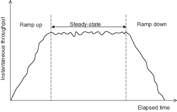
Figure 2: Steady state measurement of instantaneous throughput, for a particular load value $N$, represented as a time series to show the ramp up and ramp down phases.

The steady-state time should be sufficiently long to include all of the activity that may occur on the system during normal operations (e.g. garbage collection, writing to logs at some regular interval, etc.)

Scalability tests should ensure that the infrastructure is well-tuned and does not have inherent bottlenecks (e.g. incorrect network routes). This implies active monitoring of the test infrastructure and analysis of the data to ascertain it is accurate. Repeating the tests can also help to validate measurements.

4 Workload Design and Implementation

Data collected from controlled performance measurements are only as good as the workload used to run the tests. A poorly designed workload can result in irrelevant measurements and wrong conclusions [shanti04]. A well-designed workload should have the following characteristics:

Predictability:

The behavior of the system while running the workload, should be predictable. This means that one should be able to determine how the workload processes requests and accesses data. This helps in analyzing performance.

Repeatability:

If the workload is run several times in an identical fashion, it should produce results that are statistically identical. Without this repeatability, performance analysis becomes difficult.

Scalability:

A workload should be able to place different levels of load in order to test the scalability of the target application and infrastructure. A workload that can only generate a fixed load or one that scales in an haphazard fashion that does not resemble actual scaling in production is not very useful.

These characteristics can be realized using the following design principles:

Design the interactions:

Define the actors and their use cases. The use cases help define the operations of the workload. In a complex workload, the different actors may have different use cases, e.g., a salesperson entering an order and an accountant generating a report. Combine use cases that are likely to occur together into a workload. For example, batch operations run at night should be a separate workload from online, interactive operations.

Define the metrics:

Typical metrics include throughput (number of operations executed per unit time) and response time. Response time metrics are usually specified as average, 90th or 95th percentiles.

Design the load:

This means defining the manner by which the different operations associated with the metrics offer load onto the servers. This involves deciding on the operation mix, mechanisms to generate data for the requests, and deciding on arrival rates or think times. This step is crucial to get right if the workload needs to emulate a production system and/or is being used for performance testing of the important code paths in the application. A slow operation that is executed only 1% of the time can sometimes be ignored whereas even a 5% drop in performance of an operation that occurs 50% of the time may be not be tolerable.

Define scaling rules:

This step is often overlooked, leading to overly optimistic results during testing. Complex workloads need a means by which to scale the workload depending on the actual deployment hardware. Often, scaling is done by increasing the number of emulated users/threads. Any data-dependent application also needs to have the data-set scaled in order to truly measure the performance impact of a large number of concurrent users.

With regard to workload implementation, there exist several open-source and commercial tools that aid in the development of workloads, and running them. Available tools vary considerably in functionality, ability to scale, and their own performance overhead. Some preliminary investigations may be necessary to ensure that a given choice of tool can meet the anticipated requirements.

5 Quantifying Scalability

There are many well known techniques for achieving better scalability: collocation, caching, pooling, and parallelism, to name a few. But these are only qualitative descriptions. How can one decide on the relative merits of any of these techniques unless they can be quantified? This is clearly a role for performance modeling. Performance models are essential, not only for prediction but, as we discuss in Sects. 6 and 8, for interpreting scalability measurements.

Many performance modeling tools, such as event-based simulators and analytic solvers, are based on a queueing paradigm that requires measured service times as modeling inputs. More often than not, however, such measurements are unavailable, thereby thwarting the use of these modeling tools. This is especially true for multi-tier, web-based applications. A more practical intermediate approach is to apply nonlinear regression [regressR] to performance measurements that are more accessible; the major advantage being that service-time measurements are not required.

1 Queueing Model Foundations

The universal scalability model (or USL model) that we present in this section is a realization of the approach alluded to in the previous section. The USL is a nonlinear parametric model [gcap, usl] derived from a well defined queue-theoretic model known as the machine repairman model [gross, ppdq].

Elementary $M/M/m$ queueing models [ppdq] of multi-cores and multithreaded systems are too simple because they allow an unbounded number of requests to occupy the system and they cannot account for processor-to-processor interactions. Machine-repairman models, like $M/G/m/N/N$, are defined to have only a finite number of requests [ppdq]. That constraint can be used to reflect the finite number of threads in a load test platform, as discussed on Sects. 3 and 4. Alternatively, $M/G/m/N/N$ models can represent the interactions between $N$ processors [balbo]. Indeed, the machine repairman model can be further generalized in terms of queueing network models to analyze the performance of parallel systems [sevcik], including architectures with multiple latency stages [pdcs05], provided the requisite service times can be measured.

Table 1: Interpretation of $M/M/1/N/N$ queueing metrics

Metric	Repairman	Multi-core	Multi-thread
N	machines	virtual processors	user threads
Z	up time	execution period	think time
S	service time	transmission time	processing time
W	wait time	interconnect latency	scheduling time
X	failure rate	bus bandwidth	throughput

Here, we restrict ourselves to the $M/M/1/N/N$ queueing model where the single Markovian server represents the interconnect latency between $N$ processors or cores. Since the components of this queue have a consistent physical interpretation with respect to multi-core performance metrics (Table 1), we also avoid mere curve fitting exercises with ad hoc parameters.

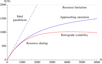
Figure 3: Physical components of scalability.

To motivate our choice of performance model, we briefly review the key physical attributes of scalability. Referring to Fig. 3:

1. Ideal parallelism: Linear scaling corresponds to equal bang for the buck computational capacity where each increment in the load, $\Delta N$ on the $x$-axis, produces a constant increment in throughput, $\Delta X$ on the $y$-axis, as indicated by the dashed inclined line in Fig. 3. Such linearity in capacity can be written symbolically as:

   $$C(N)=N$$ (1)

   This includes scaled sizing of the workload [gcap].

2. Resource sharing: Accounts for the fall away from linear scaling due to waiting for access to shared resources. This loss of linearity due to resource contention is associated with the USL model parameter

   $$0<\alpha<1$$ (2)

3. Resource limitation: Even if such linear scaling is achievable, it cannot exceed the finite capacity of the system resources. This is defined by an asymptotic bound from above:

   $$\lim_{N\rightarrow\infty}C(N,\alpha)=\frac{1}{\alpha}$$ (3)

   This saturation limit is shown as the dashed horizontal line in Fig. 3. This bound could be lower due to execution-time skew in components of the workload [ppa, cilk].

4. Retrograde scaling: Worse than saturation, this effect arises from the additional latency due to pairwise interprocessor communication, e.g., exchange of data between caches, and is given by the binomial coefficient:

   $$\binom{N}{2}=\dfrac{N(N-1)}{2}$$ (4)

   and is associated with a USL parameter $\beta$.

Another useful metric is the efficiency:

$$E(N)=\dfrac{C(N)}{N}$$ (5)

which defines the scalability (11) per core or per thread. We shall apply this metric to data validation in Sect. 8.

2 Universal Scalability Model

The following theorem allows us to combine each of the physical scalability components of Sect. 1 into a parametric model.

Definition 1 (Universal Scalability Law)

$$C(N,\alpha,\beta)=\dfrac{N}{1+\alpha(N-1)+\beta N(N-1)}$$ (6)

where the factor of 2 in (4) has been absorbed into the $\beta$ coefficient.

Theorem 1 (Queueing Bound)

The USL model (6) is equivalent to the synchronous bound on the throughput of a machine-repairman queueing model with a service time that is linearly load-dependent on $N$.

The formal proof is too long to reproduce here. A pivotal observation [gcap] is that for $M/M/1/N/N$, the throughput $X(N)$ is bounded below by:

$$X(N)\geq\dfrac{N}{NS+Z}$$ (7)

in the notation of Table 1. It also excludes super-linear scaling [sevcik, cilk].

Proof 1 (Sketch)

When the first request is in service (at the repairman) the mean waiting time for the remaining requests is

$$W=(N-1)S$$ (8)

where $N$ is the number of requests in the system. Let the service time be linearly load-dependent:

$$S(N)=cNS$$

with $c$ a constant of proportionality. For synchronous queueing all requests are enqueued simultaneously, so we can rewrite (8) as:

$$W=cN(N-1)\,S$$ (9)

Expressed as relative relative throughput, (9) appears in the denominator of (6) as the corresponding quadratic term.

The interested reader is referred to Ref. [usl] for the details and Ref. [zones] for supporting simulation results.

Perhaps the most important point for our methodology is that (6) is a mean value equation in the queueing variables and, in that sense, accounts for the possibility of fluctuations in the size of workload components and sub-tasks. In particular, the machine repairman model has been proven to be robust to fluctuations in these queue variables [gross].

Corollary 1 (Duality)

The scaling variable $N$ in the parametric model (6) can be interpreted equally as representing a finite number of threads (software view) or a finite number of core processors (hardware view) because it is a bound on same the $M/M/1/N/N$ queueing model.

Setting $\beta=0$ in (6) produces the standard parametric version of Amdahl’s law with (2) the serial fraction of the workload. However, by virtue of Theorem 1, Amdahl’s law can be interpreted as a limiting case (zero coherency delays) of the USL.

Corollary 2 (Amdahl’s Law)

Amdahl’s law corresponds to the relative throughput (speedup) due to synchronous queueing in the standard machine repairman queueing model with constant mean service time.

Amdahl’s law is the synchronous throughput bound on an $M/M/1//N$ queue having a load-independent mean service time S.

Proof 2 (Sketch)

The proof relies on the identity:

$$\alpha=\dfrac{S}{S+Z}\rightarrow\begin{cases}0&\text{as}~{}S\rightarrow 0,~{}\text{with}~{}Z=\text{const.},\\ 1&\text{as}~{}Z\rightarrow 0,~{}\text{with}~{}S=\text{const.}.\end{cases}$$ (10)

between the queueing metrics in Table 1 and the parameter $\alpha$ in (2).

See Appendix A of Ref. [gcap] and Ref. [usl] for a more detailed discussion.

An important point to note from the preceding is that Amdahl’s law represents worst case queueing effects [ieee08, isca]. This is consistent with the notion that synchronous requests have longer delays than asynchronous requests. The latter being the mean value throughput for $M/M/1//N$. Other examples of applying (6) to both hardware and software scalability, can be found in [gcap].

The capacity ratio for measured data is defined as the normalization:

$$C(N)=\frac{X(N)}{X(1)}$$ (11)

Since the capacity ratio has two definitions—one empirical (11) and the other analytical (6)—the optimization goal is to match them in such a way that the adjusted USL coefficients provide the best fit the performance data.

The key distinction is that, unlike Amdahl’s law, (6) possesses a maximum at

$$N_{c}=\sqrt{\frac{1-\alpha}{\beta}}$$ (12)

the location of which is controlled by the USL coefficients according to:

1. $N_{c}\rightarrow 0$ as $\alpha\rightarrow 1$

2. $N_{c}\rightarrow 0$ as $\beta\rightarrow\infty$

3. $N_{c}\rightarrow\infty$ as $\beta\rightarrow 0$

4. $N_{c}\rightarrow\beta^{-1/2}$ as $\alpha\rightarrow 0$

The important implication for our methodology is that beyond $N_{c}$ the throughput becomes retrograde. See Fig. 3. This effect is commonly observed in applications that involve shared-writable data.

Summarizing the steps for application optimization:

1. Steady state measurements of throughput $X(N)$ for each load point $N$.

2. At least half a dozen $N$ values are required in order to be statistically significant for USL fitting.

3. Calculate the capacity ratio (11) for each $N$ value.

4. Use nonlinear statistical regression [regressR] to determine the USL coefficients $\alpha$ and $\beta$.

5. Optimize the complete scalability function (6) for any desired $N$ value.

The same methodological procedure can be applied to hardware scalability optimization although, as we pointed out in the introduction, most commodity hardware is now a silicon black-box which mean the hardware performance tuning opportunities are far fewer.

The use of the term “universal” in this context refers not only to the general applicability of (6) to both multi-core hardware and multi-threaded software scalability, but also to the fact that no more than two coefficients are needed to accommodate the possibility of reaching saturation limits (Amdahl scaling) or thrashing limits (coherency delays). in the latter case, there is little virtue on modeling such degraded performance; better to try and improve it.

We now present some case studies that demonstrate how this methodology has been successfully applied.

6 Case Study: Memcached Scalability

As mentioned in Sect. 2, most large-scale web sites have standardized on horizontal scale-out in every tier as a simple way to achieve high degrees of scalability. A ubiquitous application used in this context is memcached (MCD). In this section, we demonstrate how are our analysis leads to improved thread scalability of MCD [velocity].

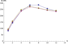
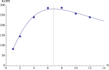
Figure 4: Throughput of three MCD releases up $N=12$ threads.

Figure 5: USL regression analysis of memcached 1.2.8 data (dots) in Fig. 5.

Figure 5 shows controlled MCD throughput as a function of $N\leq 12$ threads for three release: 1.2.8, 1.4.1 and 1.4.5, measured in thousands of operations/sec (KOPS). Each release has a very similar retrograde throughput profile, peaking between $N=6$ and $N=7$ threads.

Whereas the lines in Fig. 5 merely associate data points belonging to the same MCD release, the curve in Fig. 5 is generated by statistically fitting (6) to those data and is not required to pass through every data point.

The USL regression analysis of MCD 1.2.8 reveals a contention parameter value of $\alpha=0.0255$ and a coherency parameter value of $\beta=0.0210$. Repeating this procedure with the other MCD versions results in the USL coefficients summarized in Table 2. In this way, the scalability of MCD is now fully quantified. It is also clear that it would be desirable to move the estimated maximum at $N_{c}\approx 6$ to a higher value.

Table 2: Memcached scalability parameters

Version	$\alpha$	$\beta$	$N_{c}$
1.2.8	0.0255	0.0210	6.8121
1.4.1	0.0821	0.0207	6.6591
1.4.5	0.0988	0.0209	6.5666

Fig. 7 shows how scalability improved after various code changes were applied. This is where the procedural steps of our USL methodology, outlined in Sect. 2, actually pay off.

Access to the MCD cache is controlled by a single mutex lock. When running with greater than $6$ threads, contention for this mutex increases dramatically. A partitioned cache was implemented with each partition controlled by its own mutex. In addition, contention for the stats lock was identified. This lock controls access to the stats structure that is updated on every request. The stats structure was redesigned to hold stats on a per-thread basis. This fix was applied in release 1.4.5 and they greatly improved scalability.

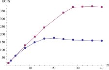
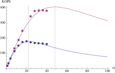
Figure 6: Comparison of scalability data for standard MCD (lower curve) and patched MCD (upper curve).

Figure 7: USL model of patched MCD data in Fig. 7 extended out to $N=100$ threads.

The USL fit to the patched MCD data in Fig. 7 is extended out to $N=100$ threads in Fig. 7. The original scalability peak at $N_{c}=22$ threads (lower curve) is now moved out to $N_{c}=48$ threads (upper curve).

At this point, the reader may be dumbstruck as to how the actual changes made to the application code are determined from the seemingly abstract numerical output of the USL model. First, it is important to recall that the role of the performance analyst is to measure and validate, not to modify hardware or software for which he or she was not responsible in the first place. That is the role of the hardware engineer or the software developer.

Second, the interpretation of the USL analysis and the choice of performance tuning optimization arises from discussions between the performance analyst and the appropriate engineers. Since the latter are the real experts, it is helpful if the modeling analysis can point to specific types of effects that may be contributing to inferior scalability. This is precisely what the USL does by virtue of its parameters having explicit physical meaning, viz., the respective degrees of concurrency ($N$), contention ($\alpha$), and coherency ($\beta$).

In this way, step 6 of the USL methodology in Sect. 2 can evoke a “light bulb” moment for engineers. In practice, we have seen this synergy occurring time and again. Moreover, the corrective action taken is usually something we, as performance analysts, could never have foreseen because we were not in possession of the implementation details. Although we have presented an example of improvements made to MCD software, Corollary 1 implies it could also have been that scalability improvements came from hardware changes, such as memory resizing or more recent revisions to the multicore architecture. That said, no matter what insights are favored or what tuning actions are adopted, the ultimate arbiter is the next iteration of the USL methodology.

7 Other Multi-threaded Applications

We focused on memcached scalability in Sect. 6 to demonstrate how the USL methodology is applied in detail. In this section, we show how the same methodology can be applied to other multi-threaded applications.

Java Enterprise Edition (J2EE) applications are extremely popular in enterprises because the J2EE platform is known to be robust, secure and scalable [shanti05].

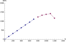
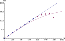
Figure 8: Initial J2EE throughput data (left) and subsequent data (right) measured in requests per second (RPS).

Figure 9: USL models of J2EE scalability for initial data (uppsr curve) and subsequent data (lower curve).

Figure 9 shows how the application throughput scales when load is added to a J2EE server. The blue and red points show different data sets to exhibit how the USL regression values change accordingly. See Table 3.

Table 3: J2EE application scalability parameters

Load	$\alpha$	$\beta$	$N_{c}$
Low	$1.49\times 10^{-5}$	$6.7\times 10^{-9}$	12216.90
High	0.0	$2.4\times 10^{-7}$	2041.24

When the USL is applied to the blue data points, it results in the upper curve in Fig. 9, which indicates excellent scalability up to more than $N_{c}\approx 12,000$ users. This modeling result is reasonable as the initial data set shows almost linear scalability through $N=800$ users.

However, consider what happens when the data set changes. As the load was increased and the red data points in Fig. 9 were measured, the corresponding USL parameters change accordingly resulting in the lower curve of Fig. 9. The larger $\beta$ value in Table 3 reflects a substantial decrease in predicted scalability. However, even that scalability is still extremely good (cf. the corresponding $\alpha$, and $\beta$ for MCD in Table 2), but instead of simply appealing to qualitative descriptions like “highly scalable,” or “great performance,” the USL coefficients provides us with true quantification of J2EE scalability.

We want to underscore that what looks like a bad prediction is, in fact, precisely how our methodology should work. Based on the initial data, maximum scalability was estimated to occur at $N_{c}\approx 12,000$ user threads. Further measurements, however, show that this maximum occurs at $N_{c}\approx 2,000$ user threads instead. It is not that the original USL projections were wrong, but that those initial data did not contain any information about a subsequent scaling limitation present in the JVM. The important point is that the USL sets expectations and then forces performance engineers to explain subsequent deviations at each stage of the measurement process.

8 Case Study: Data Validation

Another simple and immediate practical benefit of applying the methodology is validation of performance data.

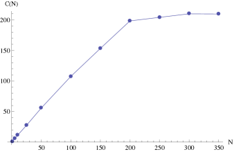
Figure 10: Web application scalability data.

Consider a test environment, similar to that described in Sects. 4 and 7, where test scripts are developed using different test cases for a particular application. In this case, the test configuration used Apache Jakarta JMeter as a load injector for a J2EE application [shanti05] running on Java 6 with a Weblogic application server. We are not interested in what this application was doing internally but rather, to examine and validate the load testing procedure.

Several tests were run against this J2EE application and the reported JMeter values were recorded. As usual, we were interested in the throughput and response time metrics. Following Sect. 2, throughout was the primary metric of interest for determining application scalability. Fig. 10 shows an example of the throughput data. It appears acceptable because:

• The data points are monotonically increasing. A sequence of numbers is monotonically increasing if each element in the sequence is larger than its predecessor. Notice that the profile appears to decrease slightly beyond $N=300$. The USL is designed to model such a characteristic.

• The sequence is linear-rising up to $N=200$ virtual users.

• The throughput reaches saturation around $N=300$. This is exactly what we expect for a closed queueing system [ppdq] with a finite number of active requests (as is true for any load-testing or benchmarking system). In this case, the onset of saturation looks rather sudden as indicated by the discontinuity in the gradient (“sharp knee”) at $N=200$. This is usually a sign of significant internal change in the dynamics of the combined hardware-software system.

These data seem to pass the visualization test and most performance testing would stop here. Unfortunately, visualization alone is not always sufficient proof of optimal scalability. Applying our USL methodology, we modeled these data to evaluate the $\alpha$ and $\beta$ coefficients and determine if application scalability could further be improved.

In setting up the USL model to perform statistical regression, we detected some efficiencies (5) that were greater than 100%. In particular, Table 4 exhibits $E(N)>1$ for test loads in the range $N=5$ to $150$ virtual users.

Table 4: Preparation for USL analysis of the data in Fig. 10

$N$	$C(N)$	$E(N)$
1	1.00	1.00
5	5.67	1.13
10	11.33	1.13
25	27.50	1.10
50	55.83	1.12
100	107.50	1.08
150	153.33	1.02
200	198.33	0.99
250	204.17	0.82
300	210.00	0.70
350	209.67	0.60

From a logical standpoint, we cannot have more than $100\%$ of anything. Sometimes, however, there are conventions in performance analysis where quantities exceeding $100\%$ have a particular interpretation, e.g., 3200% processor capacity might be shorthand for a maximal machine utilization of $32$ cores running at $100\%$ busy. Conventions notwithstanding, any numbers that are out of bounds should be flagged for explanation by performance engineers or application developers.

Axiom 1

Data + Models = Insight

All measurements contains errors and the more complex the measurement system, the more prone it will be to generating erroneous performance data. Without a validation framework, how can it be known when the data are wrong? The USL provides a simple mathematical reference framework for detecting anomalies like those in Table 4. We encapsulate this observation in Axiom 1 .

So, what was causing the excessive efficiencies in this case? Since we had not even invoked statistical regression at that point, we knew that the culprit could not be the USL model. Instead, it became clear that something was amiss with the measurement process. (Not the usual conclusion) The performance engineers then set about eliminating one factor at a time. Eventually, it emerged that the JMeter tool itself was the only remaining explanation for the source of the erroneous measurements. Without being forced by the USL modeling framework to resolve this unforeseen issue, further load testing would have been a waste of time and resources.

9 Scalability on Many-core Architectures

Tools for writing applications for CPU-GPU many-cores are constantly improving. Measuring and quantifying many-cores scalability of such applications is the next step and that requires a methodology, not just tools. In this section we indicate how the USL methodology can be applied to workloads running on many-core architectures.

1 Trends in Multiprocessing, Multi-cores and Many-cores

In recent years, vendors have been considering multi-core architectures and how applications can be migrated from single processors to multiple processors. In this paradigm, the multi-core forces the application programmer to focus on maintaining and maximizing execution speed of a sequential workload but replicating it across multiple processing units inside the same physical processor [masspar].

A different approach, using many-cores, focuses on how to maximize the aggregate throughput; an essential requirement for the gaming industry and anything else involving 3D graphics. This many-core approach deploys a much higher number of cores per physical processor unit, without the need for internal cache memories, logic control unit for executing instructions, and other complexities associated with multicore processors.

These alternative paradigms allow developers to consider which is the best option for their applications. Recent improvements offer additional mechanisms to select and direct parts of the application to either CPU or GPU, depending of its intended usage. Compute-intensive sections can be dynamically directed to a many-cores processor, while single-threaded sections can be assigned to a multicore processor. Such combinations of CPU and GPU, let the workloads run optimally by taking intelligent advantage of the type of processor hardware available.

However, not all applications are written to take advantage of these new architectures. For example, legacy single-threaded workloads typically cannot make use of these new options. When executed on many-core processors, such workloads will underperform.

Without significant modification and porting effort, legacy workloads cannot scale well. Testing and analyzing these workloads in a controlled fashion (see Sect. 3) is a necessity and presents another opportunity for our USL methodology.

2 USL Methodology for GPUs

Since the USL methodology is generic, it should be applicable to quantifying the scalability of many-core applications. In this vein, we have applied it to data kindly provided to us by Prof. Frank Dehne and Kumanan Yogaratnam at Carleton University [cangpu].

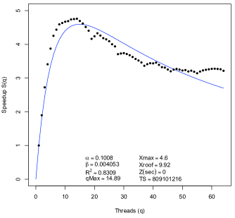
Figure 11: USL fit to nVIDIA Tesla GPU data.

They compare the speedup of different parallel graph algorithms running on an nVIDIA GeForce 260 with 216 2.1 GHz GPU-cores and 896 MB of RAM. The parallel speedup is logically equivalent to $C(N,\alpha,\beta)$ in the USL formalism.

Their choice of parallel graphing algorithms reveal irregular data access patterns (shown as dots in Fig. 11) that are different from than regular data access patterns found in typical parallel processing workloads for image processing, linear algebra or scientific computing. More importantly, significant speedup degradation is observed for $N>15$ threads.

10 Future Work

Applying USL regression analysis to the data in Sect. 9 produces the curve in Fig. 11, which has a contention parameter value of $\alpha=0.1008$ and a coherency parameter value of $\beta=0.00405$, with an estimated maximum at $N_{c}=14.89$ threads. The interpretation of these coefficients is still under investigation for potential ways to improve GPU scalability. In the meantime, the important point is that these controlled measurements are being compared with the USL performance model, thereby reinforcing Axiom 1.

Another avenue of research is using multi-cores to model multi-cores. The USL model is an excellent candidate for running thousands of simultaneous regressions in parallel and then selecting an optimal set of coefficients from the simulation results. Moreover, since the foundations of the USL lie in queue-theoretic models this approach could be extended to Monte Carlo simulations [mcR] of Markov models.

11 Concluding Remarks

In this chapter, we have presented a performance methodology for quantifying application scalability on multi-core and many-core systems. With potentially massive computational horsepower now being delivered in low-cost silicon black boxes, the remaining opportunities for improving performance lie mostly in the application layers.

Our methodology, based on the universal scalability law (USL), emphasizes the importance of validating scalability data through controlled measurements that use appropriately designed test workloads. These measurements must then be reconciled with the USL performance model. It is this synergy between measuring and modeling that provides the key to achieving successful scalability on multi-core platforms.

In Sect. 5 we presented the USL model and showed how it can be combined with nonlinear statistical regression to analyze controlled performance measurements. In this way, we are able to truly quantify scalability and thereby assess the cost-benefit of multithreaded applications running on multi-core or many-core architectures. The USL methodology also provides data validation as a side-effect of preparing for the more sophisticated regression analysis.

In Sect. 9 we presented some initial results from quantifying GPU and many-core scalability using the USL methodology. Possible confounding effects between the USL coefficients due to these fine-grained parallel workloads suggests an analysis based on the concept of scalability zones [zones].

With ever-increasing economies of scale offered by commodity multi-core to many-core systems, we anticipate that cost-benefit analysis tools, such as the USL-based methodology described here, to play an increasingly important role in the future of computing.

wileychap wileychap