Clustering, percolation and directionally convex ordering of point processes

Abstract

Heuristics indicate that point processes exhibiting clustering of points have larger critical radius $r_{c}$ for the percolation of their continuum percolation models than spatially homogeneous point processes. It has already been shown, and we reaffirm it in this paper, that the $dcx$ ordering of point processes is suitable to compare their clustering tendencies. Hence, it was tempting to conjecture that $r_{c}$ is increasing in $dcx$ order. Some numerical evidences support this conjecture for a special class of point processes, called perturbed lattices, which are “toy models” for determinantal and permanental point processes. However the conjecture is not true in full generality, since one can construct a Cox point process with degenerate critical radius $r_{c}=0$, that is $dcx$ larger than a given homogeneous Poisson point process, for which this radius is known to be strictly positive. Nevertheless, the aforementioned monotonicity in $dcx$ order can be proved, for a nonstandard critical radius ${\overline{r}}_{c}$ (larger than $r_{c}$), related to the Peierls argument. Moreover, we show the reverse monotonicity for another nonstandard critical radius ${\underline{r}}_{c}$ (smaller than $r_{c}$). This gives uniform lower and upper bounds on $r_{c}$ for all point processes $dcx$ smaller than some given point process. Moreover, we show that point processes $dcx$ smaller than a homogeneous Poisson point process admit uniformly non-degenerate lower and upper bounds on $r_{c}$. In fact, all the above results hold under weaker assumptions on the ordering of void probabilities or factorial moment measures only. Examples of point processes comparable to Poisson point processes in this weaker sense include determinantal and permanental point processes with trace-class integral kernels. More generally, we show that point processes $dcx$ smaller than a homogeneous Poisson point processes exhibit phase transitions in certain percolation models based on the level-sets of additive shot-noise fields of these point process. Examples of such models are $k$-percolation and SINR-percolation.

and

1 Introduction

Heuristic

Consider a point process $\Phi$ in the $d$-dimensional Euclidean space $\mathbb{R}^{d}$. For a given “radius” $r\geq 0$, let us join by an edge any two points of $\Phi$, which are at most at a distance of $2r$ from each other. Existence of an infinite component in the resulting graph is called percolation of the continuum model based on $\Phi$. Clustering of $\Phi$ roughly means that the points of $\Phi$ lie in clusters (groups) with the clusters being well spaced out. When trying to find the minimal $r$ for which the continuum model based on $\Phi$ percolates, we observe that points lying in the same cluster of $\Phi$ will be connected by edges for some smaller $r$ but points in different clusters need a relatively higher $r$ for having edges between them. Moreover, percolation cannot be achieved without edges between some points of different clusters. It seems to be evident that spreading points from clusters of $\Phi$ “more homogeneously” in the space would result in a decrease of the radius $r$ for which the percolation takes place. This is a heuristic explanation why clustering in a point process $\Phi$ should increase the critical radius $r_{c}=r_{c}(\Phi)$ for the percolation of the continuum percolation model on $\Phi$, called also the Gilbert’s disk graph or the Boolean model with fixed spherical grains.

Clustering and $dcx$ order

To make a formal conjecture out of the above heuristic, one needs to adopt a tool to compare clustering properties of different point processes. In this regard, we use directionally convex ($dcx$) order in this article. The $dcx$ order of random vectors is an integral order generated by twice differentiable functions with all their second order partial derivatives being non-negative. Its extension to point processes consists in comparison of vectors of number of points in every possible finite collection of bounded Borel subsets of the space. Our choice has its roots in [Błaszczyszyn and Yogeshwaran(2009)], where one shows various results as well as examples indicating that the $dcx$ order on point processes implies ordering of several well-known clustering characteristics in spatial statistics such as Ripley’s K-function and second moment densities. Namely, a point process that is larger in the $dcx$ order exhibits more clustering, while having the same mean number of points in any given set.

Conjecture

The above discussion tempts one to conjecture that $r_{c}$ is increasing with respect to the $dcx$ ordering of the underlying point processes; i.e., $\Phi_{1}\leq_{dcx}\Phi_{2}$ implies $r_{c}(\Phi_{1})\leq r_{c}(\Phi_{2})$. Since the critical radius $r_{c}$ for the percolation does not seem to have any explicit representation as a $dcx$ function of vectors of number of points in a finite collection of bounded Borel subsets, we are not able to compare straightforwardly $r_{c}$ of $dcx$ ordered point processes. At the same time, numerical evidences gathered for a certain class of point processes, called perturbed lattice point processes, were supportive of this conjecture. But as it turns out, the conjecture is not true in full generality and we will present a counter-example.

Counterexample

More specifically, for a given Poisson point process, we will construct a $dcx$ larger than it Poisson-Poisson cluster point process (a special case of doubly-stochastic Poisson, called also Cox, point process), whose critical radius is null (hence smaller than that of the given Poisson point process, which is known to be positive). In this Poisson-Poisson cluster point process points concentrate on some carefully chosen larger-scale structure, which itself has good percolation properties. In this case, the points concentrate in clusters, however we cannot say that clusters are well spaced out. Hence, this example does not contradict our initial heuristic explanation of why clustering in a point process should increase the critical radius for the percolation. It reveals rather, that $dcx$ ordering, while being able to compare the clustering tendency of point processes, is not capable of comparing macroscopic structures of clusters.

Comparison results

What we are able to do with $dcx$ order is to compare some nonstandard critical radii ${\overline{r}}_{c}$ and ${\underline{r}}_{c}$ related, respectively, to the finiteness of the expected number of void circuits around the origin and asymptotic of the expected number of long occupied paths from the origin in suitable discrete approximations of the continuum model. These new critical radii sandwich the “true” one, ${\underline{r}}_{c}(\Phi)\leq r_{c}(\Phi)\leq{\overline{r}}_{c}(\Phi)$. We show that if $\Phi_{1}\leq_{dcx}\Phi_{2}$, then as suggested by the heuristic, ${\overline{r}}_{c}(\Phi_{1})\leq{\overline{r}}_{c}(\Phi_{2})$. However, we obtain the reversed inequality for the other nonstandard critical radius: ${\underline{r}}_{c}(\Phi_{1})\geq{\underline{r}}_{c}(\Phi_{2})$. This reversed inequality can be also explained heuristically, by noting that whenever there is at least one path of some given length in a point process that clusters more, there might be actually so many such paths, that the inequality for the expected numbers of paths are reversed. However, as we have mentioned above, the fact is that there are examples of $dcx$ ordered point processes, for which the inequality is reversed for the critical radius $r_{c}$ itself, namely examples of $\Phi_{1}\leq_{dcx}\Phi_{2}$ with $r_{c}(\Phi_{1})>r_{c}(\Phi_{2})$.

Non-trivial phase transitions

A more positive interpretation of the aforementioned results is as follows. Combining the two opposite inequalities, we obtain as a corollary that if $\Phi_{1}\leq_{dcx}\Phi_{2}$ then the usual critical radius of the $dcx$ smaller point process can be sandwiched between the two nonstandard critical radii of the larger one,

$${\underline{r}}_{c}(\Phi_{2})\leq{\underline{r}}_{c}(\Phi_{1})\leq r_{c}(\Phi_{1})\leq{\overline{r}}_{c}(\Phi_{1})\leq{\overline{r}}_{c}(\Phi_{2}).$$

In more loose terms, the above result can be rephrased as follows: if a point process $\Phi_{2}$ exhibits the following double phase transition $0<{\underline{r}}_{c}(\Phi_{2})\leq{\overline{r}}_{c}(\Phi_{2})<\infty$, stronger than the usual one ($0<r_{c}(\Phi_{2})<\infty$), then its two nonstandard critical radii act as non-degenerate bounds on the critical radius $r_{c}(\Phi)$, uniformly valid over all $\Phi\leq_{dcx}\Phi_{2}$, thus in particular implying the usual phase transition $0<r_{c}(\Phi)<\infty$ for all such $\Phi$.

One would naturally like to verify the aforementioned double phase transitions for the homogeneous Poisson point process. A direct verification eludes us at the moment. However, using a slightly modified approach, we are able to obtain the same result (uniform bounds on the critical radius $r_{c}$) for all homogeneous point processes that are $dcx$ smaller than the Poisson point process of a given intensity; we call them homogeneous sub-Poisson point processes.

In fact, all the above results regarding comparison of ${\underline{r}}_{c}$ and ${\overline{r}}_{c}$, as well as the non-trivial phase-transition for homogeneous sub-Poisson points processes, can be proved under a weaker assumption than the $dcx$ assumption. Namely, it is enough to assume that the void probabilities and factorial moment measures of the respective point processes are ordered. However, $dxc$ ordering needs to be assumed to show non-trivial phase transitions for other models based on level-sets of additive or extremal shot-noise fields.

Examples

In this article, we also provide new examples of point processes comparable in $dcx$ order. In particular, families of point processes monotone in $dcx$ order are constructed using some random perturbations of lattices. Numerical experiments performed for these processes suggest monotonicity of $r_{c}$ with respect to $dcx$ order within this class.

Recently, determinantal and permanental point processes have been attracting a lot of attention. They are known as examples of point processes that cluster, respectively, less and more than the Poisson point process of the same intensity. Assuming trace-class integral kernels, it is relatively easy to show that these point processes, have void probabilities and moment measures comparable to those of the Poisson point process. Thus, in particular, determinantal point processes admit uniform bounds on the critical radius $r_{c}$ discussed above. Moreover, we show that determinantal and permanental point processes are $dcx$ comparable to the Poisson point process on mutually disjoint simultaneously observable sets. Our proof of this latter result is based on the known representation of the distribution of these point processes on such sets, as well as on Lemma 1 regarding $dcx$ ordering of random vectors, which we believe is new, albeit similar to [Meester and Shanthikumar(1993), Lemma 2.17]. Interestingly enough, our perturbed lattice examples admit a very similar representation, but this time on all sets, and it is the same Lemma 1 that allows us to prove their $dcx$ ordering.

Related work

Let us now make some remarks on other comparison studies in continuum percolation. Most of the results regard comparison of different models driven by the same (usually Poisson) point process. In [Jonasson(2001)], it was shown that the critical intensity for percolation of the Boolean model on the plane is minimized when the shape of the typical grain is a triangle and maximized when it is a centrally symmetric set. Similar result was proved in [Roy and Tanemura(2002)] using more probabilistic arguments for the case when the shapes are taken over the set of all polygons. This idea was also used for comparison of percolation models with different shapes in three dimensions. It is known for many discrete graphs that bond percolation is strictly easier than site percolation. A similar result as well as strict inequalities for spread-out connections in random connection model has been proved in [Franceschetti et al.(2005)Franceschetti, Booth, Cook, Meester, and Bruck, Franceschetti et al.(2010)Franceschetti, Penrose, and Rosoman]. The underlying point process in all the above studies has been a Poisson point process and it is here that our study differs from them.

Critical radius of the continuum percolation model on the hexagonal lattice perturbed by the Brownian motion is studied in a recent pre-print [Benjamini and Stauffer(2011)].This is an example of our perturbed lattice and as such it is a $dcx$ sub-Poisson point process. It is shown that for a short enough time of the evolution of the Brownian motion the critical radius is not larger than that of the non-perturbed lattice, and for large times, the critical radius asymptotically converges to that of the homogeneous Poisson point process. This latter result is shown by some coupling in the sense of set inclusion of point processes. Many other inequalities in percolation theory depend on such coupling arguments (cf. e.g. [Liggett et al.(1997)Liggett, Schonmann, and Stacey]), which for obvious reasons are not suited to comparison of point processes with the same mean measures. For studies of this type, convex orders from the theory of stochastic ordering turn out to be quite useful. Our general goal in this article is to show the utility of these tools for comparison of properties of continuum percolation models.

Summary of results

Let us be more specific regarding the contributions of this paper and quickly summarize our results.

• Point processes smaller in $dcx$ order have smaller void probabilities as well as imply smaller void probabilities of their Boolean models (Propositions 3.3 and 3.4).

• For $\Phi_{1}\leq_{dcx}\Phi_{2},$ we have ${\overline{r}}_{c}(\Phi_{1})\leq{\overline{r}}_{c}(\Phi_{2})$ and ${\underline{r}}_{c}(\Phi_{1})\geq{\underline{r}}_{c}(\Phi_{2})$, where ${\underline{r}}_{c}$ and ${\overline{r}}_{c}$ are certain nonstandard critical radii bounding the (standard) critical radius $r_{c}$, ${\underline{r}}_{c}\leq r_{c}\leq{\overline{r}}_{c}$, for the percolation of the Boolean model with spherical grains (Corollary 4.2 and Proposition 5).

• For any stationary point process having smaller void probabilities and factorial moment measures than the Poisson point process of the same intensity, $0<r_{c}<\infty$. Moreover, the critical radii $r_{c}$ are uniformly bounded away of 0 and of $\infty$ over all such point processes of a given intensity (Propositions 8 and 9).

• The above result is extended to the $k-percolation$ of the Boolean model (percolation of the subset covered by at least $k$ of its grains) under the assumption that the point process is sub-Poisson (Proposition 3).

• We prove the existence of the percolation regime in certain Signal-to-interference-and-noise ratio coverage models driven by homogeneous sub-Poisson point processes (Propositions 8 and 9). These are examples of germ-grain models with grains jointly dependent on certain shot-noise fields; their percolation has been previously studied assuming a Poisson point process of germs.

• We prove that perturbed lattices with convexly ordered point replication kernels are $dcx$ ordered (Proposition 1). This provides examples of $dcx$-monotone families of point processes comparable to a given Poisson process (Example 6.3).

• We give an example of a Cox point process with degenerate critical radius, $r_{c}=0$, which is $dcx$ larger than a given homogeneous Poisson process (Example 6.4).

• We show that determinantal and permanental point processes with trace-class integral kernels have void probabilities and factorial moment measures ordered with respect to Poisson point processes of the same mean measure. Moreover, we show that they are $dcx$-ordered with respect to such Poisson point processes on mutually disjoint simultaneously observable sets. (Examples 6.6 and 6.7).

Paper organization

The necessary notions and notations are introduced in Section 2. In Section 3, we argue that $dcx$ ordering is suitable for the comparison of clustering properties of point processes. In Section 4, we state and prove our comparison results for two nonstandard critical radii ${\underline{r}}_{c}$ and ${\overline{r}}_{c}$. In Section 5, we use generic exponential estimates to obtain non-degenerate bounds for the percolation of various percolation models driven by homogeneous sub-Poisson point processes. New examples of $dcx$ ordered point processes, including the counter-example to the conjecture, are provided in Section 6. Lemma 1 used for showing $dcx$ ordering of perturbed lattices and determinantal and permanental point processes is proved in the Appendix.

2 Notions and notation

2.1 Point processes

Let $\texttt{B}^{d}$ be the Borel $\sigma$-algebra and $\texttt{B}_{b}^{d}$ be the $\sigma$-ring of bounded (i.e., of compact closure) Borel subsets (bBs) in the $d$-dimensional Euclidean space $\mathbb{R}^{d}$. Let $\mathbb{M}^{d}=\mathbb{M}(\mathbb{R}^{d})$ be the space of non-negative Radon (i.e., finite on bounded sets) measures on $\mathbb{R}^{d}$. The Borel $\sigma$-algebra $\mathcal{M}^{d}$ is generated by the mappings $\mu\mapsto\mu(B)$ for all $B$ bBs. A random measure $\Lambda$ is a random element in $(\mathbb{M}^{d},\mathcal{M}^{d})$ i.e, a measurable map from a probability space $(\Omega,\mathcal{F},\mathsf{P})$ to $(\mathbb{M}^{d},\mathcal{M}^{d})$. We shall call a random measure $\Phi$ a point process if $\Phi\in\bar{\mathbb{N}}^{d}$, the subset of counting measures in $\mathbb{M}^{d}$. The corresponding $\sigma$-algebra is denoted by $\mathcal{N}^{d}$. Further, we shall say that a point process (pp) $\Phi$ is simple if a.s. $\Phi(\{x\})\leq 1$ for all $x\in\mathbb{R}^{d}$. Throughout, we shall use $\Lambda$ for an arbitrary random measure and $\Phi$ for a pp. This is the standard framweork for random measures (see [Kallenberg(1983)]).

As always, a pp or a random measure on $\mathbb{R}^{d}$ is said to be stationary if its distribution is invariant with respect to translation by vectors in $\mathbb{R}^{d}$.

2.2 Boolean model

Given (the distribution of) a random closed set $G$ (racs, see [Matheron(1975)] for the standard measure-theoretic framework), and a pp $\Phi$, by a Boolean model with the pp of germs $\Phi$ and the typical grain $G$, we call the random set $C(\Phi,G)=\bigcup_{X_{i}\in\Phi}\{X_{i}+G_{i}\}$, where $x+A=\{x+A:a\in A\},a\in\mathbb{R}^{d},A\subset\mathbb{R}^{d}$ and given $\Phi$, $\{G_{i}\}$ is a sequence of i.i.d. racs, distributed as $G$.

A commonly made technical assumption about the distribution of $\Phi$ and $G$ is that for any compact $K\subset\mathbb{R}^{d}$, the expected number of germs $X_{i}$ such that $(X_{i}+G_{i})\cap K\not=\emptyset$ is finite. This assumption, called for short “local finiteness of the Boolean model” guarantees in particular that $C(\Phi,G)$ is a racs. All the Boolean models considered in this article will be assumed to have the local finiteness property.

Denote by $B_{x}(r)$, the ball of radius $r$ centered at $x$. We shall call $G$ a fixed grain if there exists a closed set $B$ such that $G=B$ a.s.. In the case $B=B_{O}(r)$, where $O$ is the origin of $\mathbb{R}^{d}$ and $r\geq 0$ constant, we shall denote the Boolean model by $C(\Phi,r)$. Note that $C(\Phi,r)$ is a racs and so is $C(\Phi,G)$ for any $G$ a.s. bounded.

2.3 Directionally convex ordering

Let us quickly introduce the theory of directionally convex ordering. We refer the reader to [Müller and Stoyan(2002), Section 3.12] for a more detailed introduction.

The order $\leq$ on $\mathbb{R}^{k}$ will denote the component-wise partial order, i.e., $(x_{1},\ldots,x_{k})\allowbreak\leq(y_{1},\ldots,y_{k})$ if $x_{i}\leq y_{i}$ for every $i$. For $p,q,x,y\in\mathbb{R}^{k}$ we shall abbreviate $p\leq\min\{x,y\}$ to $p\leq\{x,y\}$ and $\max\{x,y\}\leq q$ to $\{x,y\}\leq q$.

One introduces the following families of Lebesgue-measurable functions on $\mathbb{R}^{k}$: A function $f:\mathbb{R}^{k}\rightarrow\mathbb{R}$ is said to be directionally convex ($dcx$) if for every $x,y,p,q\in\mathbb{R}^{k}$ such that $p\leq\{x,y\}\leq q$ and $x+y=p+q$, we have that

$$f(x)+f(y)\leq f(p)+f(q)\,.$$

A function $f$ is said to be directionally concave ($dcv$) if the inequality in the last equation is reversed. A function is said to be supermodular (sm) if the above inequality holds for all $x,y\in\mathbb{R}^{k}$ with $p=\min\{x,y\}$ and $q=\max\{x,y\}$. A Lebesgue-measurable function is $dcx$ if and only if it is $sm$ and coordinate-wise convex. A convex function on $\mathbb{R}$ will be denoted by $cx$. We abbreviate increasing and $dcx$ by $idcx$, decreasing and $dcx$ by $ddcx$ and similarly for $dcv$ functions.

Let $\mathfrak{F}$ denote some class of Lebesgue-measurable functions from $\mathbb{R}^{k}$ to $\mathbb{R}$ with the dimension $k$ being understood from the context. In the remaining part of the article, we will mainly consider $\mathfrak{F}$ to be one among the class of $dcx,idcx,idcv,dcv,ddcv,ddcx$ functions. Unless mentioned, when we state $\mathsf{E}(f(X))$ for $f\in\mathfrak{F}$ and $X$ a random vector, we assume that the expectation exists. Suppose $X$ and $Y$ are real-valued random vectors of the same dimension. Then $X$ is said to be less than $Y$ in $\mathfrak{F}$ order if $\mathsf{E}(f(X))\leq\mathsf{E}(f(Y))$ for all $f\in\mathfrak{F}$ such that both the expectations are finite. We shall denote it as $X\leq_{\mathfrak{F}}Y$. This property clearly regards only the distributions of $X$ and $Y$, and hence sometimes we will say that the law of $X$ is less in $\mathfrak{F}$ order than that of $Y$.

Suppose $\{X(s)\}_{s\in S}$ and $\{Y(s)\}_{s\in S}$ are real-valued random fields, where $S$ is an arbitrary index set. We say that $\{X(s)\}\leq_{\mathfrak{F}}\{Y(s)\}$ if for every $k\geq 1$ and $s_{1},\ldots,s_{k}\in S$, $(X(s_{1}),\ldots,X(s_{k}))\leq_{\mathfrak{F}}(Y(s_{1}),\ldots,Y(s_{k}))$.

A random measure $\Lambda$ on $\mathbb{R}^{d}$ can be viewed as the random field $\{\Lambda(B)\}_{B\in\texttt{B}_{b}^{d}}$. With the aforementioned definition of $dcx$ ordering for random fields, for two random measures on $\mathbb{R}^{d}$, one says that $\Lambda_{1}(\cdot)\leq_{dcx}\Lambda_{2}(\cdot)$, if for any $B_{1},\ldots,B_{k}$ bBs in $\mathbb{R}^{k}$,

$$(\Lambda_{1}(B_{1}),\ldots,\Lambda_{1}(B_{k}))\leq_{dcx}(\Lambda_{2}(B_{1}),\ldots,\Lambda_{2}(B_{k})).$$ (1)

The definition is similar for other orders, i.e., when $\mathfrak{F}$ is the class of $idcx,idcv,\allowbreak ddcx$ or $ddcv$ functions. It was shown in [Błaszczyszyn and Yogeshwaran(2009)] that it is enough to verify the above condition for $B_{i}$ mutually disjoint.

In order to avoid technical difficulties, we will consider here only random measures (and pp) whose mean measures $\mathsf{E}(\Lambda(\cdot))$ are Radon (finite on bounded sets). For such random measures, $dcx$ order is a transitive order . Note also that $\Lambda_{1}(\cdot)\leq_{dcx}\Lambda_{2}(\cdot)$ implies the equality of their mean measures: $\mathsf{E}(\Lambda_{1}(\cdot))=\mathsf{E}(\Lambda_{2}(\cdot))$. For more details on $dcx$ ordering of pp and random measures, see [Błaszczyszyn and Yogeshwaran(2009)].

3 Clustering and $dcx$ ordering of point processes

In this section, we will present some basic results on $dcx$ ordering of pp that will allow us to see this order as a tool to compare clustering of pp. It will be shown that pp smaller in $dcx$ order clusters less. These results involve comparison of some usual statistical descriptors of spatial (non-)homogeneity as well as void probabilities. Examples of comparable pp will be provided in Section 3.4 and more extensively in Section 6.

3.1 Statistical descriptors of spatial (non-)homogeneity

Looking at Figure 1, it is intuitively obvious that some pp cluster less than others. However, to the best of our knowledge, there has been no mathematical formalization of such a statement based on the theory of stochastic ordering. In what follows, we present a few reasons to believe that pp that are smaller in $dcx$ order exhibit less clustering.

simple perturbed lattice

Poisson point process

Cox point process

Figure 1: From left to right : patterns sampled from a simple i.i.d. perturbed lattice, Poisson pp and a doubly stochastic Poisson (Cox) pp, all with the same mean number of points per unit of surface. For more details see Example 6.3 in Section 6.1.

Roughly speaking, a set of points in $\mathbb{R}^{d}$ is “spatially homogeneous” if approximately the same number of points occurs in any circular region of a given area. A set of points “clusters” if it lacks spatial homogeneity. There exist some statistical descriptors of spatial homogeneity or clustering of pp. We will show that $dcx$ ordering is consistent with these statistical descriptors. We restrict ourselves to the stationary setting.

One of the most popular functions for the statistical analysis of spatial homogeneity is the Ripley’s $K$ function defined for stationary pp (cf [Stoyan et al.(1995)Stoyan, Kendall, and Mecke]). Assume that $\Phi$ is a stationary pp on $\mathbb{R}^{d}$ with finite intensity $\lambda=\mathsf{E}(\Phi([0,1]^{d}))$. Then

$$K(r):=\frac{1}{\lambda\|B\|}\mathsf{E}\Bigl{(}\sum_{X_{i}\in\Phi\cap B}(\Phi(B_{X_{i}}(r))-1)\Bigr{)}\,,$$

where $\|B\|$ denotes the Lebesgue measure of a bBs $B$. Due to stationarity, the definition does not depend on the choice of $B$. The following observation was made in [Błaszczyszyn and Yogeshwaran(2009)].

Proposition 3.1.

Consider two stationary pp $\Phi_{j}$, $j=1,2$, with the same finite intensity and denote by $K_{j}(r)$ their Ripley’s $K$ functions. If $\Phi_{1}\leq_{dcx}\Phi_{2}$ then $K_{1}(\cdot)\leq K_{2}(\cdot)$.

Another useful characteristic for measuring clustering effect in point processes is the pair correlation function. It is related to the probability of finding the center of a particle at a given distance from the center of another particle and can be defined on $\mathbb{R}^{2d}$ as $g(x,y):=\frac{\rho^{(2)}(x,y)}{\rho^{(1)}(x)\rho^{(1)}(y)},$ where $\rho^{(k)}$ is the $k\,$th joint intensity; i.e., a function (if it exists) $\rho^{(k)}:(\mathbb{R}^{d})^{k}\to[0,\infty)$ such that for any $k$ mutually disjoint subsets $B_{1},\ldots,B_{k}$, we have that $\mathsf{E}{\prod_{i=1}^{k}\Phi(B_{i})}=\int_{B_{1}\times\dots\times B_{k}}\rho^{(k)}(x_{1},\ldots,x_{k})\text{d}x_{1}\ldots\text{d}x_{k}$ (see [Stoyan et al.(1995)Stoyan, Kendall, and Mecke]).

We now make a digression to joint intensities, which will be used later on. Recall that the measure $\alpha^{k}(\cdot)$ defined by $\alpha^{k}(B_{1}\times\ldots\times B_{k})=\mathsf{E}{\prod_{i=1}^{k}\Phi(B_{i})}$ for all (not necessarily disjoint) bBs $B_{i}$ ($i=1,\ldots,k$) is called $k\,$th order moment measure of $\Phi$. For simple pp, the truncation of the measure $\alpha^{k}(\cdot)$ to the subset $\{(x_{1},\ldots,x_{k})\in(\mathbb{R}^{d})^{k}:x_{i}\not=x_{j},\;\text{for\;}i\not=j\}$ is equal to the $k\,$th order factorial moment measure $\alpha^{(k)}(\cdot)$. Hence $\rho^{(k)}$ (if it exists) is the density of $\alpha^{(k)}(\cdot)$ for simple pp. Consequently, the joint intensities characterize the distribution of a simple pp. The above facts remain true even when the densities $\rho^{k}$ are considered with respect to $\prod_{i=1}^{k}\mu(dx_{k})$ for an arbitrary Radon measure $\mu$ on $\mathbb{R}^{d}$. We will assume this generality in Examples 6.6 and 6.7.

The following result was also proved in [Błaszczyszyn and Yogeshwaran(2009)]; .

Proposition 3.2.

Let $\Phi_{1},\Phi_{2}$ be two pp on $\mathbb{R}^{d}$ with $\sigma$-finite $k\,$th moment measures $\alpha_{j}^{k}$, $j=1,2$. If $\Phi_{1}\leq_{idcx}\Phi_{2}$ then $\alpha_{1}^{k}(A)\leq\alpha_{2}^{k}(A)$ for all bBs $A\subset(\mathbb{R}^{d})^{k}$. Consequently $\rho^{(k)}_{1}(x_{1},\ldots,\allowbreak x_{k})\leq\rho^{(k)}_{1}(x_{1},\ldots,\allowbreak x_{k})$ (whenever they exist) for Lebesgue a.e. $(x_{1}\ldots,x_{k})$. Moreover, if $\Phi_{1}\leq_{dcx}\Phi_{2}$, then $g_{1}(x,y)\leq g_{2}(x,y)$ for Lebesgue a.e. $(x,y)$.

Recall that for a (stationary) Poisson pp $\Phi_{\lambda}$ of intensity $\lambda$ with $0<\lambda<\infty$, we have that $K(r)\equiv 1$ and $\rho(x,y)\equiv 1$. Poisson pp is often considered as a reference model of spatial homogeneity to which other pp are compared. In Sections 3.3 and 6, we will consider pp smaller and larger than $\Phi_{\lambda}$ in $dcx$ ordering.

3.2 Void probabilities

One of the fundamental observations to our approach is that $dcx$ ordering allows us to compare the void probabilities of pp $\nu(B)=\mathsf{P}\left(\Phi\cap B=\emptyset\right)$ for all bBs $B$.

Proposition 3.3.

Denote by $\nu_{1}(\cdot),\nu_{2}(\cdot)$ the void probabilities of pp $\Phi_{1}$ and $\Phi_{2}$ on $\mathbb{R}^{d}$ respectively. If $\Phi_{1}\leq_{ddcx}\Phi_{2}$ then $\nu_{1}(B)\leq\nu_{2}(B)$ for all bBs $B\subset\mathbb{R}^{d}$.

Proof.

This follows directly from the definition of $dcx$ ordering of pp, expressing $\nu_{j}(B)=\mathsf{E}(f(\Phi_{j}(B)))$, $j=1,2$, with the function $f(x)=\max(0,1-x)$ that is decreasing and convex (so $ddcx$ in one dimension). ∎

The latter result can be interpreted as follows: for two pp that are $ddcx$ ordered, the smaller one has less chance to create a particular hole (absence of points in a given region). In the case of $dcx$ ordered pp this holds true even if both pp have the same expected number of points in any given set. The above result can be strengthened to the comparison of void probabilities of Boolean models having their germ pp $dcx$ ordered. This observation will be the starting point for our investigation of the connections between percolation and directionally convex ordering of pp in Section 4.

Proposition 3.4.

Let $C(\Phi_{j},G)$, $j=1,2$ be two Boolean models with pp of germs $\Phi_{j}$, $j=1,2$, respectively, and common distribution of the typical grain $G$. Assume that $\Phi_{i}$ are simple and have locally finite moment measures. If $\Phi_{1}\leq_{dcx}\Phi_{2}$ then $\mathsf{P}\left(C(\Phi_{1},G)\cap B=\emptyset\right)\leq\mathsf{P}\left(C(\Phi_{2},G)\cap B=\emptyset\right)$ for all bBs $B\subset\mathbb{R}^{d}$. Moreover, if $G$ is a fixed compact grain then the same result holds, provided $\nu_{1}(B)\leq\nu_{2}(B)$ for all bBs $B\subset\mathbb{R}^{d}$, where $\nu_{i}$ is the void probability of $\Phi_{i}$.

Proof.

For $x\in\mathbb{R}^{d}$, $F$ racs and $B\in\texttt{B}_{b}^{d}$, define a function $h((x,F),B)=\mathbf{1}[B\cap(x+F)\not=\emptyset]$ and an extremal shot-noise field on $\texttt{B}_{b}^{d}$ defined by $S_{i}(B):=\allowbreak\sup_{(X^{i}_{j},G^{i}_{j})\in\tilde{\Phi}_{i}}h((X^{i}_{j},G^{i}_{j}),B)$, where $\tilde{\Phi}_{i}=\{(X_{j}^{i},G_{j}^{i})\}$ are the pp of germs independently marked by the grains defining the corresponding Boolean models. By the local finiteness of the two Boolean models, $\mathsf{P}\left(C(\Phi_{i},G)\cap B=\emptyset\right)=\mathsf{P}\left(S_{i}(B)\leq 0\right)$ for all bBs $B\subset\mathbb{R}^{d}$. By [Błaszczyszyn and Yogeshwaran(2009), Proposition 3.2, point 2], $\Phi_{1}\leq_{dcx}\Phi_{2}$ implies $\tilde{\Phi}_{1}\leq_{dcx}\tilde{\Phi}_{2}$ (). Moreover, by Proposition 4.1 in the aforementioned article, $\mathsf{P}\left(S_{1}(B)\leq 0\right)\allowbreak\leq\mathsf{P}\left(S_{2}(B)\leq 0\right)$. This completes the proof of the first statement.

The proof of the result for the Boolean model with a fixed compact grain follows immediately from the equivalence: $(x+G)\cap B=\emptyset$ if and only if $x\not\in B+\check{G}$, where $\check{G}=\{-y:y\in G\}$. ∎

3.3 Sub- and super-Poisson point processes

We now concentrate on comparison of pp to the Poisson pp of same mean measure. To this end, we will call a pp $dcx$ sub-Poisson (respectively $dcx$ super-Poisson) if it is smaller (larger) in $dcx$ order than the Poisson pp (necessarily of the same mean measure). For simplicity, we will just refer to them as sub-Poisson or super-Poisson pp omitting the word $dcx$. Examples of such pp are given in Section 6. In particular, a rich class of such pp called the perturbed lattice pp will be provided later. Also it was observed in [Błaszczyszyn and Yogeshwaran(2009)] that Poisson-Poisson cluster pp, Lévy based Cox pp, Ising-Poisson cluster pp etc… are super-Poisson pp.

We will also consider some weaker notions of sub- or super-Poisson pp, for which only moment measures or void probabilities can be compared. Recall from Propositions 3.2 and 3.3 that $dcx$ order implies ordering of factorial moment measures and void probabilities $\nu(\cdot)$. Recall also that a Poisson pp can be characterized as having void probabilities of the form $\nu(B)=\exp(-\alpha(B))$. Bearing this in mind, we say that a pp $\Phi$ is weakly sub-Poisson in the sense of void probabilities ($\nu$-weakly sub-Poisson for short) if

$$\mathsf{P}\left(\Phi(B)=0\right)\leq e^{-\mathsf{E}\!\left(\Phi(B)\right)}$$ (2)

for all Borel sets $B\subset\mathbb{R}^{d}$. When the inequality in (2) is reversed, we will say that $\Phi$ is weakly super-Poisson in the sense of void probabilities ($\nu$-weakly super-Poisson).

In our study of the percolation properties of pp, it will be enough to be able to compare moment measures (off diagonals) of pp. In this regard, we say that a pp $\Phi$ is weakly sub-Poisson in the sense of moment measures ($\alpha$-weakly sub-Poisson for short) if

$$\mathsf{E}\!\left(\prod_{i=1}^{k}\Phi(B_{i})\right)\leq\prod_{i=1}^{k}\mathsf{E}\!\left(\Phi(B_{i})\right)\,$$ (3)

for all mutually disjoint bBs $B_{i}\subset\mathbb{R}^{d}$. When the inequality in (3) is reversed, we will say that $\Phi$ is weakly super-Poisson in the sense of moment measures ($\alpha$-weakly super-Poisson).

Finally, we will say that $\Phi$ is weakly sub-Poisson if $\Phi$ is $\alpha$-weakly sub-Poisson and $\nu$-weakly sub-Poisson. Similarly, we define weakly super-Poisson pp.

3.4 Simple Examples

We give here some examples of weakly super-Poisson pp that follow immediately from earlier results. More detailed examples of sub- and super-Poisson pp shall be presented in Section 6.

It can be seen that any associated pp  is $\alpha$-weakly super-Poisson. In fact, it is easy to see using the Jensen’s inequality that the associated pp have moment measures everywhere (not only off the diagonals) larger than those of the corresponding Poisson pp . From [Burton and Waymire(1985), Th. 5.2], we know that any Poisson center cluster pp is associated. This is a generalization of our perturbation (19) of a Poisson pp $\Phi$ (cf. Example 6.2) having form $\Phi^{cluster}=\sum_{X\in\Phi}\{X+\Phi_{X}\}$ with $\Phi_{X}$ being arbitrary i.i.d. (cluster) point measures. Other examples of associated pp given in [Burton and Waymire(1985)] are Cox pp with intensity measures being associated.

It is easy to see by the Jensen’s inequality that all Cox pp are $\nu$-weakly super-Poisson and hence Cox pp with associated intensity measures are weakly super-Poisson.

In Section 6.3, we will show that determinantal and permanental pp are weakly sub-Poisson and weakly super-Poisson respectively. Moreover, their $dcx$ comparison to Poisson pp is possible on mutually disjoint, simultaneously observable sets.

4 Percolation of Boolean models and the $dcx$ ordering of the underlying point processes

By percolation of a Boolean model $C=C(\Phi,G)$ (see Section 2.2), we refer to the existence of an topologically unbounded connected subset (giant component) of $C$. We have given heuristic arguments in the Introduction as to why more clustering in the pp $\Phi$ should make percolation of the corresponding Boolean model $C(\Phi,G)$ less likely. Since we have shown in the previous section that $dcx$ order is suitable for comparing the clustering tendencies of pp, it is tempting to conjecture that pp smaller in $dcx$ order percolate better. Some numerical evidences supporting this conjecture for a certain class of pp, called perturbed lattice pp, will be presented in Section 6.1.1. However, as we have also mentioned in the Introduction, this conjecture is not true in full generality; a counterexample will be presented in Section 6.2. Nevertheless, some general comparison results regarding nonstandard critical radii for percolation and $dcx$ order of pp shall be proved in this section.

Define a critical radius for $C(\Phi,G)$ as

$$r_{c}=r_{c}(\Phi,G):=\inf\left\{r>0:\mathsf{P}\left(C(\Phi,G^{(r)})\;\text{percolates}\right)>0\right\}\,;$$ (5)

i.e., the smallest $r$ for which $C(\Phi,G^{(r)})$ percolates with a positive probability, where $G^{(r)}:=\bigcup_{x\in G}B_{x}(r),$ is the $r$-th parallel set of $G$.

We say that the origin percolates in $C(\Phi,G)$ if $O$ belongs to an infinite component of $C(\Phi,G)$. If $\Phi$ is stationary then it is easy to show that for any $r>0$, $C(\Phi,G^{(r)})$ percolates with a positive probability if and only if the origin percolates with a positive probability. Further, ergodic pp percolate with probability that is either zero or one.

The critical radius $r_{c}$ is similar to the critical radius defined for percolation in various continuum percolation models. For example, taking $G=\{O\}$ we obtain the critical radius $r$ for the percolation of the classical continuum percolation model (the Boolean model with spherical grains $G=B_{O}(r)$).

In what follows, we will define two other critical radii for the percolation of $C(\Phi,G)$. They will be an upper and a lower bound of $r_{c}$ respectively. We will show that the ordering of void probabilities and moment measures of the pp germs $\Phi$ allows comparison of these two new critical radii. In this regard, we introduce some more notations.

4.1 Auxiliary discrete models

Though we focus on the percolation of Boolean models (continuum percolation models), but as is the wont in the subject we shall extensively use discrete percolation models as approximations. For $r>0,x\in\mathbb{R}^{d}$, define the following subsets of $\mathbb{R}^{d}$. Let $Q^{r}:=(-\frac{1}{2r},\frac{1}{2r}]^{d}$, $Q^{r}(x):=x+Q^{r}$, $Q_{r}:=(-r,r]^{d}$ and $Q_{r}(x):=x+Q_{r}$. We will consider the following three families of discrete graphs parametrized by $n\in\mathbb{N}$.

• $\mathbb{L}^{*d}_{n}=(\mathbb{Z}^{d}_{n},\mathbb{E}^{*d}_{n})$ is the usual close-packed lattice graph scaled down by the factor $1/n$. It has $\mathbb{Z}^{d}_{n}=\frac{1}{n}\mathbb{Z}^{d}$, where $\mathbb{Z}$ is the set of integers, as the set of vertices and the set of edges $\mathbb{E}^{*d}_{n}:=\{\langle z_{i},z_{j}\rangle\in(\mathbb{Z}^{d}_{n})^{2}:Q^{\frac{n}{2}}(z_{i})\cap Q^{\frac{n}{2}}(z_{j})\neq\emptyset\}$.

• $\mathbb{L}^{*d}(r)=(r\mathbb{Z}^{d},\mathbb{E}^{*d}(r))$ is a similar close-packed graph on the scaled-up lattice $r\mathbb{Z}^{d}$; the edge-set is $\mathbb{E}^{*d}(r):=\{\langle z_{i},z_{j}\rangle\in(r\mathbb{Z}^{d})^{2}:Q_{r}(z_{i})\cap Q_{r}(z_{j})\neq\emptyset\}$.

• Finally, for a given compact set $K\subset\mathbb{R}^{d}$, the graph $\mathbb{L}^{*d}_{n}(K)=(\mathbb{Z}^{d}_{n},\mathbb{E}^{*d}_{n}(K))$ has vertex-set $\mathbb{Z}^{d}_{n}$ and edge-set $\mathbb{E}^{*d}_{n}(K):=\{\langle z_{i},z_{j}\rangle:\{Q^{n}(z_{i})+K\}\cap\{Q^{n}(z_{j})+K\}\neq\emptyset\}$, where we recall that $A+B=\{a+b:a\in A,b\in B\}$.

A path in $\mathbb{L}^{*d}_{n}(K)$ from the origin $O\in\mathbb{R}^{d}$ to $\partial Q_{m}$ is $\gamma=\langle z_{1},\ldots,z_{k+1}\rangle\subset\mathbb{Z}^{d}_{n}$ such that for $1\leq i\leq k$, $z_{i}\in Q_{m}$, $\langle z_{i},z_{i+1}\rangle\in\mathbb{E}^{d}_{n}(K)$ and $O\in\{Q^{n}(z_{1})+K\}$, $\{Q^{n}(z_{k+1})+K\}\cap\partial Q_{m}\neq\emptyset$. Let $\Upsilon^{n}_{m}(K)$ be the set of all such paths from the origin to $\partial Q_{m}$ in $\mathbb{L}^{*d}_{n}(K)$.

A contour in $\mathbb{L}^{*d}_{n}$ is a minimal collection of vertices such that any infinite path in $\mathbb{L}^{*d}_{n}$ from the origin has to contain one of these vertices (the minimality condition implies that the removal of any vertex from the collection will lead to existence of an infinite path from the origin without any intersection with the remaining vertices in the collection). Let $\Gamma_{n}$ be the set of all contours around the origin in $\mathbb{L}^{*d}_{n}$. For any subset of points $\gamma\subset\mathbb{R}^{d}$, in particular for paths $\gamma\in\Upsilon^{n}_{m}(K),\,\Gamma_{n}$, we define $Q_{\gamma}=\bigcup_{z\in\gamma}Q^{n}(z)$.

Throughout the article, we will define several auxiliary site percolation models on the above graphs by randomly declaring some of their vertices (called also sites) open. As usual, we will say that a given discrete site percolation model percolates if the corresponding sub-graph consisting of all open sites contains an infinite component. In particular, note that the existence of only a finite number of paths in $\Gamma_{n}$ (i.e., contours around the origin in $\mathbb{L}^{*d}_{n}$) implies the percolation of the corresponding site percolation model on $\mathbb{L}^{*d}_{n}$. If this number of paths in $\Gamma_{n}$ has a finite mean (which is thus a sufficient condition for the percolation) then we will say that the site percolation model on $\mathbb{L}^{*d}_{n}$ percolates through the Peierls argument (cf. [Grimmett(1999), pp. 17–18]).

4.2 Ordering of void probabilities and percolation

Define a new critical radius

$${\overline{r}}_{c}={\overline{r}}_{c}(\Phi,G):=\inf\Bigl{\{}r>0:\text{for all}\;n\geq 1,\sum_{\gamma\in\Gamma_{n}}\mathsf{P}\left(C(\Phi,G^{(r)})\cap Q_{\gamma}=\emptyset\right)<\infty\Bigr{\}}\,.$$ (6)

It might be seen as the critical radius corresponding to the phase transition when the discrete model $\mathbb{L}^{*d}_{n}=(\mathbb{Z}^{d}_{n},\mathbb{E}^{*d}_{n})$, approximating $C(\Phi,G^{(r)})$ with an arbitrary precision, starts percolating through the Peierls argument. As a consequence, ${\overline{r}}_{c}(\Xi)$ is an upper bound for the actual critical radii, as we show now.

Lemma 4.1.

Let $C(\Phi,G)$, be a Boolean model with the pp of germs $\Phi$ and $G$ as the distribution of the typical grain. Then, ${\overline{r}}_{c}(\Phi,G)\geq r_{c}(\Phi,G)$.

Proof.

The proof as indicated above shall use Peierls argument on a suitable discrete approximation of the model on $\mathbb{L}^{*d}_{n}$. Define a random field ${\mathcal{X}}_{r}:=\{X_{r}(z)\}_{z\in\mathbb{Z}^{d}_{n}}$ such that $X_{r}(z)=\mathbf{1}[C(\Phi,G^{(r)})\cap Q^{n}(z)\neq\emptyset]$. By Peierls argument for $r>{\overline{r}}_{c}$, for all $n$, ${\mathcal{X}}_{r}$ percolates in $\mathbb{L}^{*d}_{n}$ a.s.. Thus for all $n$, $C(\Phi,G^{(r+\frac{\sqrt{d}}{n})})$ percolates a.s. and so $r+\frac{\sqrt{d}}{n}>r_{c}$. Hence, $r\geq r_{c}$. ∎

Here is the main observation of this section. It follows directly from the definition of ${\overline{r}}_{c}$ and Proposition 3.4.

Corollary 4.2.

Let $C_{j}=C(\Phi_{j},G)$, $j=1,2$ be two Boolean models with pp of germs $\Phi_{j}$, $j=1,2$, respectively, and $G$ as the common distribution of the typical grain. Assume that $\Phi_{i}$ are simple and have locally finite moment measures. If $\Phi_{1}\leq_{dcx}\Phi_{2}$ then ${\overline{r}}_{c}(\Phi_{1},G)\leq{\overline{r}}_{c}(\Phi_{2},G)$. Moreover, if $G$ is a fixed compact grain then the same result holds provided $\nu_{1}(B)\leq\nu_{2}(B)$ for all bBs $B\subset\mathbb{R}^{d}$, where $\nu_{i}$ is the void probability of $\Phi_{i}$.

Remark 3.

The critical radii $r_{c}=r_{c}(\Xi)$ and ${\overline{r}}_{c}={\overline{r}}_{c}(\Xi)$ can be defined for an arbitrary racs $\Xi$ by replacing $C(\Phi,G^{(r)})$ by $\Xi^{(r)}$ in (6) and (5), respectively. The result of Lemma 4.1 remains true (cf. the proof). Moreover, if two racs $\Xi_{1},\Xi_{2}$ are ordered with respect to their void probabilities; i.e., $\mathsf{P}\left(\Xi_{1}\cap K=\emptyset\right)\leq\mathsf{P}\left(\Xi_{2}\cap K=\emptyset\right)$ for any compact set $K$, then ${\overline{r}}_{c}(\Xi_{1})\leq{\overline{r}}_{c}(\Xi_{2})$.

4.3 Comparison of moment measures and percolation

We will define now another critical radius for $C(\Phi,G)$ by counting some paths on it. In this regard, define an open path $\gamma$ from the origin to $\partial Q_{m}$ in $C(\Phi,G)$ (recall the notation from Section 4.1) as an (ordered) subset $\langle X_{1},\ldots,X_{k+1}\rangle$ of distinct points of $\Phi$ such that for all $1\leq i<k$, $\{X_{i}\}_{i\geq 1}\subset Q_{m}$, $\{X_{i+1}+G_{i+1}\}\cap\{X_{i}+G_{i}\}\neq\emptyset$ and $\{X_{k+1}+G_{k+1}\}\cap\partial Q_{m}\neq\emptyset$ , $O\in\{X_{1}+G_{1}\}$. Let $N_{m}(\Phi,G)$ be the number of such open paths from the origin to $\partial Q_{m}$.

Define the following new critical radius :

$${\underline{r}}_{c}={\underline{r}}_{c}(\Phi,G):=\inf\left\{r>0:\liminf_{m\to\infty}\mathsf{E}\!\left(N_{m}(\Phi,G^{(r)})\right)>0\right\}\,.$$ (7)

It corresponds to phase transitions in the Boolean model when the expected number of open paths from the origin to the boundary of an arbitrary large box becomes positive. It is easy to see that ${\underline{r}}_{c}$ is a lower bound for $r_{c}$.

Lemma 4.

Assume a stationary pp $\Phi$ of germs and let the typical grain $G$ be an almost surely connected set. Then ${\underline{r}}_{c}(\Phi,G)\leq r_{c}(\Phi,G)$.

Proof 4.1.

By the stationarity of $\Phi$, for any $r>0$, $C(\Phi,G^{(r)})$ percolates with positive probability if and only if the origin percolates in $C(\Phi,G^{(r)})$ with positive probability. Moreover, by the connectivity of grains, this latter statement is equivalent to the statement that $\mathsf{P}\left(N_{m}(\Phi,G^{(r)})\geq 1\right)>0$ for all $m\geq 1$. Consequently, since the above sequence of events is decreasing in $m$,

$$r_{c}(\Phi,G)=\inf\Bigl{\{}r>0:\liminf_{m\to\infty}\mathsf{P}\left(N_{m}(\Phi,G^{(r)})\geq 1\right)>0\Bigr{\}}\,.$$

Now, the proof follows by the Markov’s inequality.

Here is the main result of this section.

Proposition 5.

Let $C_{j}=C(\Phi_{j},G)$, $j=1,2$ be two Boolean models with the same fixed (deterministic) grain $G$ and simple pp of germs $\Phi_{j}$, $j=1,2,$ with $\sigma$-finite $k\,$th moment measures $\alpha_{j}^{k}$, respectively, for all $k\geq 1$. If $\alpha_{1}^{k}(B_{1}\times\dots\times B_{k})\leq\alpha_{2}^{k}(B_{1}\times\dots\times B_{k})$ for all $k\geq 1$ and all mutually disjoint $B_{i}$, $i=1,\ldots,k$, then ${\underline{r}}_{c}(\Phi_{1},G)\geq{\underline{r}}_{c}(\Phi_{2},G)$. In particular, the above inequality is true if $\Phi_{1}\leq_{dcx}\Phi_{2}$.

Note the reversal of the inequality in the above Proposition for the critical radii ${\underline{r}}_{c}$ with respect to the result of Corollary 4.2 regarding ${\overline{r}}_{c}$. A similar result can also be proved for the critical radius defined with respect to the expected number $N^{*}_{n}$, of paths of length $n$ in the Boolean model, as well as for the expected number of crossings of a rectangle .

Proof 4.2 (Proof of Proposition 5).

Define $r_{m}^{*}:=\inf\Bigl{\{}r:\mathsf{E}\!\left(N_{m}(\Phi_{2},G^{(r)})\right)=\infty\Bigr{\}}$ for any $m\geq 1$. (Recall that $N_{m}(\Phi_{i},G^{(r)})$ is the number of open paths from the origin to $\partial Q_{m}$ in $C(\Phi_{i},G^{(r)}$)). We will first prove that the condition

$$\mathsf{E}\!\left(N_{m}(\Phi_{1},G^{(r)})\right)\leq\mathsf{E}\!\left(N_{m}(\Phi_{2},G^{(r)})\right)\,,\quad\text{for all $m\geq 1$ and $r\neq r_{m}^{*}$}\,$$ (8)

implies ${\underline{r}}_{c}(\Phi_{1},G)\geq{\underline{r}}_{c}(\Phi_{2},G)$.

Indeed, assume (8) and suppose that ${\underline{r}}_{c}(\Phi_{1},G)\allowbreak<{\underline{r}}_{c}(\Phi_{2},G)$. Then choose $r\not\in\{r^{*}_{m}\}_{m\in\mathbb{N}}$ such that ${\underline{r}}_{c}(\Phi_{1},G)<r<{\underline{r}}_{c}(\Phi_{2},G)$ and note that (8) implies $0<\liminf_{m}\mathsf{E}\!\left(N_{m}(\Phi_{1},G^{(r)})\right)\leq\liminf_{m}\mathsf{E}\!\left(N_{m}(\Phi_{2},G^{(r)})\right)$. This contradicts $r<{\underline{r}}_{c}(\Phi_{2},G)$ and hence ${\underline{r}}_{c}(\Phi_{1},G)\geq{\underline{r}}_{c}(\Phi_{2},G)$.

Note that (8) is true for $r>r_{m}^{*}$. Thus, in order to prove (8), we will work with a fixed $m\geq 1$ and $r<r_{m}^{*}$ for the remaining part of the proof.

Let $\Phi_{1}$ and $\Phi_{2}$ be the given independent pp of germs and $G$ be the fixed (deterministic) grain. Let $R$ be such $G\subset B_{O}(R)$, where $B_{O}(R)$ is the ball centered at the origin of radius $R$. The first observation is that in order to study the paths from the origin to $\partial Q_{m}$ on $C(\Phi_{i},G^{(s)})$, $i=1,2$, and on the discrete graph $\mathbb{L}^{*d}_{n}(G^{(s)})$, $n\geq 1$, with $0\leq s\leq r+\sqrt{d}/2,$ it is enough to consider these models only in $Q_{m^{\prime}}$ with $m^{\prime}=m+R+r+\sqrt{d}$.

Let $n_{0}$ be the smallest $n\geq 1$ such that for all $z\in Q_{m^{\prime}}\cap\mathbb{Z}^{d}_{n}$ either $(\Phi_{1}+\Phi_{2})(Q^{n}(z))\leq 1$ or $(\Phi_{1}+\Phi_{2})(Q^{n}(z))=2$ and $\Phi_{1}$ and $\Phi_{2}$ share a common atom in $Q^{n}(z)$. The random variable $n_{0}$ is finite since both $\Phi_{1}$ and $\Phi_{2}$ are simple pp.

Let us now remark the following two useful relations between Boolean models $C(\Phi_{i},G^{(s)})$, $i=1,2$, and their discrete graph approximations $\mathbb{L}^{*d}_{n}(G^{(s)})$, $n\geq 1$.

• For any $n\geq 1$,

  $$N_{m}(\Phi_{i},G^{(r)})\mathbf{1}(n\geq n_{0})\leq N_{m}^{n}(\Phi_{i},G^{(r)})\mathbf{1}(n\geq n_{0})\,,$$ (9)

  where for a compact set $K$, $N_{m}^{n}(\Phi_{i},K)=\sum_{\gamma\in\Upsilon^{n}_{m}(K)}\prod_{z\in\gamma}\Phi_{i}(Q^{n}(z))$, and (recall from Section 4.1) $\Upsilon^{n}_{m}(K)$ denotes the set of open paths from the origin to $\partial Q_{m}$ in the graph $\mathbb{L}^{*d}_{n}(K)$. This follows from the fact that on the event $\{n\geq n_{0}\}$, for any $z\in\mathbb{Z}^{d}_{n}$, if $\Phi_{i}(Q^{n}(z))>0$ then $\Phi_{i}$ has at most one point in $Q^{n}(z)$. Moreover, for any two distinct points $X_{1},X_{2}\in\Phi_{i}$, $X_{1}\not=X_{2}$, necessarily belonging to two different boxes $Q^{n}(z_{1})$, $Q^{n}(z_{2})$, respectively, with $z_{1}\not=z_{2}$, which satisfy $\{X_{1}+G^{(r)}\}\cap\{X_{2}+G^{(r)}\}\not=0$, we have that $\{Q^{n}(z_{1})+G^{(r)}\}\cap\{Q^{n}(z_{2})+G^{(r)}\}\not=\emptyset$.

• For any $n\geq 1$ and $s(n)=r+\sqrt{d}/(2n)$,

  $$N_{m}^{n}(\Phi_{i},G^{(r)})\leq N_{m}(\Phi_{i},G^{(s(n))})\,.$$ (10)

  This is so because for any $X\in\Phi_{i}\cap Q^{n}(z)$ for some $z\in\mathbb{Z}^{d}_{n}$, we have $\{Q^{n}(z)+G^{(r)}\}\subset\{X+G^{(s(n))}\}$ and, moreover, in $N_{m}^{n}(\Phi_{i},G^{(r)})$ we are counting only the paths of $C(\Phi_{i},G^{(s(n))})$ from $O$ to $\partial Q_{m}$, which do not have edges between points in the same box $Q^{n}(z)$ for some $z\in\mathbb{Z}^{d}_{n}$.

The following observation regarding the discrete models is crucial to our proof.

$$\mathsf{E}\!\left(N_{m}^{n}(\Phi_{1},G^{(r)})\right) = \sum_{\gamma\in\Upsilon_{m}^{n}(G^{(r)})}\mathsf{E}\!\left(N_{\gamma}(\Phi_{1})\right)$$ (11)

$$\leq \sum_{\gamma=\langle 0,z_{0},z_{1},\ldots,z_{k}\rangle\in\Upsilon_{m}^{n}(G^{(r)})}\mathsf{E}\!\left(\prod_{i=1}^{k}\Phi_{2}(Q^{n}(z_{i}))\right)$$

$$= \mathsf{E}\!\left(N_{m}^{n}(\Phi_{2},G^{(r)})\right)\,$$

where the inequality is due to our assumption on the moment measures. Using (9) and Fatou’s lemma we get

$$\liminf_{n\to\infty}\mathsf{E}\!\left(N_{m}^{n}(\Phi_{1},G^{(r)})\right) \geq \mathsf{E}\!\left(\liminf_{n\to\infty}N_{m}(\Phi_{1},G^{(r)})\mathbf{1}(n\geq n_{0})\}\right)$$ (12)

$$= \mathsf{E}\!\left(N_{m}(\Phi_{1},G^{(r)})\right)\,.$$

For $r<r^{*}_{m},$ choose $n_{1}$ such that $s(n_{1})<r^{*}_{m}$. Note that for $n\geq n_{1}$, again by (10) we have

$$N_{m}^{n}(\Phi_{2},G^{(r)})\leq N_{m}(\Phi_{2},G^{(s(n))})\leq N_{m}(\Phi_{2},G^{(s(n_{1}))})$$

and, by the definition of $r^{*}_{m}$, $\mathsf{E}\!\left(N_{m}(\Phi_{2},G^{(s(n_{1}))})\right)<\infty$. Hence, using reverse Fatou’s lemma, (10), (11) and (12), we get that

$$\mathsf{E}\!\left(N_{m}(\Phi_{1},G^{(r)})\right) \leq \limsup_{n\to\infty}\mathsf{E}\!\left(N_{m}^{n}(\Phi_{1},G^{(r)})\right)$$

$$\leq \limsup_{n\to\infty}\mathsf{E}\!\left(N_{m}^{n}(\Phi_{2},G^{(r)})\right)$$

$$\leq \mathsf{E}\!\left(\limsup_{n\to\infty}N_{m}^{n}(\Phi_{2},G^{(r)})\right)$$

$$\leq \mathsf{E}\!\left(\limsup_{n\to\infty}N_{m}(\Phi_{2},G^{(s(n))})\right)$$

$$= \mathsf{E}\!\left(N_{m}(\Phi_{2},G^{(r)})\right)\,,$$

where the last equality follows from the fact that $\bigcap_{n=1}^{\infty}C(\Phi_{2},G^{(s(n))})=C(\Phi_{2},G^{r})$, since Boolean model is a closed set. Thus we have shown (8), which concludes the proof.

Remark 6.

Combining the results of Corollary 4.2 and Proposition 5 regarding percolation of the two Boolean models $C(\Phi_{i},G)$, with a fixed connected grain $G$ and simple pp of germs $\Phi_{i}$ of locally finite moment measures, we obtain the following sandwich inequality for the critical radius $r_{c}(\Phi_{1},G)$ of the Boolean model $C(\Phi_{1},G)$

$${\underline{r}}_{c}(\Phi_{2},G)\leq{\underline{r}}_{c}(\Phi_{1},G)\leq r_{c}(\Phi_{1},G)\leq{\overline{r}}_{c}(\Phi_{1},G)\leq{\overline{r}}_{c}(\Phi_{2},G)\,,$$

provided $\Phi_{1}$ is stationary and has smaller void probabilities and factorial moment measures than $\Phi_{2}$. Assume moreover that ${\underline{r}}_{c}(\Phi_{2},G)>0$ and ${\overline{r}}_{c}(\Phi_{2},G)<\infty$. Then the above sandwich inequality implies that $C(\Phi_{1},G)$ exhibits a non-trivial phase transition relative to the percolation radius; i.e., $0<r_{c}(\Phi_{1},G)<\infty$.

5 Non-trivial phase transition for percolation models on sub-Poisson point processes

Following Remark 6, with $\Phi_{2}$ being a homogeneous Poisson pp $\Phi_{\lambda},$ one could prove the existence of a non-trivial phase transition in the Boolean model driven by a sub-Poisson pp (or weakly sub-Poisson pp in the case of fixed grains) $\Phi_{1},$ by showing that ${\underline{r}}_{c}(\Phi_{\lambda},G)>0$ and ${\overline{r}}_{c}(\Phi_{\lambda},G)<\infty$. Even for a Poisson pp, a direct verification of these latter conditions evades us. However, the existence of a nontrivial phase transition for the percolation of Boolean model and other models driven by sub-Poisson pp can be shown and that shall be the goal of this section.

We will be particularly interested in percolation models on level-sets of additive shot-noise fields. The rough idea is as follows: level-crossing probabilities for these models can be bounded using Laplace transform of the underlying pp. For sub-Poisson pp (pp that are $dcx$ smaller than Poisson pp), this can further be bounded by the Laplace transform of the corresponding Poisson pp, which has a closed-form expression. For ’nice’ response functions of the shot-noise, these expressions are amenable enough to deduce the asymptotic bounds on the expected number of closed contours around the origin or the expected number of open paths of a given length from the origin and thus, using standard arguments, deduce percolation or non-percolation of a suitable discrete approximation of the model. In what follows we shall carry out this program for $k$-percolation in the Boolean model and percolation in the SINR model. For the similar study of word percolation see [Yogeshwaran(2010), Section 6.3.3].

5.1 Bounds in discrete models

We shall start with a generic bound on a discrete model which shall be used to prove bounds in the continuum models. Denote by $V_{\Phi}(x):=\sum_{X\in\Phi}\ell(x,X)$ the (additive) shot-noise field generated by a pp $\Phi$ and a non-negative response function $\ell(\cdot,\cdot)$ defined on $\mathbb{R}^{d}\times\mathbb{R}^{d}$. Define the corresponding lower and upper level sets of this shot-noise field on the lattice $r\mathbb{Z}^{d}$ by $\mathbb{Z}^{d}_{r}(V_{\Phi},\leq h):=\{z\in r\mathbb{Z}^{d}:V_{\Phi}(z)\leq h\}$ and $\mathbb{Z}^{d}_{r}(V_{\Phi},\geq h):=\{z\in r\mathbb{Z}^{d}:V_{\Phi}(z)\geq h\}$. We will be interested in percolation of $\mathbb{Z}^{d}_{r}(V_{\Phi},\leq h)$ and $\mathbb{Z}^{d}_{r}(V_{\Phi},\geq h)$ understood in the sense of site-percolation of the close-packed lattice $\mathbb{L}^{*d}(r)$ (cf Section 4.1).

Remark 1.

Recall that the number of contours surrounding the origin in $\mathbb{L}^{*d}(r)$   is at most $n(3^{d}-2)^{n-1}$. Hence, in order to prove percolation of a given model using Peierls argument, it is enough to show that the corresponding probability of having $n$ distinct sites simultaneously closed is smaller than $\rho^{n}$ for some $0\leq\rho<(3^{d}-2)^{-1}$ for $n$ large enough. Similarly, since the number of paths of length $n$ starting from the origin is at most $(3^{d}-1)^{n}$, in order to disprove percolation of a given model it is enough to show that the corresponding probability of having $n$ distinct sites simultaneously open is smaller than $\rho^{n}$ for some $0\leq\rho<(3^{d}-1)^{-1}$ for $n$ large enough.

The following result allows us to derive the afore-mentioned bounds. We restrict ourselves to the stationary case.

Lemma 2.

Let $\Phi$ be a stationary pp and $V_{\Phi}(\cdot)$, $\mathbb{Z}^{d}_{r}(V_{\Phi},\leq h)$, $\mathbb{Z}^{d}_{r}(V_{\Phi},\geq h)$ be as defined above. Let $\Phi_{\lambda}$ be the homogeneous Poisson pp with intensity $\lambda$ on $\mathbb{R}^{d}$. If $\Phi\leq_{idcx}\Phi_{\lambda}$ then for any $s>0$,

$$\mathsf{P}\left(V_{\Phi}(z_{i})\geq h,1\leq i\leq n\right)\leq e^{-snh}\exp\left\{\lambda\int_{\mathbb{R}^{d}}(e^{s\sum_{i=1}^{n}\ell(x,z_{i})}-1)\text{d}x\right\}.$$ (13)

If $\Phi\leq_{ddcx}\Phi_{\lambda}$ then for any $s>0$,

$$\mathsf{P}\left(V_{\Phi}(z_{i})\leq h,1\leq i\leq n\right)\leq e^{snh}\exp\left\{\lambda\int_{\mathbb{R}^{d}}(e^{-s\sum_{i=1}^{n}\ell(x,z_{i})}-1)\text{d}x\right\}.$$ (14)

Proof 5.1.

In order to prove the first statement, observe by Chernoff’s inequality that for any $s>0,$

$$\mathsf{P}\left(V_{\Phi}(z_{i})\geq h,1\leq i\leq n\right) \leq \mathsf{P}\left(\sum_{i=1}^{n}V_{\Phi}(z_{i})\geq nh\right)$$

$$\leq e^{-snh}\mathsf{E}\!\left(\exp\left\{s\sum_{i=1}^{n}V_{\Phi}(z_{i})\right\}\right)$$

$$\leq e^{-snh}\mathsf{E}\!\left(\exp\left\{s\sum_{i=1}^{n}V_{\Phi_{\lambda}}(z_{i})\right\}\right)$$

$$= e^{-snh}\exp\left\{-\lambda\int_{\mathbb{R}^{d}}(1-e^{s\sum_{i=1}^{n}\ell(x,z_{i})})\text{d}x\right\}\,,$$

where the third inequality follows from the ordering $\Phi\leq_{idcx}\Phi_{\lambda}$ and the equality by the known representation of the Laplace transform of a functional of Poisson pp (cf [Daley and Vere-Jones(2007), eqn. 9.4.17 p. 60]).

The proof of the second statement follows along the same lines by noting that for any random variable $X$ and any $a\in\mathbb{R},s>0$, $\mathsf{P}\left(X\leq a\right)=\mathsf{P}\left(e^{-sX}\geq e^{-sa}\right)\leq e^{sa}\mathsf{E}\!\left(e^{-sX}\right)$.

5.2 $k$-percolation in Boolean model

By $k$-percolation in a Boolean model, we understand percolation of the subset of the space covered by at least $k$ grains of the Boolean model. The aim of this section is to show that for sub-Poisson pp (i.e, pp that are $dcx$-smaller than Poisson pp), the critical intensity for $k$-percolation of the Boolean model is non-degenerate. The result for $k=1$ (i.e., the usual percolation) holds under a weaker assumption of ordering of void probabilities and factorial moment measures.

Given a pp of germs $\Phi$ and the distribution of the typical grain $G$, extending the definition of the Boolean model, we define the coverage field $V_{\Phi}(x):=\sum_{X_{i}\in\Phi}\mathbf{1}[x\in X_{i}+G_{i}]$, where given $\Phi$, $\{G_{i}\}$ is a sequence of i.i.d. racs, distributed as $G$. The $k$-covered set is defined as $C_{k}(\Phi,G):=\{x:V_{\Phi}(x)\geq k\}$. Note that $C_{1}(\Phi,G)=C(\Phi,G)$ is the Boolean model considered in Section 4. For $k\geq 1$, define the critical radius for $k$-percolation as

$$r^{k}_{c}(\Phi,G):=\inf\{r:\mathsf{P}\left(\mbox{$C_{k}(\Phi,G^{(r)})$ percolates}\right)>0\}\,,$$

where, as before, percolation means existence of an unbounded connected subset. Clearly, $r_{c}^{1}(\Phi,G)=r_{c}(\Phi,G)\leq r_{c}^{k}(\Phi,G)$. Again, we shall abbreviate $C_{k}(\Phi,B_{O}(r))$ by $C_{k}(\Phi,r)$ and $r^{k}_{c}(\Phi,\{O\})$ by $r^{k}_{c}(\Phi)$.

Proposition 3.

Let $\Phi$ be a stationary pp. For $k\geq 1,\lambda>0$, there exist constants $c(\lambda)$ and $c(\lambda,k)$ (not depending on the distribution of $\Phi$) such that $0<c(\lambda)\leq r_{c}^{1}(\Phi)$ provided $\Phi\leq_{idcx}\Phi_{\lambda}$ and $r_{c}^{k}(\Phi)\leq c(\lambda,k)<\infty$ provided $\Phi\leq_{ddcx}\Phi_{\lambda}$. Consequently, for $\Phi\leq_{dcx}\Phi_{\lambda}$ combining both the above statements, we have that

$$0<c(\lambda)\leq r_{c}^{1}(\Phi)\leq r_{c}^{k}(\Phi)\leq c(\lambda,k)<\infty.$$

Remark 4.

1. More simply, the theorem gives an upper and lower bound for the critical radius of a sub-Poisson pp dependent only on its mean measure (as this determines the $\lambda$ in $\Phi_{\lambda}$) and not on the finer structure.

2. The following extensions follow by obvious coupling arguments. For a racs $G\subset B_{O}(R)$ $a.s.$ with $R\geq 0$, we have that $r_{c}(\Phi,G)\geq r_{c}(\Phi,B_{O}(R))\geq(c(\lambda)-R)^{+}$ and for a racs $G\supset B_{O}(R)$ $a.s.$ with $R\geq 0$, $r^{k}_{c}(\Phi,G)\leq r^{k}_{c}(\Phi,B_{O}(R))\leq(c(\lambda,k)-R)^{+}$.

Proof 5.2 (Proof of Proposition 3).

In order to prove the first statement, let $\Phi\leq_{idcx}\Phi_{\lambda}$ and $r>0$. Consider the close packed lattice $\mathbb{L}^{*d}(2r)$. Define the response function $l_{r}(x,y):=\mathbf{1}[x\in Q_{r}(y)]$ and the corresponding shot-noise field $V^{r}_{\Phi}(z)$ on $\mathbb{L}^{*d}(2r)$. Note that if $C(\Phi,r)$ percolates then $\mathbb{Z}^{d}_{2r}(V^{r}_{\Phi},\geq 1)$ percolates as well. We shall now show that there exists a $r>0$ such that $\mathbb{Z}^{d}_{2r}(V^{r}_{\Phi},\geq 1)$ does not percolate. For any $n$ and $z_{i}\in r\mathbb{Z}^{d},1\leq i\leq n$, $\sum_{i=1}^{n}l_{r}(x,z_{i})=1$ iff $x\in\bigcup_{i=1}^{n}Q_{r}(z_{i})$ and else $0$. Thus, from Lemma 2, we have that

$$\mathsf{P}\left(V^{r}_{\Phi}(z_{i})\geq 1,1\leq i\leq n\right) \leq e^{-sn}\exp\left\{\lambda\int_{\mathbb{R}^{d}}(e^{s\sum_{i=1}^{n}l_{r}(x,z_{i})}-1)\text{d}x\right\}\,,$$ (15)

$$= e^{-sn}\exp\left\{\lambda\|\bigcup_{i=1}^{n}Q_{r}(z_{i})\|(e^{s}-1)\right\}\text{d}x\,,$$

$$= (\exp\{-(s+(1-e^{s})\lambda(2r)^{d})\})^{n}.$$

Choosing $s$ large enough that $e^{-s}<(3^{d}-1)^{-1}$ and then by continuity of $(s+(1-e^{s})\lambda(2r)^{d})$ in $r$, we can choose a $c(\lambda)>0$ such that for all $r<c(\lambda)$, $\exp\{-(s+(1-e^{s})\lambda(2r)^{d}))\}<(3^{d}-1)^{-1}$. Now, using the standard argument involving the expected number of open paths (cf Remark 1), we can show non-percolation of $\mathbb{Z}^{d}_{2r}(V^{r}_{\Phi},\geq 1)$ for $r<c(\lambda)$. Hence for all $r<c(\lambda)$, $C(\Phi,r)$ does not percolate and so $c(\lambda)\leq r_{c}(\Phi)$.

For the second statement, let $\Phi\leq_{ddcx}\Phi_{\lambda}$. Consider the close packed lattice $\mathbb{L}^{*d}(\frac{r}{\sqrt{d}})$. Define the response function $l_{r}(x,y):=\mathbf{1}[x\in Q_{\frac{r}{2\sqrt{d}}}(y)]$ and the corresponding additive shot-noise field $V^{r}_{\Phi}(z)$ on $\mathbb{L}^{*d}(\frac{r}{\sqrt{d}})$. Note that $C_{k}(\Phi,r)$ percolates if $\mathbb{Z}^{d}_{\frac{r}{\sqrt{d}}}(V^{r}_{\Phi},\geq\lceil k/2\rceil)$ percolates, where $\lceil a\rceil=\min\{z\in\mathbb{Z}:z\geq a\}$. We shall now show that there exists a $r<\infty$ such that $\mathbb{Z}^{d}_{\frac{r}{\sqrt{d}}}(V^{r}_{\Phi},\geq\lceil k/2\rceil)$ percolates. For any $n$ and $z_{i},1\leq i\leq n$, from Lemma 2, we have that

$$\mathsf{P}\left(V^{r}_{\Phi}(z_{i})\leq\lceil k/2\rceil-1,1\leq i\leq n\right)$$ (16)

$$\leq e^{sn(\lceil k/2\rceil-1)}\exp\left\{\lambda\int_{\mathbb{R}^{d}}(e^{-s\sum_{i=1}^{n}l_{r}(x,z_{i})}-1)\,\text{d}x\right\}\$$

$$= e^{sn(\lceil k/2\rceil-1)}\exp\left\{\lambda\|\bigcup_{i=1}^{n}Q_{\frac{r}{2\sqrt{d}}}(z_{i})\|(e^{-s}-1)\,\text{d}x\right\}$$

$$= (\exp\{-((1-e^{-s})\lambda(\frac{r}{\sqrt{d}})^{d}-s(\lceil k/2\rceil-1))\})^{n}.$$

For any $s$, there exists $c(\lambda,k,s)<\infty$ such that for all $r>c(\lambda,k,s)$, the last term in the above equation is strictly less than $(3^{d}-1)^{-n}$. Thus one can use the standard argument involving the expected number of closed contours around the origin (cf Remark 1) to show that $\mathbb{Z}^{d}_{\frac{r}{\sqrt{d}}}(V^{r}_{\Phi},\geq\lceil k/2\rceil)$ percolates. Further defining $c(\lambda,k):=\inf_{s>0}c(\lambda,k,s)$, we have that $C_{k}(\Phi,r)$ percolates for all $r>c(\lambda,k)$. Thus $r^{k}_{c}(\Phi)\leq c(\lambda,k)$.

For $k=1$; i.e., for the usual percolation in Boolean model, we can avoid the usage of exponential estimates of Lemma 2 and work with void probabilities and factorial moment measures only, as in Section 4. The gain is two-fold: we extend the result to weakly sub-Poisson pp (cf. Section 3.3) and moreover, improve the bounds on the critical radius.

Proposition 5.

Let $\Phi$ be a stationary pp of intensity $\lambda$ and $\nu$-weakly sub-Poisson (i.e., it has void probabilities smaller than those of $\Phi_{\lambda}$). Then $r_{c}(\Phi)\leq\tilde{C}(\lambda):=\sqrt{d}\left(\frac{\log(3^{d}-2)}{\lambda}\right)^{1/d}\leq c(\lambda,1)<\infty$.

Proof 5.3.

As in the second part of the proof of Theorem 3, consider the close packed lattice $\mathbb{L}^{*d}(\frac{r}{\sqrt{d}})$. Define the response function $l_{r}(x,y):=\mathbf{1}[x\in Q_{\frac{r}{2\sqrt{d}}}(y)]$ and the corresponding extremal shot-noise field $U^{r}_{\Phi}(z):=\sup_{X\in\Phi}l_{r}(z,X)$ on $\mathbb{L}^{*d}(\frac{r}{\sqrt{d}})$. Now, note that $C(\Phi,r)$ percolates if $\{z:U^{r}_{\Phi}(z)\geq 1\}$ percolates on $\mathbb{L}^{*d}(\frac{r}{\sqrt{d}})$. We shall now show that this holds true for $r>\tilde{c}(\lambda)$. Using the ordering of void probabilities we have

$$\mathsf{P}\left(U^{r}_{\Phi}(z_{i})=0,1\leq i\leq n\right) = \mathsf{P}\left(\Phi\cap\bigcup_{i=1}^{n}Q_{\frac{r}{2\sqrt{d}}}(z_{i})=\emptyset\right)$$ (17)

$$\leq \mathsf{P}\left(\Phi_{\lambda}\cap\bigcup_{i=1}^{n}Q_{\frac{r}{2\sqrt{d}}}(z_{i})=\emptyset\right)$$

$$= \left(\exp\left\{-\lambda(\frac{r}{\sqrt{d}})^{d}\right\}\right)^{n}\,.$$

Clearly, for $r>\tilde{c}(\lambda),$ the exponential term above is less than $(3^{d}-2)^{-1}$ and thus $\{z:U^{r}_{\Phi}(z)\geq 1\}$ percolates by Peierls argument (cf Remark 1). It is easy to see that for any $s>0$, $\exp\{-\lambda(\frac{r}{\sqrt{d}})^{d}\}\leq\exp\{-(1-e^{-s})\lambda(\frac{r}{\sqrt{d}})^{d}\}$ and hence $\tilde{c}(\lambda)\leq c(\lambda,1)$.

Proposition 6.

Let $\Phi$ be a stationary, $\alpha$-weakly sub-Poisson pp of intensity $\lambda$ (i.e., it has all factorial moment measures smaller than those of $\Phi_{\lambda}$). Then $r_{c}(\Phi)\geq\frac{1}{2}\frac{1}{(\lambda(3^{d}-1))^{1/d}}>0$.

Proof 5.4.

We shall use the same method as in the first part of Theorem 3 but just that we will bound the level crossing probabilities by using the factorial moment measures. As in Theorem 3, consider the close packed lattice $\mathbb{L}^{*d}(2r)$, the response function $l_{r}(x,y):=\mathbf{1}[x\in Q_{r}(y)]$ and the corresponding shot-noise field $V^{r}_{\Phi}(z)$ on $\mathbb{L}^{*d}(2r)$. We know that $C(\Phi,r)$ percolates only if $\mathbb{Z}^{d}_{2r}(V^{r}_{\Phi},\geq 1)$ percolates. Let us disprove the latter for $r<\frac{1}{2}\frac{1}{(\lambda(3^{d}-1))^{1/d}}$.

$$\mathsf{P}\left(V^{r}_{\Phi}(z_{i})\geq 1,1\leq i\leq n\right) = \mathsf{P}\left(\Phi(Q_{r}(z_{i}))\geq 1,1\leq i\leq n\right)$$

$$\leq \mathsf{E}\!\left(\prod_{i=1}^{n}\Phi(Q_{r}(z_{i}))\right)$$

$$\leq \mathsf{E}\!\left(\prod_{i=1}^{n}\Phi_{\lambda}(Q_{r}(z_{i}))\right)$$

$$= (\lambda(2r)^{d})^{n}$$

We can see that for $r<\frac{1}{2}\frac{1}{(\lambda(3^{d}-1))^{1/d}}$ the set $\mathbb{Z}^{d}_{2r}(V^{r}_{\Phi},\geq 1)$ does not percolate (cf Remark 1). This disproves percolation in $C(\Phi,r)$.

Corollary 7.

Combining the results of Propositions 6 and 5 we have $0<\frac{1}{2}\frac{1}{(\lambda(3^{d}-1))^{1/d}}\leq r_{c}(\Phi)\leq\sqrt{d}\left(\frac{\log(3^{d}-2)}{\lambda}\right)^{1/d}<\infty$ for all weakly sub-Poisson pp. Examples of such pp are determinantal pp with the trace-class integral kernels (see Section 6.3).

5.3 Percolation in SINR graphs

Study of percolation in the Boolean model $C(\Phi,r)$ was proposed in [Gilbert(1961)] to address the feasibility of multi-hop communications in large “ad-hock” networks, where full connectivity is typically hard to maintain. The Signal-to-interference-and-noise ratio (SINR) model (see [Baccelli and Błaszczyszyn(2001), Dousse et al.(2006)Dousse, Franceschetti, Macris, Meester, and Thiran] ) is more adequate than the Boolean model in the context of wireless communication networks as it allows one to take into account the interference intrinsically related to wireless communications. For more motivation to study SINR model, refer [Błaszczyszyn and Yogeshwaran(2010)] and the references therein.

We begin with a formal introduction of the SINR graph model. In this subsection, we shall work only in $\mathbb{R}^{2}$. The parameters of the model are non-negative numbers $P$(signal power), $N$(environmental noise), $\gamma$, $T$(SINR threshold) and an attenuation function $\ell:\mathbb{R}^{2}_{+}\to\mathbb{R}_{+}$ satisfying the following assumptions: $\ell(x,y)=l(|x-y|)$ for some continuous function $l:\mathbb{R}_{+}\to\mathbb{R}_{+}$, strictly decreasing on its support, with $l(0)\geq TN/P$, $l(\cdot)\leq 1$, and $\int_{0}^{\infty}xl(x)\text{d}x<\infty$. These are exactly the assumptions made in [Dousse et al.(2006)Dousse, Franceschetti, Macris, Meester, and Thiran] and we refer to this paper for a discussion on their validity.

Given a pp $\Phi$, the interference generated due to the pp at a location $x$ is defined as the following shot-noise field $I_{\Phi}(x):=\sum_{X\in\Phi\setminus\{x\}}l(|X-x|)$. Define the SINR value as follows :

$$SINR(x,y,\Phi,\gamma):=\frac{Pl(|x-y|)}{N+\gamma PI_{\Phi\setminus\{x\}}(y)}.$$ (18)

Let $\Phi_{B}$ and $\Phi_{I}$ be two pp. Let $P,N,T>0$ and $\gamma\geq 0$. The SINR graph is defined as $G(\Phi_{B},\Phi_{I},\gamma):=(\Phi_{B},E(\Phi_{B},\Phi_{I},\gamma))$ where $E(\Phi_{B},\Phi_{I},\gamma):=\{\langle X,Y\rangle\leavevmode\nobreak\ \in\leavevmode\nobreak\ \Phi_{B}^{2}:SINR(Y,X,\Phi_{I},\gamma)>T,SINR(X,Y,\Phi_{I},\gamma)>T\}$. The SNR graph(i.e, the graph without interference, $\gamma=0$) is defined as $G(\Phi_{B}):=(\Phi_{B},E(\Phi_{B}))$ where $E(\Phi_{B}):=\{\langle X,Y\rangle\leavevmode\nobreak\ \in\leavevmode\nobreak\ \Phi_{B}^{2}:SINR(X,Y,\Phi_{B},0)>T\}$.

Observe that the SNR graph $G(\Phi)$ is same as the graph $C(\Phi,r_{l})$ with $2r_{l}=l^{-1}(\frac{TN}{P})$. Also, when $\Phi_{I}=\emptyset$, we shall omit it from the parameters of the SINR graph. Recall that percolation in the above graphs is existence of an infinite connected component in the graph-theoretic sense.

5.3.1 Poissonian back-bone nodes

Firstly, we consider the case when the backbone nodes ($\Phi_{B}$) form a Poisson pp and in the next section, we shall relax this assumption. When $\Phi_{B}=\Phi_{\lambda}$, the Poisson pp of intensity $\lambda$, we shall use $G(\lambda,\Phi_{I},\gamma)$ and $G(\lambda)$ to denote the SINR and SNR graphs respectively. Denote by $\lambda_{c}(r):=\lambda(r_{c}(\Phi_{\lambda})/r)^{2}$ the critical intensity for percolation of the Boolean model $C(\Phi_{\lambda},r)$. The following result guarantees the existence of a $\gamma>0$ such that for any sub-Poisson pp $\Phi=\Phi_{I}$, $G(\lambda,\Phi,\gamma)$ will percolate provided $G(\lambda)$ percolates i.e, the SINR graph percolates for small interference values when the corresponding SNR graph percolates.

Proposition 8.

Let $\lambda>\lambda_{c}(r_{l})$ and $\Phi\leq_{idcx}\Phi_{\mu}$ for some $\mu>0$. Then there exists a $\gamma>0$ such that $G(\lambda,\Phi,\gamma)$ percolates.

Note that we have not assumed the independence of $\Phi$ and $\Phi_{\lambda}$. In particular, $\Phi$ could be $\Phi_{\lambda}\cup\Phi_{0}$ where $\Phi_{0}$ is an independent sub-Poisson pp. The case $\Phi_{0}=\emptyset$ was proved in [Dousse et al.(2006)Dousse, Franceschetti, Macris, Meester, and Thiran]. Our proof follows their idea of coupling the continuum model with a discrete model. As in [Dousse et al.(2006)Dousse, Franceschetti, Macris, Meester, and Thiran], it is clear that for $N\equiv 0$, the above result holds with $\lambda_{c}(r_{l})=0$.

Proof 5.5 (Sketch of the proof of Proposition 8).

Our proof follows the arguments given in [Dousse et al.(2006)Dousse, Franceschetti, Macris, Meester, and Thiran] and here, we will only give a sketch of the proof. The details can be found in in [Yogeshwaran(2010), Section 6.3.4].

Assuming $\lambda>\lambda_{c}(\rho_{l})$, one observes first that the graph $G(\lambda)$ also percolates with any slightly larger constant noise $N^{\prime}=N+\delta^{\prime}$, for some $\delta^{\prime}>0$. Essential to the proof of the result is to show that the level-set $\{x:I_{\Phi_{I}}(x)\leq M\}$ of the interference field percolates (contains an infinite connected component) for sufficiently large $M$. Suppose that it is true. Then taking $\gamma=\delta^{\prime}/M$ one has percolation of the level-set $\{y:\gamma I_{\Phi_{I}}(y)\leq\delta^{\prime}\}$. The main difficulty consists in showing that $G(\lambda)$ with noise $N^{\prime}=N+\delta^{\prime}$ percolates within an infinite connected component of $\{y:I_{\Phi_{I}}(y)\leq\delta^{\prime}\}$. This was done in [Dousse et al.(2006)Dousse, Franceschetti, Macris, Meester, and Thiran], by mapping both models $G(\lambda)$ and the level-set of the interference field to a discrete lattice and showing that both discrete approximations not only percolate but actually satisfy a stronger condition, related to the Peierls argument. We follow exactly the same steps and the only fact that we have to prove, regarding the interference, is that there exists a constant $\epsilon<1$ such that for arbitrary $n\geq 1$ and arbitrary choice of locations $x_{1},\ldots,x_{n}$ one has $\mathsf{P}\left(I_{\Phi_{I}}(x_{i})>M,\,i=1,\ldots,n\right)\leq\epsilon^{n}$. In this regard, we use the first statement of Lemma  2 to prove, exactly as in [Dousse et al.(2006)Dousse, Franceschetti, Macris, Meester, and Thiran], that for sufficiently small $s$ it is not larger than $K^{n}$ for some constant $K$ which depends on $\lambda$ but not on $M$. This completes the proof.

5.3.2 Non-Poissonian back-bone nodes

We shall now consider the case when the backbone nodes are formed by a sub-Poisson pp. In this case, we can give a weaker result, namely that with an increased signal power (i.e, possibly much greater than the critical power), the SINR graph will percolate for small interference parameter $\gamma>0$.

Proposition 9.

Let $\Phi$ be a stationary, $\nu$-weakly sub-Poisson pp and $\Phi_{I}\leq_{idcx}\Phi_{\mu}$ for some $\mu>0$ and also assume that $l(x)>0$ for all $x\in\mathbb{R}_{+}$. Then there exist $P,\gamma>0$ such that $G(\Phi,\Phi_{I},\gamma)$ percolates.

As in Theorem 8, we have not assumed the independence of $\Phi_{I}$ and $\Phi$. For example, $\Phi_{I}=\Phi\cup\Phi_{0}$ where $\Phi$ and $\Phi_{0}$ are independent sub-Poisson pp. Let us also justify the assumption of unbounded support for $l(.)$. Suppose that $r=\sup\{x:l(x)>0\}<\infty$. Then if $C(\Phi,r)$ is sub-critical, $G(\Phi,\Phi_{I},\gamma)$ will be sub-critical for any $\Phi_{I},P,\gamma$.

Proof 5.6 (Sketch of the proof of Proposition 9).

In this scenario, increased power is equivalent to increased radius in the Boolean model corresponding to SNR model. From this observation, it follows from Proposition 5 that with possibly increased power the associated SNR model percolates. Then, we use the approach from the proof of Proposition 8 to obtain a $\gamma>0$ such that the SINR network percolates as well. The details can be found in [Yogeshwaran(2010), Section 6.3.4].

For further discussion on $dcx$ ordering in the context of communication networks see [Błaszczyszyn and Yogeshwaran(2010)].

6 Examples of ordered point processes

In this section, we will give examples of pp for which some formal comparison of clustering is possible. In particular, in Section 6.1, we will give examples of families of perturbed lattice pp which are proved to be monotone with respect to the $dcx$ order. In Section 6.1.1, we will show numerical evidences supporting the conjecture that within this class of pp the critical radius $r_{c}$ is monotone with respect to the $dcx$ order on the underlying pp. It is known that these pp can be considered as toy models for determinantal and permanental pp, which we show in Section 6.3 to be, respectively, weakly sub- and super-Poisson. Poisson-Poisson cluster pp are known to be $dcx$ larger than Poisson pp. An example of such a pp - with $r_{c}=0$ - will be given in Section 6.2. This invalidates the conjecture on the monotonicity of $r_{c}$ with respect to the $dcx$ order of pp, in full generality.

6.1 Perturbed point processes

Let $\Phi$ be a pp on $\mathbb{R}^{d}$ and ${\mathcal{N}}(\cdot,\cdot)$, ${\mathcal{X}}(\cdot,\cdot)$ be two probability kernels from $\mathbb{R}^{d}$ to non-negative integers $\mathbb{Z}^{+}$ and $\mathbb{R}^{d}$, respectively. Consider the following independently marked version of the pp $\Phi$, $\tilde{\Phi}^{pert}=\{(X,N_{X},{\mathbf{Y}}_{X})\}_{X\in\Phi}$ where given $\Phi$:

• $N_{X}$, $X\in\Phi$ are independent, non-negative integer-valued random variables with distribution $\mathsf{P}\left(N_{X}\in\cdot\,|\,\Phi\right)={\mathcal{N}}(X,\cdot)$,

• ${\mathbf{Y}}_{X}=(Y_{iX}:i=1,2,\ldots)$, $X\in\Phi$ are independent vectors of i.i.d. elements of $\mathbb{R}^{d}$, with $Y_{iX}$’s having the conditional distribution $\mathsf{P}\left(Y_{iX}\in\cdot\,|\,\Phi\right)={\mathcal{X}}(X,\cdot)$,

• the random elements $N_{X},{\mathbf{Y}_{X}}$ are independent for all $X\in\Phi$.

Consider the following subset of $\mathbb{R}^{d}$

$$\Phi^{pert}=\bigcup_{X\in\Phi}\bigcup_{i=1}^{N_{X}}\{X+Y_{iX}\}\,,$$ (19)

where the inner sum is interpreted as $\emptyset$ when $N_{X}=0$. The set $\Phi^{pert}$ can (and will) be considered as a pp on $\mathbb{R}^{d}$ provided it is locally finite. In what follows, in accordance with our general assumption for this article, we will assume that the mean measure of $\Phi^{pert}$ is locally finite (Radon measure)

$$\int_{\mathbb{R}^{d}}n(x){\mathcal{X}}(x,{A-x})\,\alpha(dx)<\infty,\quad\text{for all bBs\leavevmode\nobreak\ $B\subset\mathbb{R}^{d}$},$$ (20)

where $\alpha(\cdot)=\mathsf{E}\!\left(\Phi(\cdot)\right)$ stands for the mean measure of the pp $\Phi$ and $n(x)=\sum_{k=1}^{\infty}k{\mathcal{N}}(x,\{k\})$ is the mean value of the distribution ${\mathcal{N}}(x,\cdot)$.

The pp $\Phi^{pert}$ can be seen as independently replicating and translating points from the pp $\Phi$, with the number of replications of the point $X\in\Phi$ having distribution ${\mathcal{N}}(X,\cdot)$ and the independent translations of these replicas from $X$ by vectors having distribution ${\mathcal{X}}(X,\cdot)$. For this reason, we call $\Phi^{pert}$ a perturbation of $\Phi$ driven by the replication kernel ${\mathcal{N}}$ and the translation kernel ${\mathcal{X}}$.

An important observation for us is that the operation of perturbation of $\Phi$ is $dcx$ monotone with respect to the replication kernel in the following sense.

Proposition 1.

Consider a pp $\Phi$ with Radon mean measure $\alpha(\cdot)$ and its two perturbations $\Phi_{j}^{pert}$ $j=1,2$ satisfying condition (20), having the same translation kernel ${\mathcal{X}}$ and possibly different replication kernels ${\mathcal{N}}_{j}$, $j=1,2$, respectively. If ${\mathcal{N}}(x,\cdot)\leq_{cx}{\mathcal{N}}(x,\cdot)$ (convex ordering of the conditional distributions of the number of replicas) for $\alpha$-almost all $x\in\mathbb{R}^{d},$ then $\Phi^{pert}_{1}\leq_{dcx}\Phi^{pert}_{2}$.

Proof 6.1.

We will consider some particular coupling of the two perturbations $\Phi^{pert}_{j}$, $j=1,2$. Given $\Phi$ and ${\mathbf{Y}}_{X}=(Y_{iX}:i=1,\ldots)$ for each $X\in\Phi$, let $\Phi_{jX}=\bigcup_{i=1}^{N^{j}_{X}}\{X+Y_{iX}\}$, where $N^{j}_{X}$ has distribution ${\mathcal{N}}_{j}(X,\cdot)$, $j=1,2$, respectively. Thus $\Phi^{pert}_{j}=\sum_{X\in\Phi}\Phi_{jX},$ $j=1,2$ are the two considered perturbations. Note that given $\Phi$, $\Phi^{pert}_{j}$ can be seen as independent superpositions of $\Phi_{jX}$ for $X\in\Phi.$ Hence, by [Błaszczyszyn and Yogeshwaran(2009), Proposition 3.2(4)] (superposition preserves $dcx$ order) and [Müller and Stoyan(2002), Theorem 3.12.8] (weak and $L_{1}$ convergence jointly preserve $dcx$ order), it is enough to show that conditioned on $\Phi$, $\Phi_{1X}\leq_{dcx}\Phi_{2X}$ for every $X\in\Phi$. In this regard, given $\Phi$, consider $X\in\Phi$ and let $B_{1},\ldots,B_{k}$ be mutually disjoint bounded Borel subsets and $f:\mathbb{R}^{k}\to\mathbb{R}$, a $dcx$ function. Define a real valued function $g:\mathbb{Z}\to\mathbb{R}$, as

$$g(n):=\mathsf{E}\!\left(f\Bigl{(}\text{sgn}(n)\sum_{i=1}^{|n|}(\mathbf{1}[Y_{iX}\in B_{1}-X],\ldots,\mathbf{1}[Y_{iX}\in B_{k}-X])\Bigr{)}\bigg{|}\Phi\right)\,,$$

where $\text{sgn}(n)=\frac{n}{|n|}$ for $n\neq 0$ and $\text{sgn}(0)=0.$ By Lemma 1, $g(\cdot)$ is a convex function on $\mathbb{Z}$ and by Lemma 2 it can be extended to a convex function $\tilde{g}(\cdot)$ on $\mathbb{R}$. Moreover, $\mathsf{E}\!\left(\tilde{g}(N^{j}_{X})|\Phi\right)=\mathsf{E}\!\left(g(N^{j}_{X})|\Phi\right)\allowbreak=\mathsf{E}\Bigl{(}f(\Phi_{jX}(B_{1}),\ldots,\Phi_{jX}(B_{k}))|\Phi\Bigr{)}$ for $j=1,2$. Thus, the result follows from the assumption $N_{X}^{1}\leq_{cx}N_{X}^{2}$.

Remark 2.

The above proof remains valid for an extension of the perturbation model in which the distribution ${\mathcal{X}}(X,\cdot)$ of the translations $Y_{iX}$ depends not only on the location of the point $X\in\Phi$ but also on the entire configuration $\Phi$; ${\mathcal{X}}(X,\cdot)={\mathcal{X}}(X,\Phi,\cdot)$, provided condition (20) is replaced by finiteness of $\int_{\mathbb{M}^{d}}\int_{\mathbb{R}^{d}}n(x){\mathcal{X}}(x,\phi,A-x)\,C(d(x,\phi))$, where $C(d(x,\phi))$ is the Campbell measure of $\Phi$.

Perturbed pp, by Proposition 1, provide many examples of pp comparable in $dcx$ order. We will be particularly interested in the following two special cases for the choice of the initial pp $\Phi$.

Example 6.2.

Perturbation of a Poisson pp.  Let $\Phi$ be a (possibly inhomogeneous) Poisson pp of mean measure $\alpha(dx)$ on $\mathbb{R}^{d}$. Let ${\mathcal{N}}(x,\cdot)=\varepsilon_{1}={\mathbf{1}(1\in\cdot)}$ be the Dirac measure on $\mathbb{Z}^{+}$ concentrated at 1 for all $x\in\mathbb{R}^{d}$ and assume an arbitrary translation kernel ${\mathcal{X}}$ satisfying $\alpha^{pert}(A)=\int_{\mathbb{R}^{d}}{\mathcal{X}}(x,\allowbreak A-x)\,\alpha(dx)<\infty$ for all bBs $A$. Then by the displacement theorem for Poisson pp, $\Phi^{pert}$ is also a Poisson pp with mean measure $\alpha^{pert}(dx)$. Assume any replication kernel ${\mathcal{N}}_{2}(x,\cdot)$, with mean number of replications $n_{2}(x)=\allowbreak\sum_{k=1}^{\infty}k{\mathcal{N}}_{2}(x,\{k\})=1$ for all $x\in\mathbb{R}^{d}$. Then, by the Jensen’s inequality and Proposition 1, one obtains a super-Poisson pp $\Phi_{2}^{pert}$. In the special case, when ${\mathcal{N}}_{2}(x,\cdot)$ is the Poisson distribution with mean 1 for all $x\in\mathbb{R}^{d}$, $\Phi_{2}^{pert}$ is a Poisson-Poisson cluster pp which is a special case of a Cox (doubly stochastic Poisson) pp with (random) intensity measure $\Lambda(A)=\sum_{X\in\Phi}{\mathcal{X}}(x,A-x)$. The fact that it is super-Poisson was already observed in [Błaszczyszyn and Yogeshwaran(2009)]. Note that for a general distribution of $\Phi$, its perturbation $\Phi_{2}^{pert}$ is also a Cox pp of the intensity $\Lambda$ given above. Other Poisson-Poisson cluster processes, with ${\mathcal{N}}_{2}(x,\cdot)$ not necessarily of mean 1, will be considered in Section 6.2.

Example 6.3.

Perturbation of a deterministic lattice.  Assuming a deterministic lattice $\Phi$ (e.g. $\Phi=\mathbb{Z}^{d}$) gives rise to the perturbed lattice pp of the type considered in [Sodin and Tsirelson(2004)]. Surprisingly enough, starting from such a $\Phi$, one can also construct a Poisson pp and both super- and sub-Poisson perturbed pp. In this regard, assume for simplicity that $\Phi=\mathbb{Z}^{d}$, and the translation kernel ${\mathcal{X}}(x,\cdot)$ is uniform on the unit cube $[0,1)^{d}$. Let ${\mathcal{N}}(x,\cdot)$ be the Poisson distribution with mean $\lambda$ ($Poi(\lambda)$). It is easy to see that such a perturbation $\Phi^{pert}$ of the lattice $\mathbb{Z}^{d}$ gives rise to a homogeneous Poisson pp with intensity $\lambda$.

Sub-Poisson perturbed lattices.

Assuming for ${\mathcal{N}}_{1}$ some distribution convexly ($cx$) smaller than $Poi(\lambda),$ one obtains a sub-Poisson perturbed lattice pp. Examples are hyper-geometric $H\!Geo(n,m,k)$, $m,k\leq n$, $km/n=\lambda$ and binomial $Bin(n,\lambda/n)$, $\lambda\leq n$ distributions , which can be ordered as follows:

$$H\!Geo(n,m,\lambda n/m)\leq_{cx}Bin(m,\lambda/m)\leq_{cx}Bin(r,\lambda/r)\leq_{cx}Poi(\lambda)$$

for $\lambda\leq m\leq\min(r,n)$; cf. [Whitt(1985)]. Specifically, taking ${\mathcal{N}}_{1}(x,\cdot)$ to be Binomial $Bin(n,\lambda/n)$ for $n\geq\lambda$, one obtains a $dcx$ monotone increasing family of sub-Poisson pp. Taking $\lambda=n=1$ (equivalent to ${\mathcal{N}}(x,\cdot)=\varepsilon_{1}$), one obtains a simple perturbed lattice that is $dcx$ smaller than the Poisson pp of intensity 1. A sample realization of this latter process (with $\Phi$ being the unit hexagonal lattice on the plane rather than the square lattice) is shown in Figure 1.

Super-Poisson perturbed lattices.

Assuming for ${\mathcal{N}}_{2}$ some distribution convexly larger than $Poi(\lambda),$ one obtains a super-Poisson perturbed lattice. Examples are negative binomial ${N\!Bin}(r,p)$ distribution with $rp/(1-p)=\lambda$, geometric $Geo(p)$ distribution with $1/p-1=\lambda$;  with

$$Poi(\lambda) \leq_{cx} N\!Bin(r_{2},\lambda/(r_{2}+\lambda))\leq_{cx}N\!Bin(r_{1},\lambda/(r_{1}+\lambda))$$

$$\leq_{cx} Geo(1/(1+\lambda))\leq_{cx}\sum_{j}\lambda_{j}\;Geo(p_{j})$$

with $r_{1}\leq r_{2}$, $0\leq\lambda_{j}\leq 1$, $\sum_{j}\lambda_{j}=1$ and $\sum_{j}\lambda_{j}/p_{j}=\lambda+1$, where the largest distribution above is a mixture of geometric distributions having mean $\lambda$; cf. [Whitt(1985)]. Specifically, taking ${\mathcal{N}}_{2}(x,\cdot)$ to be negative binomial $N\!Bin(n,\lambda/(n+\lambda))$ for $n=1,\ldots$ one obtains a $dcx$ monotone decreasing family of super-Poisson pp. Recall that $N\!Bin(r,p)$ is a mixture of $Poi(x)$ with parameter $x$ distributed as a gamma distribution with scale parameter $p/(1-p)$ and shape parameter $r$.

Remark 3.

From [Meester and Shanthikumar(1993), Lemma 2.18], we know that any mixture of Poisson distributions having mean $\lambda$ is $cx$ larger than $Poi(\lambda)$. Thus, the super-Poisson perturbed lattice with such a replication kernel (translation kernel being the uniform distribution on the unit cube) again gives rise to a Cox pp. A special case of such a Cox pp with ${\mathcal{N}}_{2}$ being a mixture of two Poisson distributions was considered in [Błaszczyszyn and Yogeshwaran(2009)] (and called Ising-Poisson cluster pp). However, the proof of the fact that it is super-Poisson was based on the observation that the (random) density of this Cox pp is a conditionally increasing field. This argument can be extended to the case when the replication marks $N_{X}$, $X\in\Phi$ constitute a field that is 1-monotonic ( [Grimmett(2006), Ch. 2]). Due to space constraints, we refer to [Yogeshwaran(2010), Ch. 5] for the details. A sample realization of the Cox pp obtained by the analogous perturbation of the hexagonal lattice on the plane with ${\mathcal{N}}_{2}$ being Bernoulli $Bin(1,1/5)$ mixture of $Poi(5i)$ for $i=0,1$ is shown on Figure 1.

Our interest in sub-Poisson perturbed lattices stems from their relations to zeros of Gaussian analytic functions (GAFs) (see [Peres and Virag(2005), Sodin and Tsirelson(2004)]). More precisely, [Sodin and Tsirelson(2006)] shows that zeros of GAFs have the same distribution as the pp $\bigcup_{z\in\mathbb{Z}^{d}}\{z+X_{z}\}$ for a $\mathbb{Z}^{2}$-shift invariant sequence $\{X_{z}\}_{z\in\mathbb{Z}^{2}}$. Simulations and second-moment properties ([Peres and Virag(2005)]) indicate that the zero set of GAFs exhibit less clustering (more spatial homogeneity) than a Poisson pp. The above example when seen in the light of the above-mentioned papers, asks the question that we are currently not able to answer, whether zeros of GAF are sub-Poisson.

We have seen above two examples of Cox pp (being some perturbations of a Poisson pp or a lattice) that are super-Poisson. A general class of Cox pp called the Lévy-based Cox pp were proved to be super-Poisson in [Błaszczyszyn and Yogeshwaran(2009)].

6.1.1 Numerical comparison of percolation for perturbed lattices

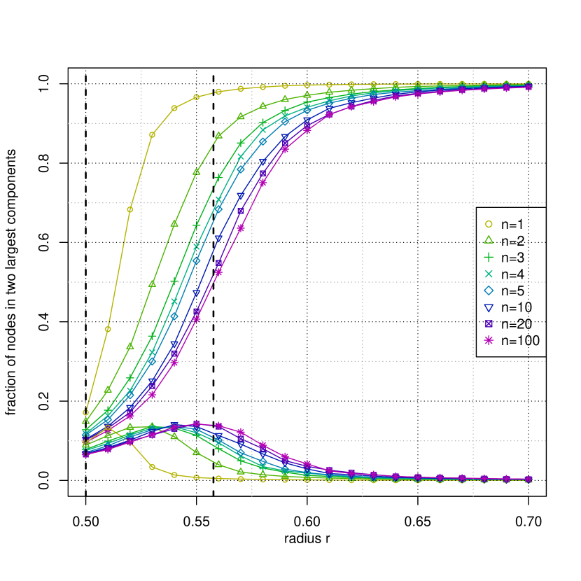
Figure 2: Mean fractions of nodes in the two largest components of the sub-Poisson Boolean model $C(\Phi^{pert}_{Bin}(n),r)$ as a function of $r$; see Section 6.1.1. The underlying pp $\Phi^{pert}_{Bin}(n)$ are $dcx$ increasing in $n$ to the Poisson pp $\Phi_{\lambda}$ of intensity $\lambda=2/(\sqrt{3})=1.154701$. The right dashed vertical line corresponds to the radius $r=0.5576495$ which is believed to be close to the critical radius $r_{c}(\Phi_{\lambda})$ for the Poisson pp. The left dashed vertical line correspond to the critical radius $r_{c}(\Phi)=0.5$ for the non-perturbed lattice.

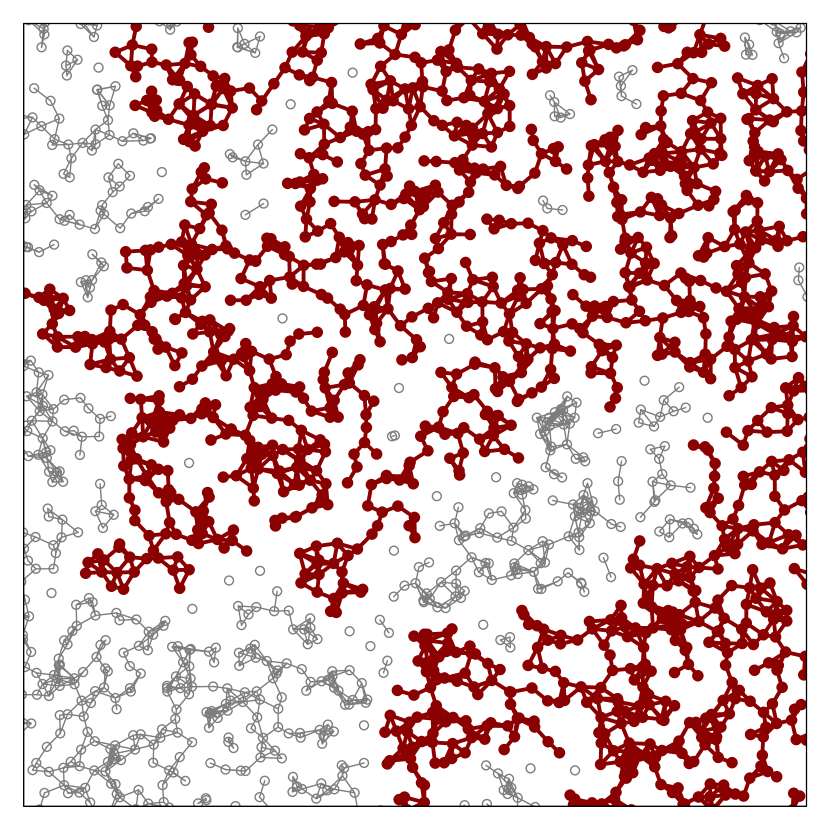
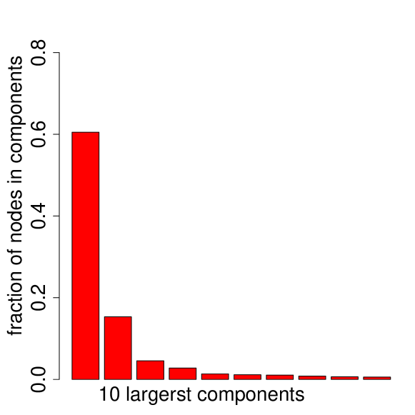
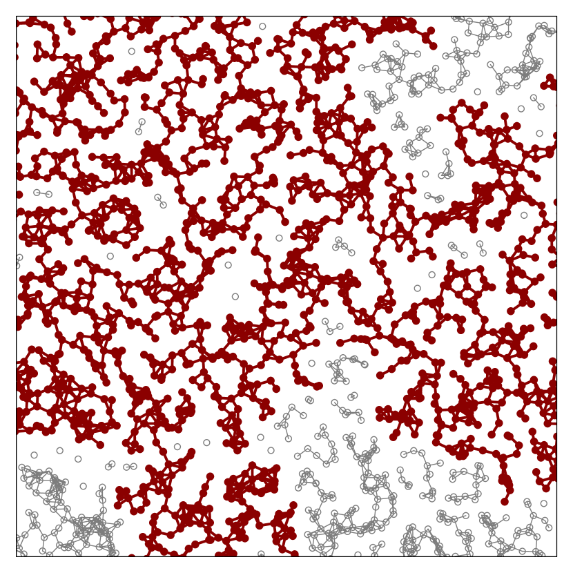
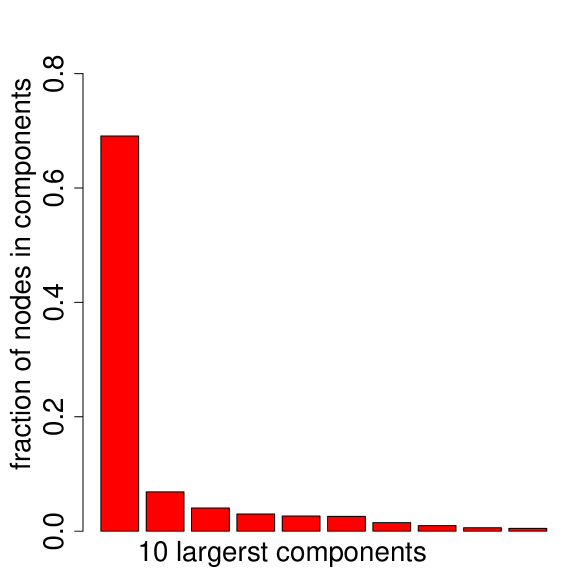
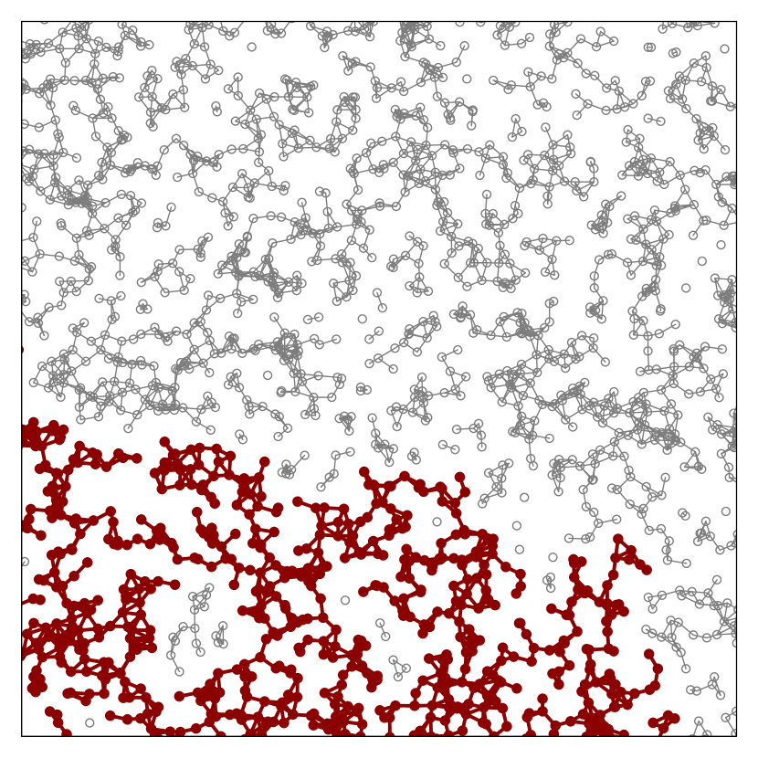
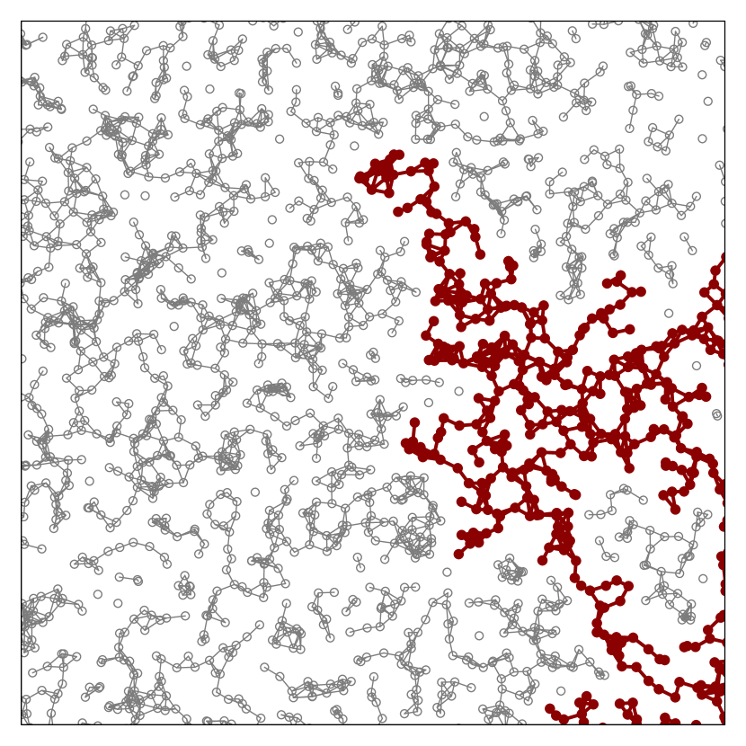
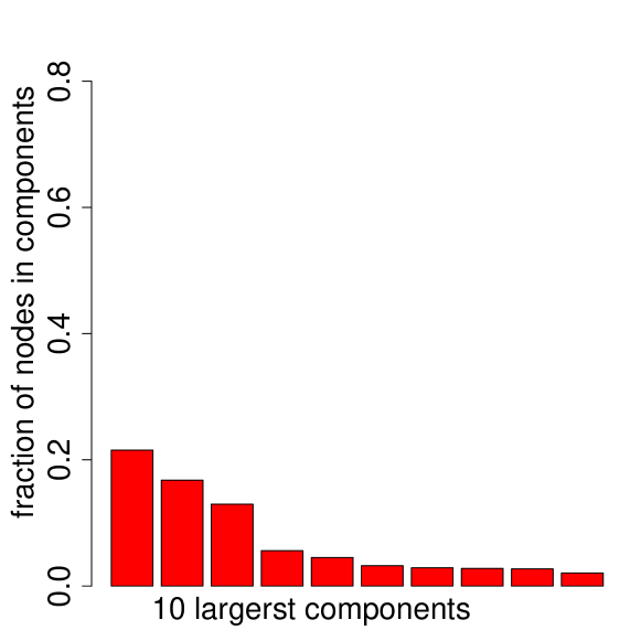
   $n=5$     $n=6$     $n=7$     $n=8$

Figure 3: Illustration of the phase transition in the clustering parameter $n$ for the sub-Poisson Boolean model $C(\Phi^{pert}_{Bin}(n),r)$ with $r=0.55$; see Section 6.1.1. The largest component in the simulation window is highlighted. Bar-plots show the fraction of nodes in ten largest components.

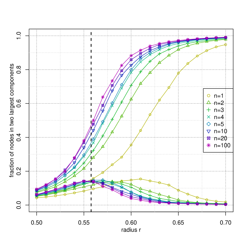
Figure 4: Mean fractions of nodes in two largest components of super-Poisson Boolean model $C(\Phi^{pert}_{N\!Bin}(n),r)$ in function of $r$; see Section 6.1.1. The underlying pp $\Phi^{pert}_{N\!Bin}(n)$ are $dcx$ decreasing in $n$ to Poisson pp $\Phi_{\lambda}$ of intensity $\lambda=2/(\sqrt{3})=1.154701$.

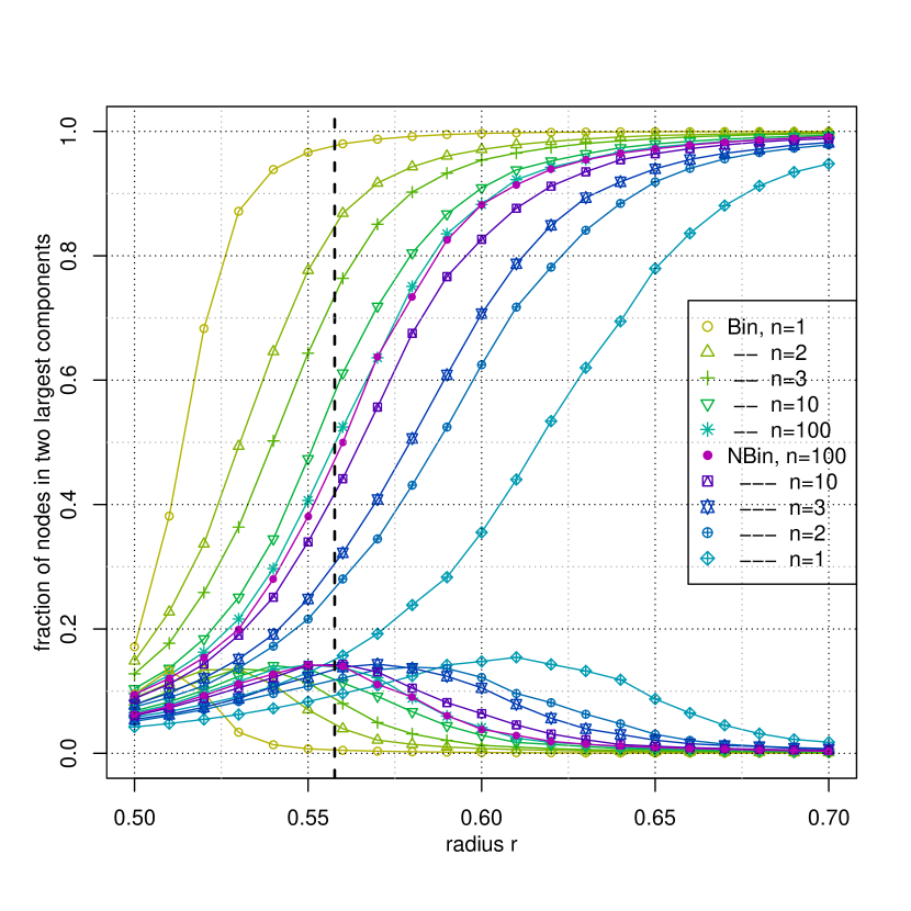
Figure 5: From sub- to super-Poisson. Figures 2 and 4 together.

Consider Boolean model $C(\Phi,r)$ with spherical grains of radius $r$. Recall that the critical radius $r_{c}=r_{c}(\Phi)$ is the smallest radius $r$ such that $C(\Phi,r)$ percolates with positive probability. In what follows, we will show some example of simulation results supporting the hypothesis that $\Phi_{1}\leq_{dcx}\Phi_{2}$ implies $r_{c}(\Phi_{1})\leq r_{c}(\Phi_{2})$.

Consider two families of $dcx$ ordered pp $\Phi^{pert}$ constructed as perturbations of the hexagonal lattice $\Phi$ (of inter-node distance 1) with node translation kernel ${\mathcal{X}}(x,\cdot)$ being uniform within the hexagonal cell of $x\in\Phi$ and different replication kernels ${\mathcal{N}}(x,\cdot)$ (see Example 6.3). Specifically, assume binomial $Bin(n,1/n)$ and negative binomial $N\!Bin(n,1/(1+n))$ distribution for ${\mathcal{N}}(x,\cdot)$ with $n\geq 1$. Recall from Example 6.3 that the former assumption leads to $dcx$ increasing in $n$ family of sub-Poisson pp $\Phi^{pert}=\Phi^{pert}_{Bin}(n)$ converging to Poisson pp (of intensity $\lambda=2/(\sqrt{3})=1.154701$) when $n\to\infty$, while the latter assumption leads to $dcx$ decreasing family of super-Poisson pp $\Phi^{pert}=\Phi^{pert}_{N\!Bin}(n)$ converging in $n$ to the same Poisson pp. The critical radius $r_{c}(\Phi_{\lambda})$ for this Poisson pp is known to be close to the value $r=0.5576495$; .

In order to get an idea about the critical radius, we have simulated 300 realizations of the Boolean model $C(\Phi^{pert},r)$ for $r$ varying from $r=0.5$ to $r=0.7$ in the square window $[0,50]^{2}$. The fraction of nodes in the two largest components in the window was calculated for each realization of the model for each $r$ and the obtained results were averaged over 300 realizations of the model. The resulting mean fractions of nodes in the two largest components as a function of $r$ are plotted on Figures 2 and 4 for binomial (sub-Poisson) and negative binomial (super-Poisson) pp, respectively. The two families are compared in Figure 5. The obtained curves support the hypothesis that the clustering of the pp of germs negatively impacts the percolation of the corresponding Boolean models. Moreover, Figure 3 illustrates what could be called the “phase transition for percolation in the clustering parameter” $n$ for $\Phi^{pert}_{Bin}(n)$.

6.2 Super-Poisson point process with a trivial percolation phase transition

The objective of this section is to show examples of highly clustered and well percolating pp. More precisely we show examples of Poisson-Poisson cluster pp of arbitrarily small intensity, which are super-Poisson, and which percolate for arbitrarily small radii.

Example 6.4.

[Poisson-Poisson cluster pp with annular clusters] Let $\Phi_{\alpha}$ be the Poisson pp of intensity $\alpha$ on the plane $\mathbb{R}^{2}$; we call it the process of cluster centers. Consider its perturbation $\Phi_{\alpha}^{R,\delta,\mu}$ (cf. Example 6.2) with the following translation and replication kernels. Let ${\mathcal{X}}(x,\cdot)$ be the uniform distribution on the annulus $B_{O}(R)\setminus B_{O}(R-\delta)$ centered at $x$ of inner and outer radii $R-\delta$ and $R$ respectively, for some $0<\delta\leq R<\infty$; see Figure 6. Let ${\mathcal{N}}(x,\cdot)$ be the Poisson distribution $Poi(\mu)$. The process $\Phi_{\alpha}^{R,\delta,\mu}$ is a Poisson-Poisson cluster pp; i.e., a Cox pp with the random intensity measure $\Lambda(\cdot):=\mu\sum_{X\in\Phi_{\alpha}}{\mathcal{X}}(x,\cdot-x)$. By [Błaszczyszyn and Yogeshwaran(2009), Proposition 5.2], it is a super-Poisson pp. More precisely, $\Phi_{\lambda}\leq_{dcx}\Phi_{\alpha}^{R,\delta,\mu}$, where $\Phi_{\lambda}$ is homogeneous Poisson pp of intensity $\lambda=\alpha\mu$.

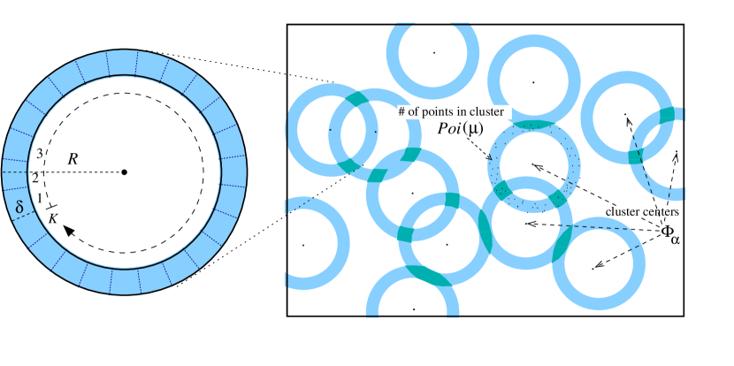
Figure 6: Poisson-Poisson cluster process of annular cluster; cf. Example 6.4.

For a given arbitrarily large intensity $\lambda<\infty$, taking sufficiently small $\alpha,R$, $\delta=R$ and sufficiently large $\mu$, it is straightforward to construct a Poisson-Poisson cluster pp $\Phi_{\alpha}^{R,R,\mu}$ with spherical clusters, which has an arbitrarily large critical radius $r_{c}$ for percolation. It is less evident that one can construct a Poisson-Poisson cluster pp that always percolates, i.e., with degenerate critical radius $r_{c}=0$.

Proposition 4.

Let $\Phi_{\alpha}^{R,\delta,\mu}$ be a Poisson-Poisson cluster pp with annular clusters on the plane $\mathbb{R}^{2}$ as in Example 6.4. Given arbitrarily small $a,r>0$, there exist constants $\alpha,\mu,\delta,R$ such that $0<\alpha,\mu,\delta,R<\infty,$ the intensity $\alpha\mu$ of $\Phi_{\alpha}^{R,\delta,\mu}$ is equal to $a$ and the critical radius for percolation $r_{c}(\Phi_{\alpha}^{R,\delta,\mu})\leq r$. Moreover, for any $a>0$ there exists pp $\Phi$ of intensity $a$, which is $dcx$-larger than the Poisson pp of intensity $a$, and which percolates for any $r>0$; i.e., $r_{c}(\Phi)=0$.

Proof 6.5.

Let $a,r>0$ be given. Assume $\delta=r/2$. We will show that there exist sufficiently large $\mu,R$ such that $r_{c}(\Phi_{\alpha}^{R,\delta,\mu})\leq r$ where $\alpha=a/\mu$. In this regard, denote $K:=2\pi R/r$ and assume that $R$ is chosen such that $K$ is an integer. For a $\alpha>0$ and any point (cluster center) $X_{i}\in\Phi_{\alpha},$ let us partition the annular support $A_{X_{i}}(R,\delta):=B_{X_{i}}(R)\setminus B_{X_{i}}(R-\delta)$ of the translation kernel $X_{i}+{\mathcal{X}}(X_{i},\cdot)$ (support of the Poisson pp constituting the cluster centered at $X_{i}$) into $K$ cells as shown in Figure 6. We will call $X_{i}$ “open” if in each of the $K$ cells of $A_{X_{i}}(R,\delta),$ there exists at least one replication of the point $X_{i}$ among the Poisson $Poi(\mu)$ (with $\alpha=a/\mu$) number of total replications of the point $X_{i}$. Note that given $\Phi_{\alpha}$, each point $X_{i}\in\Phi_{\alpha}$ is open with probability $p(R,\mu):=(1-e^{-\mu/K})^{K}$, independently of other points of $\Phi_{\alpha}$. Consequently, open points of $\Phi_{\alpha}$ form a Poisson pp of intensity $\alpha p(R,\mu)$; call it $\Phi_{open}$. Note that the maximal distance between any two points in two neighbouring cells of the same cluster is not larger than $2(\delta+2\pi R/K)=2r$. Similarly, the maximal distance between any two points in two non-disjoint cells of two different clusters is not larger than $2(\delta+2\pi R/K)=2r$. Consequently, if the Boolean model $C(\Phi_{open},A_{0}(R,\delta))$ with annular grains percolates then the Boolean model $C(\Phi_{\alpha}^{R,\delta,\mu},r)$ with spherical grains of radius $r$ percolates as well. The former Boolean model percolates if and only if $C(\Phi_{open},B_{0}(R))$ percolates. Hence, in order to guarantee $r_{c}(\Phi_{\alpha}^{R,\delta,\mu})\leq r,$ it is enough to chose $R,\mu$ such that the volume fraction $1-e^{-\alpha p(R,\mu)\pi R^{2}}=1-e^{-ap(R,\mu)\pi R^{2}/\mu}$ is larger than the critical volume fraction for the percolation of the spherical Boolean model on the plane. In what follows, we will show that by choosing appropriate $R,\mu$ one can make $p(R,\mu)R^{2}/\mu$ arbitrarily large. Indeed, take

$$\mu:=\mu(R)=\frac{2\pi R}{r}\log{\frac{R}{\sqrt{\log R}}}=\frac{2\pi R}{r}\Bigl{(}\log R-\frac{1}{2}\log\log R\Bigr{)}\,.$$

Then, as $R\to\infty$

$$p(R,\mu)R^{2}/\mu = \frac{R^{2}}{\mu}(1-e^{-\mu r/(2\pi R)})^{2\pi R/r}$$

$$= \frac{Rr}{2\pi(\log R-\frac{1}{2}\log\log R)}\Bigl{(}1-\frac{\sqrt{\log R}}{R}\Bigr{)}^{2\pi R/r}$$

$$= e^{O(1)+\log R-\log(2\pi(\log R-\frac{1}{2}\log\log R))-O(1)\sqrt{\log R}}\to\infty\,.$$

This completes the proof of the first statement.

In order to prove the second statement, for a given $a>0$, denote $a_{n}:=a/2^{n}$ and let $r_{n}=1/n$. Consider a sequence of independent (super-Poisson) Poisson-Poisson cluster pp $\Phi_{n}=\Phi_{\alpha_{n}}^{R_{n},\delta_{n},\mu_{n}}$ with intensities $\lambda_{n}:=\alpha_{n}\mu_{n}=a_{n}$, satisfying $r_{c}(\Phi_{n})\leq r_{n}$. The existence of such pp was shown in the first part of the proof. By the fact that $\Phi_{n}$ are super-Poisson for all $n\geq 0$ and by [Błaszczyszyn and Yogeshwaran(2009), Proposition 3.2(4)] the superposition $\Phi=\bigcup_{n=1}^{\infty}\Phi_{n}$ is $dcx$-larger than Poisson pp of intensity $a$. Obviously $r_{c}(\Phi)=0$. This completes the proof of the second statement.

Remark 5.

By Proposition 4 we know that there exists pp $\Phi$ with intensity $a>0$, such that $r_{c}(\Phi)=0$ and $\Phi_{a}\leq_{dcx}\Phi$, where $\Phi_{a}$ is homogeneous Poisson pp. Since one knows that $r_{c}(\Phi_{a})>0$ so $\Phi$ is a counterexample for the monotonicity of $r_{c}$ in $dcx$ ordering of pp.

6.3 Determinantal and permanental point processes

In this section, we will give some results related to the $dcx$ comparison of determinantal and permanental pp with respect to the Poisson pp. Refer to [Ben Hough et al.(2006)Ben Hough, Krishnapur, Peres, and Virág] for a quick introduction to these pp and for a more elaborate reading, see [Ben Hough et al.(2009)Ben Hough, Krishnapur, Peres, and Virág]. To this end, we will now recall a general framework (see [Ben Hough et al.(2009)Ben Hough, Krishnapur, Peres, and Virág, Chapter 4]) which allows us to study ordering of determinantal and permanental pp more explicitly.

6.3.1 Integral kernels

Let $K:\mathbb{R}^{d}\times\mathbb{R}^{d}\to\mathbb{C}$ (where $\mathbb{C}$ are complex numbers) be a locally square-integrable kernel, with respect to $\mu^{\otimes 2}$ on $\mathbb{R}^{2d}$ . Then $K$ defines an associated integral operator $\mathcal{K}_{D}$ on $L^{2}(D,\mu)$ as $\mathcal{K}_{D}f(x)=\int_{D}K(x,y)f(y)\,\mu(dy)$ for complex-valued, square-integrable $f$ on $D$ ($f\in L^{2}(D,\mu)$). This operator is compact and hence its spectrum is discrete. The only possible accumulation point is $0$ and every non-zero eigenvalue has finite multiplicity. Assume moreover that for each compact $D$ the operator $\mathcal{K}_{D}$ is Hermitian , positive semi-definite , and trace-class; i.e., $\sum_{j}|\lambda_{j}^{D}|<\infty$, where $\lambda_{j}^{D}$ denote the eigenvalues of $\mathcal{K}_{D}$. By the positive semi-definiteness of $\mathcal{K}_{D},$ these eigenvalues are non-negative. Further, one can show (cf. [Ben Hough et al.(2009)Ben Hough, Krishnapur, Peres, and Virág, Lemma 4.2.2]) that for each compact $D$, there exists a “version” $K_{D}(x,y)$ of the kernel $K$, defined on $D^{\prime}\subset D$ such that $\mu(D\setminus D^{\prime})=0$, having the same associated operator $\mathcal{K}_{D}$ on $L^{2}(D,\mu)$  , which is Hermitian and positive semi-definite. Specifically one can take $K_{D}(x,y)=\sum_{j}\lambda_{j}^{D}\phi_{j}^{D}(x)\overline{\phi_{j}^{D}(y)}$ where $\phi_{j}^{D}(\cdot)$ are the corresponding normalized eigenfunctions of $\mathcal{K}_{D}$.

Example 6.6.

Determinantal pp. A simple pp on $\mathbb{R}^{d}$ is said to be a determinantal pp with a kernel $K(x,y)$ with respect to a Radon measure $\mu$ on $\mathbb{R}^{d}$ if the joint intensities of the pp with respect to the $k\,$th-order product $\mu^{\otimes k}$ of $\mu$ satisfy $\rho^{(k)}(x_{1},\ldots,x_{k})=\det\big{(}K(x_{i},x_{j})\big{)}_{1\leq i,j\leq k}$ for all $k$, where $\big{(}a_{ij}\big{)}_{1\leq i,j\leq k}$ stands for a matrix with entries $a_{ij}$ and $\det\big{(}\cdot\big{)}$ denotes the determinant of the matrix. Note that the mean measure of the determinantal pp (if it exists) is equal to $\alpha(\cdot)=\int_{\cdot}K(x,x)\,\mu(dx)$. Clearly, one needs assumptions on the kernel $K(x,y)$ for the above equation to define the joint intensities of a pp. In what follows, we shall assume that the kernel $K$ is an integral kernel satisfying the assumptions of Section 6.3.1. Then, there exists a unique pp $\Phi^{det}$ on $\mathbb{R}^{d}$, such that for each compact $D$, the restriction of $\Phi^{det}$ to $D$ is a determinantal pp with kernel $K_{D}$ if and only if the eigenvalues of $\mathcal{K}_{D}$ are in $[0,1]$. This latter condition is equivalent to $\lambda_{j}^{D}\in[0,1]$ for all compact $D$; cf. [Ben Hough et al.(2009)Ben Hough, Krishnapur, Peres, and Virág, Theorem 4.5.5]. We will call this pp determinantal pp with the trace-class integral kernel $K(x,y)$.

Example 6.7.

Permanental pp. Similar to determinantal pp, one says that a simple pp is a permanental pp with a kernel $K(x,y)$ with respect to a Radon measure $\mu$ on $\mathbb{R}^{d}$ if the joint intensities of the pp with respect to $\mu^{\otimes k}$ satisfy $\rho^{(k)}(x_{1},\ldots,x_{k})=\text{per}\big{(}K(x_{i},x_{j})\big{)}_{1\leq i,j\leq k}$ for all $k$, where $\text{per}\big{(}\cdot\big{)}$ stands for the permanent of a matrix. Note that the mean measure of the permanental pp is also equal to $\alpha(\cdot)=\int_{.}K(x,x)\,\mu(dx)$. Again, will assume that $K(x,y)$ is an integral kernel as in Section 6.3.1. Then, there exists a unique pp $\Phi^{perm}$ on $\mathbb{R}^{d}$, such that for each compact $D$, the restriction of $\Phi^{perm}$ to $D$ is a permanental pp with kernel $K_{D}$; cf. [Ben Hough et al.(2009)Ben Hough, Krishnapur, Peres, and Virág, Corollary 4.9.9]. We will call this pp permanental pp with the trace-class integral kernel $K(x,y)$. From [Ben Hough et al.(2006)Ben Hough, Krishnapur, Peres, and Virág, Proposition. 35 and Remark 36], we also know that $\Phi^{perm}$ is a Cox pp with intensity field $|F|^{2},$ where $F$ is some complex Gaussian process on $\mathbb{R}^{d}$.

The following properties hold true for determinantal and permanental pp with a trace-class integral kernel $K(x,y)$.

• $\Phi^{det}$ is $\alpha$-weakly sub-Poisson, while $\Phi^{perm}$ is $\alpha$-weakly super-Poisson; both comparable with respect to the Poisson pp with mean measure $\alpha(\cdot)$ given by $\alpha(D)=\int_{D}K_{D}(x,x)\,\mu(d)=\sum_{j}\lambda_{j}^{D}$, where the summation is taken over all the eigenvalues $\lambda_{j}^{D}$ of $\mathcal{K}_{D}$. The proof follows by the fact that $K_{D}(x,y)$ is Hermitian and positive semi-definite. Hence, by the Hadamard’s inequality, $0\leq\det\big{(}K_{D}(x_{i},x_{j})\big{)}_{1\leq i,j\leq k}\leq\prod_{i=1}^{k}K_{D}(x_{i},x_{i})$ which implies (3). For $\Phi^{perm}$, the proof follows from the permanent analogue of the Hadamard’s inequality (see [Marvin(1964)]). In fact, for the above comparison to be true it suffices for the kernel $K(x,y)$ to be Hermitian and positive semi-definite.

• It is known that for each compact $D$, $\Phi^{det}(D)$ has the same distribution as the sum of independent Bernoulli random variables $Bin(1,\lambda_{j}^{D})$ cf. [Ben Hough et al.(2009)Ben Hough, Krishnapur, Peres, and Virág, Theorem 4.5.3], while $\Phi^{perm}(D)$ has the same distribution as the sum of independent geometric random variables $Geo(1/(1+\lambda_{j}^{D}))$, where the summation is taken over all eigenvalues $\lambda_{j}^{D}$ of $\mathcal{K}_{D}$; cf. [Ben Hough et al.(2009)Ben Hough, Krishnapur, Peres, and Virág, Theorems 4.5.3 and 4.9.4]. Consequently

  $$\Phi^{det}(D)\leq_{cx}Poi(\sum_{j}\lambda_{j}^{D})\leq_{cx}\Phi^{perm}(D)\,,$$ (21)

  with the left inequality holding provided $\Phi^{det}$ exists (i.e.; $\lambda_{j}^{D}\in[0,1]$ for all compact $D$).

• Inequalities (21) imply that $\Phi^{det}$ is $\nu$-weakly sub-Poisson, while $\Phi^{perm}$ is $\nu$-weakly super-Poisson. Consequently, $\Phi^{det}$ is weakly sub-Poisson, while $\Phi^{perm}$ is weakly super-Poisson.

In Proposition 6, we will strengthen (21) proving $dcx$ ordering of finite-dimensional distributions of $\Phi^{det}$ and $\Phi^{perm}$ on mutually disjoint simultaneously observable sets $D_{1},\ldots,D_{k}$. Simultaneous observability means that the eigenfunctions of $\mathcal{K}_{\bigcup D_{i}}$, restricted to $D_{i}$ are also eigenfunctions of $\mathcal{K}_{D_{i}}$ for every $i=1,\ldots,k$.

Proposition 6.

Let $\Phi^{det}$ and $\Phi^{per}$ be, respectively, the determinantal and permanental pp with a trace-class integral kernel $K$ and with $\Phi^{det}$ being defined only if the spectrum of $\mathcal{K}_{\mathbb{R}^{d}}$ is in $[0,1]$. Denote by $\Phi^{Poi}$ the Poisson pp of mean measure $\alpha(\cdot)$ given by $\alpha(D)=\sum_{j}\lambda_{j}^{D}$ for all compact $D$, where the summation is taken over all eigenvalues $\lambda_{j}^{D}$ of $\mathcal{K}_{D}$. Let $D_{1},\ldots,D_{k}$ be mutually disjoint, simultaneously observable (with respect to the kernel $K$) compact subsets of $\mathbb{R}^{d}$ and $D=\bigcup D_{i}$. Then

$$\Bigl{(}\Phi^{det}(D_{1}),\ldots,\Phi^{det}(D_{k})\Bigr{)} \leq_{dcx} \Bigl{(}\Phi^{Poi}(D_{1}),\ldots,\Phi^{Poi}(D_{k})\Bigr{)}$$

$$\leq_{dcx} \Bigl{(}\Phi^{per}(D_{1}),\ldots,\Phi^{per}(D_{k})\Bigr{)}\,.$$

Proof 6.8.

From [Ben Hough et al.(2009)Ben Hough, Krishnapur, Peres, and Virág, Prop. 4.5.9], we know that

$$\Bigl{(}\Phi^{det}(D_{1}),\ldots,\Phi^{det}(D_{k})\Bigr{)}\stackrel{{\scriptstyle d}}{{=}}\sum_{j=1}^{J}\boldsymbol{\xi}_{j},$$

with $J$ denoting the number of eigenvalues of $\mathcal{K}_{D}$ ($J=\infty$ and $0$ allowed and in the latter case the sum is understood as $0$) and $\boldsymbol{\xi}_{j}$, $j=1,\ldots,J$ are are independent vectors, with components $\boldsymbol{\xi}_{j}=(\xi_{j,1},\ldots,\xi_{j,k})$ whose distributions are $\mathsf{P}\left(\xi_{j,l}=0\;\text{for all}\;\allowbreak l\not=i,\xi_{j,i}=1\right)=\lambda^{D}_{j,i}$ and $\mathsf{P}(\xi_{j,l}=0\;\text{for}\allowbreak\;\text{all}\;l=1,\ldots,k)=1-\lambda^{D}_{j}$, where $\{\lambda_{j,i}\}_{j=1,\ldots,J}$ are the eigenvalues of $\mathcal{K}_{D_{i}}$ and $\lambda^{D}_{j}=\sum_{i=1}^{k}\lambda^{D}_{j,i}$, $j=1,\ldots,J$ are the eigenvalues of $\mathcal{K}_{D}$. Due to the independence of $\boldsymbol{\xi_{j}}$’s and the assumption $\sum_{j=1}^{J}\lambda_{j}<\infty$ (local trace-class property of $\mathcal{K}_{D}$), it is enough to prove for each $j$, that $\boldsymbol{\xi}_{j}\leq_{dcx}\boldsymbol{\zeta}_{j}$ where $\boldsymbol{\zeta}_{j}=(\zeta_{j,1},\ldots,\zeta_{j,k})$ is the vector of independent Poisson random variables $\zeta_{j,l}\sim Poi(\lambda^{D}_{j,l})$. In this regard, note that the random vectors $\boldsymbol{\xi}_{j}$ and $\boldsymbol{\zeta}_{j}$ can be coupled as follows: $\boldsymbol{\xi}_{j}=\sum_{i=1}^{N}\boldsymbol{\xi}^{\prime}_{i}$, $\boldsymbol{\zeta}_{j}=\sum_{i=1}^{M}\boldsymbol{\xi}^{\prime}_{i}$ where $N\sim Bin(1,\lambda^{D}_{j})$, $M\sim Poi(\lambda^{D}_{j})$ and given $N,M$, $\boldsymbol{\xi}^{\prime}_{i}$, $i\geq 1$ are independent multinomial vectors $Mul(1,\lambda^{D}_{j,1}/\lambda^{D}_{j},\ldots,\lambda^{D}_{j,k}/\lambda^{D}_{j})$ . Then, $\boldsymbol{\xi}_{j}\leq_{dcx}\boldsymbol{\zeta}_{j}$ follows from the fact that $Bin(1,p)\leq_{cx}Poi(p)$ (see Example 6.3) and Lemmas 1, 2. This completes the proof of the inequality for the determinantal pp.

Regarding the permanental pp, we know from [Ben Hough et al.(2009)Ben Hough, Krishnapur, Peres, and Virág, Theorem 4.9.7] that the distribution of

$$\Bigl{(}\Phi^{per}(D_{1}),\ldots,\Phi^{per}(D_{k})\Bigr{)}\stackrel{{\scriptstyle d}}{{=}}\sum_{j=1}^{J}\boldsymbol{\eta}_{j},$$

where $\boldsymbol{\eta}_{j}$, $j=1,\ldots,J$ are are independent vectors, with $\boldsymbol{\eta}_{j}=\sum_{i=1}^{K}\boldsymbol{\xi}^{\prime}_{i}$, where $K\sim Geo(1/(1+\lambda^{D}_{j})$ and, given $K$, independent multinomial vectors $\boldsymbol{\xi}^{\prime}_{i}$, $i=1,\ldots$ as above. Similarly, as for the determinantal pp, the required inequality follows from the ordering, $\boldsymbol{\zeta}_{j}\leq_{dcx}\boldsymbol{\eta}_{j}$ for all $j$, which follows from the fact that $Poi(\lambda)\leq_{cx}Geo(1/(1+\lambda)$ (see Example 6.3) and Lemmas 1, 2. This completes the proof.

Remark 7.

Note that the key observation used in the above proof is that the number of points in disjoint, simultaneously observable sets $D_{1},\ldots,D_{k}$ can be represented as a sum of independent vectors, which themselves are binomial (for determinantal) or Poisson (for Poisson) or geometric (for permanental) sums of some further independent vectors. This is exactly the same representation as for the perturbed pp of Section 6.1 (available for any disjoint sets $B_{1},\ldots,B_{k}$); cf the proof of Proposition 1. In both cases, this representation and Lemmas 1, 2 allow us to conclude $dcx$ ordering of the corresponding vectors.

Example 6.9.

Ginibre process. Let $\Phi^{G}$ be the determinantal pp on $\mathbb{R}^{2}$ with kernel $K((x_{1},x_{2}),(y_{1},y_{2}))=\exp[(x_{1}y_{1}+x_{2}y_{2})+i(x_{2}y_{1}-x_{1}y_{2})]$, $x_{j},y_{j}\in\mathbb{R}$, $j=1,2$, with respect to the measure $\mu(d(x_{1},x_{2}))=\pi^{-1}\exp[-x_{1}^{2}-x_{2}^{2}]\,dx_{1}dx_{2}$. This process is known as the infinite Ginibre pp. Denote by $\Psi^{G}=\{|X_{i}|^{2}:X_{i}\in\Phi^{G}\},$ the pp on $\mathbb{R}^{+}$ of the squared radii of the points of $\Phi^{G}$. We know that an arbitrary finite collection of the annuli centered at the origin $D_{i}=\{(x_{1},x_{2}):r_{i}\leq x_{1}^{2}+x_{2}^{2}\leq R_{i}\}$ is simultaneously observable for this pp; cf. [Ben Hough et al.(2009)Ben Hough, Krishnapur, Peres, and Virág, Example 4.5.8]. Using this observation, Proposition 6 and the fact that $dcx$ order of pp on $\mathbb{R}$ is generated by the semi-ring of intervals, we conclude that $\Psi^{G}$ is $dcx$ smaller than the Poisson pp $\Phi^{1}$ of unit intensity on $\mathbb{R}^{+}$. A partial result, $\Psi^{G}([0,r])\leq_{cx}\Phi^{1}([0,r])$ for all $r\geq 0$, was proved in [Błaszczyszyn and Yogeshwaran(2009)].

7 Concluding remarks

We come back to the initial heuristic discussed in the Introduction — clustering in a point process should increase the critical radius for the percolation of the corresponding continuum percolation model. As we have seen, even a relatively strong tool such as the $dcx$ order falls short, when it comes to making a formal statement of this heuristic.

The two natural questions are what would be a more suitable measure of clustering that can be used to affirm the heuristic and whether $dcx$ order can satisfy a weaker version of the conjecture.

As regards the first question, one might start by looking at other dependence orders such as super-modular, component-wise convex or convex order but it has been already shown that the super-modular and component-wise convex orders are not suited to comparison of clustering in point processes (cf. [Yogeshwaran(2010), Section 4.4]). Properties of convex order on point processes are yet to be investigated fully and this research direction is interesting in its own right, apart from its relation to the above conjecture. In a similar vein, it is of potential interest to study other stochastic orders on point processes.

On the second question, it is pertinent to note that sub-Poisson point processes surprisingly exhibited non-trivial phase transitions for percolation. Such well-behavedness of the sub-Poisson point processes makes us wonder if it is possible to prove a rephrased conjecture saying that any homogeneous sub-Poisson pp has a smaller critical radius for percolation than the Poisson pp of the same intensity. Such a conjecture matches well with [Benjamini and Stauffer(2011), Conjecture 4.6].

Appendix A

The following result, similar to [Meester and Shanthikumar(1993), Lemma 2.17] is used in the proof of Propositions 1 and 6.

Lemma 1.

Let ${\boldsymbol{\xi}}_{i}=(\xi_{i}^{1},\ldots,\xi_{i}^{k})\in\mathbb{R}^{k}$, ($i=1,2,\ldots$) be independent, identically distributed vectors of (possibly dependent) non-negative random variables. Suppose $f$ is a $dcx$ function on $\mathbb{R}^{k}$. Then, the function $g$ defined on $\mathbb{Z}$ by $g(n)=\mathsf{E}\!\left(f(\text{sgn}(n)\sum_{i=1}^{|n|}{\boldsymbol{\xi}}_{i})\right)$ for $n\not=0$ and $g(0)=0$ is convex on $\mathbb{Z}$.

Proof A.1.

We will prove that $g(n)$ has non-negative second differences

$$g(n-1)+g(n+1)-2g(n)\geq 0\qquad\text{for all $n\in\mathbb{Z}$}$$ (22)

and use the first part of Lemma 2. To prove (22), define $G(n,m):=\sum_{i=n+1}^{m}{\boldsymbol{\xi}}_{i}$ for $0\leq n<m$ and $G(n,n):=(0,0,\ldots,0)\in\mathbb{R}^{k}$ for $n\geq 0$. We have for $n\geq 1$,

$$2g(n) = 2\mathsf{E}\!\left(f\Bigl{(}G(0,n)\Bigr{)}\right)$$

$$= \mathsf{E}\!\left(f\Bigl{(}G(0,n-1)+G(n-1,n)\Bigr{)}\right)+\mathsf{E}\!\left(f\Bigl{(}G(0,n)\Bigr{)}\right)$$

$$= \mathsf{E}\!\left(f\Bigl{(}G(0,n-1)+G(n,n+1\Bigr{)}\right)+\mathsf{E}\!\left(f\Bigl{(}G(0,n)\Bigr{)}\right)$$

$$= \mathsf{E}\!\left(f\Bigl{(}G(0,n-1)+G(n,n+1\Bigr{)}+f\Bigl{(}G(0,n)\Bigr{)}\right)$$

$$\leq \mathsf{E}\!\left(f\Bigl{(}G(0,n-1)\Bigr{)}+f\Bigl{(}G(0,n)+G(n,n+1)\Bigr{)}\right)$$

$$= g(n-1)+g(n+1)\,,$$

where for the third equality we have used mutual independence of $G(0,n-1),G(n-1,n),G(n,n+1)$ and the fact that $G(n-1,n)$ and $G(n,n+1)$ have the same distribution, while the inequality follows from the $dcx$ property of $f$ and the assumption ${\boldsymbol{\xi}}_{i}\geq 0$. This proves (22) for $n\geq 1$. Similar reasoning allows to show (22) for $n\leq-1$. Finally, note that for $n=0$

$$2g(0) = 2f\Bigl{(}(0,\ldots,0)\Bigr{)}$$

$$= \mathsf{E}\!\left(f\Bigl{(}-G(0,1)+G(0,1)\Bigr{)}+f\Bigl{(}(0,\ldots,0)\Bigr{)}\right)$$

$$\leq \mathsf{E}\!\left(f\Bigl{(}-G(0,1)\Bigr{)}+f\Bigl{(}G(0,1)\Bigr{)}\right)$$

$$= g(-1)+g(1)\,,$$

We will prove the following two technical results regarding convex functions. We were not able to find their proofs in the literature.

Lemma 2.

Let $g(n)$ be a real valued function defined for all integer $n\in\mathbb{Z}$ and satisfying condition (22). Then the following two statements are true:

1. For all $n\geq 2$

   $$g\Bigl{(}\sum_{i=1}^{n}\lambda_{i}k_{i}\Bigr{)} \leq \sum_{i=1}^{n}\lambda_{i}g(k_{i})$$ (23)

   for all $$k_{i}\in\mathbb{Z} 0\leq\lambda_{i}\leq 1 \sum_{i=1}^{n}\lambda_{i}=1 \sum_{i=1}^{n}\lambda_{i}k_{i}\in\mathbb{Z}$$ and , such that .

2. Function $g(\cdot)$ can be extended to a real valued convex function defined on real numbers $\mathbb{R}$.

Proof A.2.

Ad 1. As mentioned in [Marshall et al.(2009)Marshall, Olkin, and Arnold, Section V.16.B.10.a] it is easy to see that (22) is equivalent to (23) with $n=2$. Assume now that (23) holds true for some $n\geq 2$ (and all $0\leq\lambda_{i}\leq 1$, $k_{i}\in\mathbb{Z}$, $i=1,\ldots,n$ satisfying $\sum_{i=1}^{n}\lambda_{i}=1$, $\sum_{i=1}^{n}\lambda_{i}k_{i}\in\mathbb{Z}$). We will prove that it holds true for $n+1$ as well. In this regard, define for a given $k\in\mathbb{Z}$ and distinct (otherwise we use directly the inductive assumption) $k_{1},\ldots,k_{n+1}\in\mathbb{Z}$, the following functions:

$$\lambda_{n}=\lambda_{n}(\lambda_{1},\ldots,\lambda_{n-1}) := \frac{k-k_{n+1}-\sum_{i=1}^{n-1}\lambda_{i}(k_{i}-k_{n+1})}{k_{n}-k_{n+1}}$$

$$\lambda_{n+1}=\lambda_{n+1}(\lambda_{1},\ldots,\lambda_{n-1}) := 1-\sum_{i=1}^{n-1}\lambda_{i}-\lambda_{n}(\lambda_{1},\ldots,\lambda_{n-1})$$

$$F(\lambda_{1},\ldots,\lambda_{n-1}) := \sum_{i=1}^{n-1}\lambda_{i}g(k_{i})+\lambda_{n}(\lambda_{1},\ldots,\lambda_{n-1})g(k_{n})$$

$$\hskip 50.00008pt+\lambda_{n+1}(\lambda_{1},\ldots,\lambda_{n-1})g(k_{n+1})\,.$$

Note that for any $\lambda_{1},\ldots,\lambda_{n-1}$ we have $\sum_{i=1}^{n+1}\lambda_{i}=1$ and $\sum_{i=1}^{n+1}\lambda_{i}k_{i}=k$. Consider the following subset of the $n-1$-dimensional unit cube

$$C:=\Bigl{\{}(\lambda_{1},\ldots,\lambda_{n-1})\in[0,1]^{n-1}:0\leq\lambda_{n}\leq 1,0\leq\lambda_{n+1}\leq 1\Bigr{\}}\,.$$

The proof of the inductive step will be completed if we show that $F(\cdot)\geq g(k)$ on $C$. In this regard note that $C$ is closed and convex. Assume moreover that $C$ is not empty; otherwise the condition (23) is trivially satisfied. Note also that $F(\cdot)$ is an affine, real valued function defined on $\mathbb{R}^{n-1}$. Hence, by the maximum principle, the affine (hence convex) function $-F$ attains its maximum relative to $C$ on some point $(\lambda_{1}^{0},\ldots,\lambda_{n-1}^{0})\in\partial C$ of the boundary of $C$. Consequently, we have $F(\cdot)\geq F(\lambda_{1}^{0},\ldots,\lambda_{n-1}^{0})$ on $C$ and the proof of the inductive step will be completed if we show that $F(\lambda_{1}^{0},\ldots,\lambda_{n-1}^{0})\geq g(k)$. In this regard, denote $\lambda_{n}^{0}=\lambda_{n}(\lambda_{1}^{0},\ldots,\lambda_{n-1}^{0})$ and $\lambda_{n+1}^{0}=\lambda_{n+1}(\lambda_{1}^{0},\ldots,\lambda_{n-1}^{0})$. Using the continuity of the functions $\lambda_{n}(\cdot)$ and $\lambda_{n+1}(\cdot)$ is not difficult to verify that $(\lambda_{1}^{0},\ldots,\lambda_{n-1}^{0})\in\partial C$ implies $\lambda_{j}^{0}=0$ for some $j=1,\ldots,n+1$. Thus, by our inductive assumption, $F(\lambda_{1}^{0},\ldots,\lambda_{n-1}^{0})=\sum_{i=1,i\not=j}^{n+1}\lambda_{i}^{0}g(k_{i})\geq g(k)$, which completes the proof of (23) for all $n\geq 2$.

Ad 2. We will recall the arguments used in [Yan(1997)] to show that a function satisfying (23) for all $n\geq 2$ (called globally convex function there) has a convex extension on $\mathbb{R}$. In this regard, consider the epigraph $\text{epi}(g):=\{(k,\mu)\in\mathbb{Z}\times\mathbb{R}:\mu\geq g(k)\}$ of $g$ and its convex envelope $\text{epi}^{co}(g)$. It is easy to see that $\text{epi}^{co}(g)=\{(x,\mu)\in\mathbb{R}^{2}:\mu\geq\sum_{i=1}^{n}\lambda_{i}g(k_{i})$ for some $k_{i}\in\mathbb{Z}$, $0\leq\lambda_{i}\leq 1$, $\sum_{i=1}^{n}\lambda_{i}=1$ and $\sum_{i=1}^{n}\lambda_{i}k_{i}=x\}$. Define $\tilde{g}(x):=\inf\{\mu:(x,\mu)\in\text{epi}^{co}(g)\}$ for all $x\in\mathbb{R}$. The convexity of $\text{epi}^{co}(g)$ implies that $\tilde{g}$ is convex on $\mathbb{R}$ and the global convexity (23) of $g$ implies that $\tilde{g}$ is an extension of $g$. This completes the proof.

References

- [Baccelli and Błaszczyszyn(2001)] F. Baccelli and B. Błaszczyszyn. On a coverage process ranging from the Boolean model to the Poisson Voronoi tessellation, with applications to wireless communications. Adv. in Appl. Probab. (SGSA), 33:293–323, 2001.
- [Balister and Bollobás(2007)] P. Balister and B. Bollobás. Counting regions with bounded surface area. Commun. Math. Phys., 273:305–315, 2007.
- [Balister et al.(2005)Balister, Bollobás, and Walters] P. Balister, B. Bollobás, and M. Walters. Continuum percolation with steps in the square or the disc. Random Structures & Algorithms, 26(4):392––403, 2005.
- [Ben Hough et al.(2006)Ben Hough, Krishnapur, Peres, and Virág] J. Ben Hough, M. Krishnapur, Y. Peres, and B. Virág. Determinantal processes and independence. Probability Surveys, 3:206–??229, 2006.
- [Ben Hough et al.(2009)Ben Hough, Krishnapur, Peres, and Virág] J. Ben Hough, M. Krishnapur, Y. Peres, and B. Virág. Zeros of Gaussian analytic functions and determinantal point processes, volume 51. American Mathematical Society, 2009.
- [Benjamini and Stauffer(2011)] I. Benjamini and A. Stauffer. Perturbing the hexagonal circle packing: a percolation perspective. arXiv:1104.0762, 2011. URL http://arxiv.org/abs/1104.0762.
- [Błaszczyszyn and Yogeshwaran(2009)] B. Błaszczyszyn and D. Yogeshwaran. Directionally convex ordering of random measures, shot-noise fields and some applications to wireless networks. Adv. Appl. Probab., 41:623–646, 2009.
- [Błaszczyszyn and Yogeshwaran(2010)] B. Błaszczyszyn and D. Yogeshwaran. Connectivity in sub-Poisson networks. In Proc. of 48 th Annual Allerton Conference, University of Illinois at Urbana-Champaign, IL, USA, 2010.
- [Burton and Waymire(1985)] Robert Burton and Ed Waymire. Scaling limits for associated random measures. Ann. Appl. Probab., 13(4):1267–1278, 1985.
- [Daley and Vere-Jones(2007)] D. J. Daley and D. Vere-Jones. An Introduction to the Theory of Point Processes: Vol. II. Springer, New York, 2007.
- [Dousse et al.(2006)Dousse, Franceschetti, Macris, Meester, and Thiran] O. Dousse, M. Franceschetti, N. Macris, R. Meester, and P. Thiran. Percolation in the signal to interference ratio graph. Journal of Applied Probability, 43(2):552–562, 2006.
- [Franceschetti et al.(2005)Franceschetti, Booth, Cook, Meester, and Bruck] M. Franceschetti, L. Booth, M. Cook, R.W. Meester, and J. Bruck. Continuum percolation with unreliable and spread-out connections. J. Stat. Phy., 118:721–734, 2005.
- [Franceschetti et al.(2010)Franceschetti, Penrose, and Rosoman] M. Franceschetti, M.D. Penrose, and T. Rosoman. Strict inequalities of critical probabilities on Gilbert’s continuum percolation graph. arXiv:1004.1596, 2010. URL http://arxiv.org/abs/1004.1596.
- [Gilbert(1961)] E. N. Gilbert. Random plane networks. SIAM J., 9:533–543, 1961.
- [Grimmett(2006)] G. Grimmett. The Random-Cluster Model. Springer, Berlin, 2006.
- [Grimmett(1999)] G. R. Grimmett. Percolation. Springer-Verlag, Heidelberg, 1999.
- [Huffer(1984)] F. Huffer. Inequalities for queues and related shot noise processes. Technical Report 351, Dept. of Statistics, Stanford University, California, 1984.
- [Jonasson(2001)] J. Jonasson. Optimization of shape in continuum percolation. Ann. Probab., 29:624–635, 2001.
- [Kallenberg(1983)] O. Kallenberg. Random Measures. Akademie-Verlag, 1983.
- [Lebowtiz and Mazel(1998)] J. Lebowtiz and A.E. Mazel. Improved peierls argument for high-dimensional ising models. J. Stat. Phys., 90:1051–1059, 1998.
- [Liggett et al.(1997)Liggett, Schonmann, and Stacey] T.M. Liggett, R. H. Schonmann, and A.M. Stacey. Domination by product measures. Ann. Probab., 25(1):71–95, 1997.
- [Marshall et al.(2009)Marshall, Olkin, and Arnold] A. W. Marshall, I. Olkin, and B. Arnold. Inequalities: Theory of Majorization and Its Applications. Springer Series in Statistics. Springer, 2009.
- [Marvin(1964)] M. Marvin. The Hadamard theorem for permanents. Proc. of the American Mathematical Society, 15(6):967–973, 1964.
- [Matheron(1975)] G. Matheron. Random Sets and Integral Geometry. John Willey & Sons, London, 1975.
- [Meester and Shanthikumar(1993)] L.E. Meester and J.G. Shanthikumar. Regularity of stochastic processes: A theory based on directional convexity. Probab. Eng Inform. Sc., 7:343–360, 1993.
- [Meester and Shanthikumar(1999)] L.E. Meester and J.G. Shanthikumar. Stochastic convexity on a general space. MOR, 24:472–494, 1999.
- [Meester and Roy(1996)] R. Meester and R. Roy. Continuum Percolation. Cambridge University Press, 1996.
- [Miyoshi and Rolski(2004)] N. Miyoshi and T. Rolski. Ross type conjectures on monotonicity of queues. Australian and New Zealand Jl. of Stat., 46:121–131, 2004.
- [Müller and Stoyan(2002)] A. Müller and D. Stoyan. Comparison Methods for Stochastic Models and Risk. Wiley and Sons, 2002.
- [Peres and Virag(2005)] Y. Peres and B. Virag. Zeros of the i.i.d. Gaussian power series: a conformally invariant determinantal process. Acta Mathematica, 194:1–35, 2005.
- [Quintanilla and Ziff(2007)] J. A. Quintanilla and R. M. Ziff. Near symmetry of percolation thresholds of fully penetrable disks with two different radii. Phys, Rev. E, 76:051115, 2007.
- [Roy and Tanemura(2002)] R. Roy and H. Tanemura. Critical intensities of boolean models with different underlying convex shapes. Ann. Appl. Probab., 34(1):48–57, 2002.
- [Shaked and Shanthikumar(1990)] M. Shaked and J.G. Shanthikumar. Parametric stochastic convexity and concavity of stochastic processes. Annals of the Institute of Statistical Mathematics, 42:509–531, 1990.
- [Sodin and Tsirelson(2004)] M. Sodin and B. Tsirelson. Random complex zeroes; I. asymptotic normality. Israel J. Math., 144:125–149, 2004.
- [Sodin and Tsirelson(2006)] M. Sodin and B. Tsirelson. Random complex zeroes; II. perturbed lattice. Israel J. Math., 152:105–124, 2006.
- [Stoyan et al.(1995)Stoyan, Kendall, and Mecke] D. Stoyan, W. Kendall, and J. Mecke. Stochastic Geometry and its Applications. Wiley, Chichester, 1995.
- [Whitt(1985)] W. Whitt. Uniform conditional variability ordering of probability distributions. J. Appl. Probab., 22(3):619–633, 1985.
- [Yan(1997)] M. Yan. Extension of convex functions. math.ust.hk, 1997.
- [Yogeshwaran(2010)] D. Yogeshwaran. Stochastic geometric networks : connectivity and comparison. PhD thesis, Université Pierre et Marie Curie, Paris, France., 2010. URL http://tel.archives-ouvertes.fr/tel-00541054.