Turbulent cross-helicity in the mean-field solar dynamo problem

Abstract

We study the dynamical and statistical properties of turbulent cross-helicity (correlation of the aligned fluctuating velocity and magnetic field components). We derive an equation governing generation and evolution of the turbulent cross-helicity and discuss its meaning for the dynamo. Using symmetry properties of the problem we suggest a general expression for the turbulent cross-helicity. Effects of the density stratification, large-scale magnetic fields, differential rotation and turbulent convection are taken into account. We investigate the relative contribution of these effects to the cross-helicity evolution for two kinds of dynamo models of the solar cycle: a distributed mean-field model and a flux-transport dynamo model. We show that the contribution from the density stratification follows the evolution of the radial magnetic field, while large-scale electric currents produce a more complicated pattern of the cross-helicity of the comparable magnitude. The pattern of the cross-helicity evolution strongly depends on details of the dynamo mechanism. Thus, we anticipate that direct observations of the cross-helicity on the Sun may serve for the diagnostic purpose of the solar dynamo process.

1 Introduction

The cross-helicity conservation law has been established by Woltjer (1958) and Moffat (1969). It states that in perfectly conductive media the parallel components of magnetic and velocity fields do not interact. More precisely, the conservation law states that if the velocity field of plasma, $\mathbf{U}$, and the magnetic induction vector field, $\mathbf{B}$, are confined in the volume $V$ then the integral $I=\int_{V}\mathbf{U}\cdot\mathbf{B}dV$ is time-invariant if the dissipative processes are absent.

The “Alfvénic” state of magnetohydrodynamical (MHD) turbulence, in which the fluctuating magnetic and velocity fields are aligned, is commonly considered as a preferred state in MHD relaxation processes, (Woltjer, 1958; Matthaeus et al., 2008). Such state is also accompanied by quenching of the turbulent magnetic field generation effects (e.g., the $\alpha$-effect) due to the back reaction of large-scale magnetic fields on the turbulent motions. Therefore, the cross-helicity can be a useful quantity for diagnostics of non-linear turbulent dynamo processes in the solar convection zone, (see, e.g., Kleeorin et al., 2003). Yoshizawa (1990) and Yokoi (1999) considered the cross-helicity as a part of the dynamo mechanism in turbulent astrophysical flows. The role of the cross-helicity conservation for this type of dynamo was explored recently by Sur & Brandenburg (2009). The results of Rüdiger et al. (2010) suggested that the cross-helicity parameter that could be observed on the solar surface is a manifestation of solely near-surface physical processes. On the other hand, the results of numerical simulations (Mason et al., 2006; Boldyrev et al., 2009) showed the existence of rapid local alignments of turbulent velocity and magnetic field in the presence of spatially nonuniform pressure and kinetic energy of turbulent fluctuations. It is notable that these locally aligned turbulent velocity and magnetic field structures spatially dominate even in the case when the mean cross-helicity is zero. Some initial attempts to measure the cross-helicity from SOHO/MDI data (Scherrer et al., 1995) were made by Zhao et al. (2011).

In observations of the cross-helicity at the solar surface the processes of the “local” and “global” alignments may be mixed. To isolate the effect due to the local alignment we have to choose appropriate spatial and temporal scales for averaging. In this paper, we show that the large-scale distribution of the averaged cross-helicity can be affected by the solar dynamo operating in the deep convection zone, although the scale separation problem remains a difficult issue of the theory.

The theoretical approach to study the solar dynamo is based on the mean-field magnetohydrodynamics (Krause & Rädler, 1980). In the following part of the paper we propose a general expression for the turbulent cross-helicity by the use of the transformation symmetry properties. Then we estimate the coefficients in this expression by means of the $\tau$- approximation in the turbulence theory (Orszag, 1970; Vainshtein & Kitchatinov, 1983; Blackman & Brandenburg, 2002; Field & Blackman, 2002; Blackman & Field, 2002; Brandenburg & Subramanian, 2005). Finally, we illustrate the major contributions to the cross-helicity evolution using two dynamo models of the solar magnetic cycle.

2 Transformation symmetry properties and cross-helicity

Following Krause & Rädler (1980), we split the physical quantities of the turbulent conducting fluid into the mean and randomly fluctuating parts. The mean parts are defined as ensemble averages of the corresponding properties. Magnetic field $\mathbf{B}$ and velocity $\mathbf{U}$ are decomposed as follows:

$$\mathbf{B}=\overline{\mathbf{B}}+\mathbf{b},\,\mathbf{U}=\overline{\mathbf{U}}+\mathbf{u}.$$ (1)

Hereafter, we use capital letters with a bar above for the mean-field (large-scale) properties and the small letters for the fluctuating (small-scale) parts. As shown by Krause & Rädler (1980) and Raedler (1980) the general structure of the mean electromotive force of turbulent flows, $\mathbf{\mathcal{E}}\equiv\overline{\mathbf{u}\times\mathbf{b}}$, can be reconstructed by using the transformation symmetry properties of the basic physical quantities and their products involved in the problem. We deal with the cross-helicity pseudo-scalar $\overline{\mathbf{u}\cdot\mathbf{b}}$ in the similar way.

Any pseudo-scalar can be expressed either as a tensor product of a tensor with pseudo-tensor, or as a scalar product of vector and pseudo-vector. General expression for $\overline{\mathbf{u}\cdot\mathbf{b}}$ may have a fairly complicated structure. We restrict ourselves in studying the effects that can be important for the solar convection zone dynamics and solar dynamo. Therefore, we have to take into account the stratification of the thermodynamic and turbulent parameters. Their contribution to the solar dynamics is given by gradients of the turbulent kinetic fluctuations and magnetic energy density, e.g., $\boldsymbol{\nabla}\left(\overline{\rho}\overline{\mathbf{u}^{2}}\right)$ and $\boldsymbol{\nabla}\left({\displaystyle\frac{\overline{\mathbf{b}^{2}}}{2\mu_{0}}}\right)$ (all quantities are ordinary vectors). Note, that the mean density is sufficient to describe the effects of the thermodynamic stratification in the polytropic atmosphere. This assumption will be used hereafter in the paper. Also, we have to take into account effects of the global rotation (pseudo-vector $\boldsymbol{\Omega}$) and large-scale shear, $\nabla_{i}\overline{U}_{j}$ (tensor). This tensor can be decomposed as follows: $\nabla_{i}\overline{U}_{j}=\frac{1}{2}\varepsilon_{ijp}W_{p}+\left(\boldsymbol{\nabla}\overline{\mathbf{U}}\right)_{\{i,j\}}$, where, $\mathbf{W}=\left(\nabla\times\mathbf{\overline{U}}\right)$, (pseudo-vector) and a strain tensor, $\left(\boldsymbol{\nabla}\overline{\mathbf{U}}\right)_{\{i,j\}}=\frac{1}{2}\left(\nabla_{i}\overline{U}_{j}+\nabla_{j}\overline{U}_{i}\right)$. We assume that $\overline{\mathbf{u}\cdot\mathbf{b}}=0$ in the absence of large-scale magnetic field and take into account effects of the large-scale magnetic field, $\overline{\mathbf{B}}$ (pseudo-vector), and its spatial derivatives, $\nabla_{i}\overline{B}_{j}$. Similar to the large-scale shear flows we decompose the contribution of the non-uniform magnetic field into effects of large-scale electric current $\overline{\mathbf{J}}=\boldsymbol{\nabla}\times\overline{\mathbf{B}}/\mu_{0}$ (vector) and magnetic strain tensor, $\left(\boldsymbol{\nabla}\overline{\mathbf{B}}\right)_{\{i,j\}}=\frac{1}{2}\left(\nabla_{i}\overline{B}_{j}+\nabla_{j}\overline{B}_{i}\right)$ ( pseudo-tensor). By analogy with Raedler (1980), and also assuming the scale separation $\{\ell,\tau_{c}\}\ll\{L,T\}$ of the typical small-scale $(\ell,\tau_{c})$ and the large-scale $(L,T)$ spatial and temporal variations of the velocity and magnetic fields, we write a combination of above effects as follows:

$$\overline{\mathbf{u}\cdot\mathbf{b}} = \frac{\tau_{c}}{\overline{\rho}}\left(\overline{\mathbf{B}}\cdot\nabla\right)\left(\kappa_{1}\bar{\rho}\overline{\mathbf{u}^{2}}+\kappa_{2}\frac{\overline{\mathbf{b}^{2}}}{2\mu_{0}}\right)$$

$$+ \kappa_{3}\mu_{0}\overline{\mathbf{W}}\cdot\overline{\mathbf{J}}+\kappa_{4}\mu_{0}\boldsymbol{\Omega}\cdot\overline{\mathbf{J}}+\kappa_{5}\left(\boldsymbol{\nabla}\overline{\mathbf{U}}\right)_{\{i,j\}}\left(\boldsymbol{\nabla}\overline{\mathbf{B}}\right)_{\{i,j\}}+o\left(\frac{\ell}{L}\right),$$

where, $\kappa_{1-5}$ are coefficients that needs to be determined). Having in mind the transformation symmetry properties of the quantities that are involved in the problem, we, of course, can construct the pseudo-scalar $\overline{\mathbf{u}\cdot\mathbf{b}}$ in many other ways. In principle, the Eq. (2) may include the terms like, $\mathbf{G\cdot\boldsymbol{\Omega}},\,\mathbf{\overline{U}}\cdot\boldsymbol{\Omega}$ (and similar), or the terms like, $\mathbf{\overline{U}\cdot\overline{B}},\,\overline{\mathbf{B}}\cdot\mathbf{\overline{J}}$ (and similar), or even higher order combination of the physical quantities. Later, we will see that such terms do not appear in our analysis of the momentum and induction equations of the fluctuating velocity and magnetic fields if we restrict ourselves to the case of the weak large-scale magnetic field $\mathbf{\overline{B}}$. In this sense the Equation (2) may be incomplete and should be considered with cautions in analysis of the observational data.

The physical interpretation of the first term in Eq. (2) was given by Rüdiger et al. (2010). Consider the turbulent medium permeated by the large-scale field $\mathbf{\overline{B}}$. Convective elements rising, with velocity $\mathbf{u}$ expand, $\left(\nabla\cdot\mathbf{u}\right)>0$, and induce a fluctuating magnetic field, $\mathbf{b}\approx-\tau_{c}\mathbf{\overline{B}}\left(\nabla\cdot\mathbf{u}\right)$ (sign is anti-correlated with sign of $\left(\nabla\cdot\mathbf{u}\right)$). The same is valid for descending and contracting convective elements. In the anelastic approximation (Gough, 1969), $\nabla\cdot\overline{\rho}\mathbf{u}\equiv 0$ and $\left(\nabla\cdot\mathbf{u}\right)=-\left(\mathbf{u}\cdot\boldsymbol{\nabla}\log\overline{\rho}\right)$. Therefore the sign of $\overline{\mathbf{u}\cdot\mathbf{b}}$ is opposite to the sign of $\overline{\mathbf{B}}$ ( because ${\nabla_{r}}\log\overline{\rho}<0$). The other terms in Eq. (2) are less easy to interpret. The effects of density fluctuations are not taken into account in this consideration. For weakly compressible (subsonic) convective flows, ${\displaystyle\frac{\overline{\mathbf{u}^{2}}}{C_{S}^{2}}\ll 1}$ ($C_{s}$ is the sound speed), the contribution of the buoyancy forces to the cross-helicity is proportional to $\sim\kappa_{6}{\displaystyle\frac{\overline{\mathbf{u}^{2}}}{C_{S}^{2}}\tau_{c}\left(\mathbf{g}\cdot\mathbf{\overline{B}}\right)}$, where $\mathbf{g}$ is the gravity acceleration. This effect may be of the same order magnitude as the first term in Eq. (2), particularly close to the surface where ${\displaystyle\frac{\overline{\mathbf{u}^{2}}}{C_{S}^{2}}}$ can be significant. However, we do not consider the density fluctuations effects, and limit our study to the anelastic approximation, which allows us to investigate the turbulent cross-helicity analytically. In what follows we estimate the one-point cross-helicity correlations using two different approaches in the mean-field theory, based on the so-called $\tau$- approximation of the turbulence theory, in which third-order correlations are approximated by a dissipative term with a characteristic dissipation time $\tau_{c}$ (Orszag, 1970; Vainshtein & Kitchatinov, 1983; Kleeorin et al., 1996; Rogachevskii & Kleeorin, 2000; Blackman & Field, 2002; Blackman & Brandenburg, 2002; Brandenburg & Subramanian, 2005). Using the $\tau$- approximation we deal with small deviations in the turbulent state resulting from large-scale magnetic fields and flows. In this approximation it is assumed that the background turbulent state (in the absence of the large-scale fields) has a priori defined statistical properties. Our first approach is based on the cross-helicity evolution equation and averaging turbulent properties in the physical coordinate space. It is simpler but less accurate than the second approach that uses a two-scale Fourier transformation for equations governing the evolution of fluctuating velocity and magnetic fields.

3 Mean-field theory of the cross-helicity

3.1 Calculation of $\overline{\mathbf{u}\cdot\mathbf{b}}$ by averaging in the physical coordinate space

As pointed out by Yoshizawa et al. (2000) the evolution equation for the cross-helicity is useful for exploring mean-field dynamo properties based on the cross-helicity effects (also see, Sur & Brandenburg, 2009). We start with the ideal MHD induction and momentum equations written in a coordinate frame rotating with a constant angular velocity $\boldsymbol{\Omega}$ :

$$\frac{\partial\mathbf{B}}{\partial t} = \nabla\times\left(\mathbf{U}\times\mathbf{B}\right)\,,$$ (3)

$$\rho\partial_{t}\mathbf{U}+\rho\left(\mathbf{U\cdot}\nabla\right)\mathbf{U}+2\rho\left(\boldsymbol{\Omega}\times\mathbf{U}\right) = \frac{\left(\nabla\times\mathbf{B}\right)\times\mathbf{B}}{\mu_{0}}-\rho\mathbf{\nabla}\Psi_{g}-\mathbf{\nabla}p+\rho\mathbf{f}^{\prime}\,.$$ (4)

Here, $\mathbf{U}$ and $\mathbf{B}$ are the velocity and magnetic field vectors, $p$ is the gas pressure, $\Psi_{g}$ is the gravitational potential and $\mathbf{f}^{\prime}$ is the external random force. Calculating the scalar products of the first equation with $\mathbf{U}$, and the second equation with $\mathbf{B}/\rho$, and summing them up, we arrive to:

$$\partial_{t}\left(\mathbf{U\cdot B}\right)+2\boldsymbol{\Omega}\cdot\left(\mathbf{U}\times\mathbf{B}\right)\!\! = \!\!-\boldsymbol{\nabla}\cdot\left\{\mathbf{U}\left(\mathbf{U}\cdot\mathbf{B}\right)+\mathbf{B}\left(\Psi_{g}+\frac{p}{\rho}\frac{\gamma}{\gamma-1}-\frac{\mathbf{U}^{2}}{2}\right)\right\}+\left(\mathbf{B}\cdot\mathbf{f}^{\prime}\right)$$ (5)

Here, we assumed the polytropic pressure law, $p\sim\rho^{\gamma}$ (this gives $\displaystyle{\frac{\mathbf{\nabla}p}{\rho}=\mathbf{\nabla}\left(\frac{\gamma}{\gamma-1}\frac{p}{\rho}\right)}$). Eq.(5) describes the cross-helicity conservation of barotrophic fluids (Woltjer, 1958) in the inertial frame (case $\boldsymbol{\Omega}=0$ ) and for a potential external force, $\mathbf{f}^{\prime}=-\nabla\phi$. The conservation law states that $\partial_{t}\int_{V}\mathbf{U}\cdot\mathbf{B}dV$=0 in a volume $V$ if the normal components of ${\bf U}$ and ${\bf B}$ vanish at the boundary. In the turbulent media the cross-helicity is not conserved because nothing prevents it to cascade from large scales to small scales where it is dissipated. This problem was recently discussed by Rüdiger et al. (2010).

As discussed above, in our study we neglect the density fluctuations effects and adopt the anelastic approximation, $\mbox{{\rm div}}\bar{\rho}\bar{\bm{U}}=\mbox{{\rm div}}\bar{\rho}{\bm{u}}=0$, (Gough, 1969). Substituting Eqs.(1) in Eqs.(3) and Eq.(4) and averaging them over an ensemble of fluctuations we get

$$\partial_{t}\overline{\mathbf{B}} = \mathbf{\nabla}\times\left(\mathbf{\mathcal{E}}+\overline{\mathbf{U}}\times\overline{\mathbf{B}}\right),\>\mathbf{\mathcal{E}}=\overline{\mathbf{u}\times\mathbf{b}}$$ (6)

$$\overline{\rho}\partial_{t}\overline{\mathbf{U}}+2\overline{\rho}\left(\boldsymbol{\Omega}\times\overline{\mathbf{U}}\right) = \frac{\left(\nabla\times\overline{\mathbf{B}}\right)\times\mathbf{\overline{B}}}{\mu_{0}}-\overline{\rho}\left(\mathbf{\overline{U}\cdot}\nabla\right)\mathbf{\overline{U}}-\overline{\rho}\mathbf{\nabla}\Psi_{g}$$

$$- \mathbf{\nabla}\overline{p}+\frac{\overline{\left(\nabla\times\mathbf{b}\right)\times\mathbf{b}}}{\mu_{0}}-\overline{\rho}\overline{\left(\mathbf{u}\mathbf{\cdot}\nabla\right)\mathbf{u}}.$$

Similarly we derive the following evolution equation for $\overline{\mathbf{u\cdot}\mathbf{b}}$ after subtracting the equation for the mean-field cross-helicity $\overline{\mathbf{U}}\cdot\overline{\mathbf{B}}$ from Eq.(5):

$$\partial_{t}\left(\overline{\mathbf{u\cdot}\mathbf{b}}\right) = -\mathbf{\nabla\cdot}\overline{\mathcal{F}}^{C}-\mathbf{\mathcal{E}}\cdot\left(2\boldsymbol{\Omega}+\left(\nabla\times\mathbf{\overline{U}}\right)\right)+\frac{\overline{B}_{i}}{\overline{\rho}}\nabla_{j}T_{ij}-\frac{\left(\overline{\mathbf{u\cdot}\mathbf{b}}\right)}{\tau_{c}}$$ (8)

$$T_{ij} = \overline{\rho}\overline{u_{i}u_{j}}-\frac{1}{\mu_{0}}\left(\overline{b_{i}b_{j}}-\delta_{ij}\frac{\overline{\mathbf{b}^{2}}}{2}\right),$$ (9)

$$\overline{\mathcal{F}}^{C} = \mathbf{\overline{U}}\,\overline{\mathbf{u\cdot}\mathbf{b}}+\overline{B}_{i}\overline{{u_{i}}\mathbf{u}}-\mathbf{\overline{B}}\frac{\overline{\mathbf{u}^{2}}}{2}.$$ (10)

Here, following the $\tau$-approximation approach (Vainshtein & Kitchatinov, 1983; Kleeorin et al., 1996; Blackman & Field, 2002; Blackman & Brandenburg, 2002) in the Eq.(5), we replace the third-order correlations of the fluctuating parameters, and the terms $\overline{\mathbf{b}\cdot\mathbf{f}^{\prime}}$ with a relaxation term ${\displaystyle-\frac{\left(\overline{\mathbf{u\cdot}\mathbf{b}}\right)}{\tau_{c}}}$, here $\tau_{c}$ is a typical time scale of the turbulent motions. Approximating these complicated contributions with the simple term ${\displaystyle-\frac{\left(\overline{\mathbf{u\cdot}\mathbf{b}}\right)}{\tau_{c}}}$ has to be considered as a questionable assumption. It involves additional assumptions (see Rädler & Rheinhardt, 2007), e.g., it is assumed that the second-order correlations in Eq.(8) do not vary significantly on the time scale of $\tau_{c}$. This assumption is consistent with scale separation between the mean and fluctuating quantities in the mean-field magnetohydrodynamics. The reader can find a comprehensive discussion of the $\tau$ -approximation in the above cited papers.

In our study we discard the cross-helicity flux $\overline{\mathcal{F}}^{C}$ in the further analysis. This can be partly justified if we average over a sufficiently large volume of the fluid in which the vector field $\overline{\mathcal{F}}^{C}$ is confined. For example, if the averaging is carried out over an ensemble of the turbulent fields, then we assume that this ensemble is sufficiently representative, and that all members of the ensemble are confined and uniformly distributed in the volume.

In addition, in the turbulent stress tensor $T_{ij}$ we consider only the contribution of the turbulent kinetic and magnetic pressure as formulated in Eq.(2):

$$T_{ij} \approx \delta_{ij}\left(\kappa_{1}\bar{\rho}\overline{\mathbf{u}^{2}}+\kappa_{2}\frac{\overline{\mathbf{b}^{2}}}{2\mu_{0}}\right),$$ (11)

In a linear approximation (the weak mean-field case), $\kappa_{1,2}=1/3$ (Kleeorin et al., 1996). In general, the turbulent stress tensor contains terms governing the differential rotation and the meridional circulation (Kitchatinov & Ruediger, 1995). We assume that these terms are stationary and do not contribute to the cross-helicity evolution. Therefore, we simplify Eq.(8) as:

$$\partial_{t}\left(\overline{\mathbf{u\cdot}\mathbf{b}}\right) = -\mathbf{\mathcal{E}}\cdot\left(2\boldsymbol{\Omega}+\mathbf{W}\right)+\frac{1}{3\overline{\rho}}\left(\overline{\mathbf{B}}\cdot\nabla\right)\left(\bar{\rho}\overline{\mathbf{u}^{2}}+\frac{\overline{\mathbf{b}^{2}}}{2\mu_{0}}\right)-\frac{\left(\overline{\mathbf{u\cdot}\mathbf{b}}\right)}{\tau_{c}},$$ (12)

Thus, the major sources of the turbulent cross-helicity are due to the mean electromotive force, the mean vorticity, $2\boldsymbol{\Omega}+\mathbf{\overline{W}}$, and the gradients of the turbulent energy. For the simplest representation of the mean electromotive force, $\mathbf{\mathcal{E}}\approx\alpha\overline{\mathbf{B}}-\eta_{T}\mathbf{\nabla}\times\overline{\mathbf{B}}+{\displaystyle o\left(\frac{\ell}{L}\right)}$, where the first term represents $\alpha$-effect (here, $\alpha$ is pseudo-scalar) and $\eta_{T}$ is the turbulent diffusion coefficient, we can write

$$\partial_{t}\left(\overline{\mathbf{u\cdot}\mathbf{b}}\right) = \frac{1}{3\overline{\rho}}\left(\overline{\mathbf{B}}\cdot\nabla\right)\left(\bar{\rho}\overline{\mathbf{u}^{2}}+\frac{\overline{\mathbf{b}^{2}}}{2\mu_{0}}\right)$$

$$- \alpha\left(\overline{\mathbf{B}}\cdot\left(2\boldsymbol{\Omega}+\overline{\mathbf{W}}\right)\right)+\mu_{0}\eta_{T}\left(2\boldsymbol{\Omega}+\overline{\mathbf{W}}\right)\cdot\overline{\mathbf{J}}-\frac{\overline{\mathbf{u\cdot}\mathbf{b}}}{\tau_{c}},$$

The first two terms of this equation show that the mean cross-helicity is generated in the presence of the large-scale magnetic field that permeates the stratified turbulent medium. Another important contribution represented by the third term is due to the large-scale electric current and the mean vorticity. A similar equation was used by Yoshizawa et al. (2000) for discussing a mean-field dynamo scenario based on the cross-helicity effects.

A complete expression for the mean electromotive force was used by Kuzanyan et al. (2007) who investigated the time-evolution of the cross-helicity produced by the mean-field dynamo in the solar convection zone. Their results showed that the cross-helicity sign alternates during the solar cycle with the amplitude of about $\pm 2\mathrm{G\ kmS^{-1}}$. The generated patterns of the cross-helicity depend on the structure of the mean electromotive force which is employed in the dynamo model. Their model, however does not include the stratification effects associated with the second term in Eq.(12).

To study the distributions of the cross-helicity on time intervals much shorter than the period of the solar cycle, we can neglect the time derivative in Eq.(3.1) and find:

$$\overline{\mathbf{u\cdot}\mathbf{b}}\approx\frac{\tau_{c}}{3\overline{\rho}}\left(\overline{\mathbf{B}}\cdot\nabla\right)\left(\bar{\rho}\overline{\mathbf{u}^{2}}+\frac{\overline{\mathbf{b}^{2}}}{2\mu_{0}}\right)-\alpha\tau_{c}\left(\overline{\mathbf{B}}\cdot\left(2\boldsymbol{\Omega}+\overline{\mathbf{W}}\right)\right)+\mu_{0}\eta_{T}\tau_{c}\left(2\boldsymbol{\Omega}+\overline{\mathbf{W}}\right)\cdot\overline{\mathbf{J}}$$ (14)

To estimate the magnitude of the cross-helicity in the near surface layers we use additional assumptions. First, we assume that the energy of the fluctuating magnetic fields can be expressed through the kinetic energy of convective motions, ${\displaystyle\bar{\frac{\overline{\mathbf{b}^{2}}}{2\mu_{0}}=\varepsilon\overline{\rho}}\overline{\mathbf{u}^{2}}}$, and $\varepsilon=1$ is the energy equipartition condition. The convection in the surface layers is short lived in comparison to the period of the global rotation. For these condition the $\alpha$-effect can be estimated as following $\alpha\approx\eta_{T}\tau_{c}\mbox{$\Omega$}\left(\varepsilon+1\right)\nabla\log\mbox{$\left(\bar{\rho}\overline{u^{2}}\right)$}$(see, Pipin, 2008). Then, the second term in Eq.(14) is much smaller than the first term because of $\tau_{c}\mbox{$\Omega$}\ll 1$ in the subsurface layer. Therefore we will neglect this contribution in the further study. For the further comparison we introduce the density stratification scale parameter, $\mathbf{G}\equiv\nabla\log\bar{\rho}$, and rewrite Eq.(14) as follows

$$\overline{\mathbf{u\cdot}\mathbf{b}}\approx\eta_{T}\left(\varepsilon+1\right)\left\{\left(\overline{\mathbf{B}}\cdot\mathbf{G}\right)+\left(\mathbf{\overline{B}}\cdot\mathbf{\mathbf{\nabla}}\right)\log\left(\overline{\mathbf{u}^{2}}\right)\right\}+\mu_{0}\eta_{T}\tau_{c}\left(2\boldsymbol{\Omega}+\overline{\mathbf{W}}\right)\cdot\overline{\mathbf{J}}$$ (15)

If we neglect the effect of fluctuating magnetic field, we find that the contribution of density stratification agrees with (Rüdiger et al., 2010), but the contribution of the turbulent intensity stratification is larger by a factor of 2, in our case. The difference can be explained by the approximations made in calculation of Eq.(15). In particular, the contributions of $\left(\boldsymbol{\nabla}\overline{\mathbf{U}}\right)_{\{i,j\}}\left(\boldsymbol{\nabla}\overline{\mathbf{B}}\right)_{\{i,j\}}$ are not included in Eq.(15). The main purpose of this approach is to demonstrate the basic physical contributions to the mean cross-helicity in the solar conditions. We have to point out that in the derivation of Eq.(15) we did not make assumptions that the turbulence inhomogeneity scale is much larger than the typical scale of turbulent flows, $\ell$. This assumption is used in previous studies (Rüdiger et al., 2010), and strictly speaking their results can be applied only to the case of a weakly stratified medium, $G\ell\ll 1$.

3.2 Calculation of $\overline{\mathbf{u}\cdot\mathbf{b}}$ in the Fourier space

Next, we estimate the contributions of terms in Eq.(2) using the $\tau$-approximation made in the Fourier space (see, e.g., Rogachevskii & Kleeorin, 2000; Rädler et al., 2003 and Brandenburg & Subramanian, 2005). Basically this approach has the same shortcomings as Eq.(8). However, it allows us to study the structure of the cross-helicity in further detail. The derivations are explained in Appendix A. In addition, we calculate correlation $\overline{u_{r}b_{r}}$, which can be estimated from the line-of-sight observations of velocity and magnetic field in a central part of the solar disk (cf., Zhao et al., 2011).

Here we present the result of these calculations in the form that can be compared with Kleeorin et al. (2003) and Rüdiger et al. (2010):

$$\overline{\mathbf{u}\cdot\mathbf{b}} = \frac{\eta_{T}}{2}\left(2+3\varepsilon\right)\left(\mathbf{\overline{B}}\cdot\mathbf{G}\right)$$

$$+\!\! \!\!\frac{3\eta_{T}\left(\varepsilon+1\right)}{2}\left(\mathbf{\overline{B}}\cdot\mathbf{\mathbf{\nabla}}\right)\log\left(\overline{\mathbf{u}^{2}}\right)+\eta_{T}\tau_{c}\left(\varepsilon+1\right)\mu_{0}\left(\boldsymbol{\Omega}\cdot\overline{\mathbf{J}}\right)$$

$$+ \frac{\eta_{T}\tau_{c}\mu_{0}}{4}\left(3+\varepsilon\right)\mathbf{\overline{J}}\cdot\mathbf{\overline{W}}+\frac{\eta_{T}\tau_{c}}{10}\left(23\varepsilon+5\right){\left(\boldsymbol{\nabla}\overline{\mathbf{U}}\right)_{\{i,j\}}}{\left(\boldsymbol{\nabla}\overline{\mathbf{B}}\right)_{\{i,j\}}},$$

where $\varepsilon$ is a ratio of the kinetic and magnetic energies of the turbulent pulsations, $\eta_{T}=\overline{\mathbf{u}^{2}}\tau_{c}/3$ is turbulent diffusion is coefficient, and $\tau_{c}$ is a typical convection turnover time. The structure of Eq.(3.2) corresponds to Eq.(2) though contrary to Eq.(15) the contributions of density stratification ($\mathbf{G}$) and turbulent intensity stratification ($\nabla\log\left(\overline{\mathbf{u}^{2}}\right)$) are decoupled. For the other coefficients we find $\kappa_{3}=\mu_{0}\frac{\eta_{T}\tau_{c}}{4}\left(3+\varepsilon\right)$, $\kappa_{4}=\mu_{0}\eta_{T}\tau_{c}\left(\varepsilon+1\right)$ and $\kappa_{5}=\frac{\eta_{T}\tau_{c}}{10}\left(23\varepsilon+5\right)$. Also, we see that the contribution of the stratification effects in Eq.(15) agrees but have slightly different coefficients $\frac{\left(2+3\varepsilon\right)}{2}$ vs $\left(1+\varepsilon\right)$, and that the contributions due to the electric currents are in agreement. Note, that here similarly to Rüdiger et al. (2010) in derivation of Eq.(3.2) we used the scale separation assumption, $\ell G\ll 1$ (weakly stratified medium).

For the correlation of the radial components we obtain:

$$\overline{u_{r}b_{r}} = \left(\overline{u_{r}b_{r}}\right)_{\rho}+\left(\overline{u_{r}b_{r}}\right)_{J\Omega}+\left(\overline{u_{r}b_{r}}\right)_{JW}$$ (17)

$$\left(\overline{u_{r}b_{r}}\right)_{\rho} = \frac{\eta_{T}G_{r}\overline{B}_{r}}{2}\left(2+\varepsilon\right)+\frac{\tau_{c}\left(\varepsilon+1\right)}{6}\overline{B}_{r}\nabla_{r}\overline{\mathbf{u}^{2}}$$

$$- \frac{\eta_{T}}{5}\left(5-2\varepsilon\right)\nabla_{r}\overline{B}_{r}$$

$$\left(\overline{u_{r}b_{r}}\right)_{J\Omega} = \frac{2\varepsilon\eta_{T}\tau_{c}\mu_{0}}{5}\Omega_{r}J_{r}+\frac{4\varepsilon\eta_{T}\tau_{c}}{5}\Omega\cdot\left(\mathbf{e}^{(r)}\times\nabla_{r}\mathbf{\overline{B}}\right)$$

$$\left(\overline{u_{r}b_{r}}\right)_{JW} = \frac{\eta_{T}\tau_{c}\mu_{0}}{10}\left(\varepsilon-3\right)\overline{J}_{r}\overline{W}_{r}+\frac{\eta_{T}\tau_{c}\mu_{0}}{20}\left(\varepsilon+7\right)\mathbf{\overline{J}}\cdot\mathbf{\overline{W}}$$

$$+ \frac{\eta_{T}\tau_{c}}{70}\left(163\varepsilon+41\right)\nabla_{\{i}\overline{U}_{j\}}\nabla_{\{i}\overline{B}_{j\}},$$

where, $\mathbf{e}^{(r)}$ is a unit vector in radial direction. Both Eq.(3.2) and Eq.(17) generalize the previous results of Kleeorin et al. (2003) and Rüdiger et al. (2010) by including the effects of the large-scale electric current and velocity shear. In our models we find that the toroidal component of the large-scale magnetic field is much stronger than the poloidal component. We also discard the effect of meridional circulation in Eq.(3.2). Therefore we define the product of the magnetic and velocity strain by formula:

$$\nabla_{\{i}\overline{U}_{j\}}\nabla_{\{i}\overline{B}_{j\}} = \nabla_{r}\overline{U}_{\phi}\nabla_{r}\overline{B}_{\phi}+\nabla_{\theta}\overline{U}_{\phi}\nabla_{\theta}\overline{B}_{\phi}+\nabla_{r}\overline{U}_{\phi}\nabla_{\theta}\overline{B}_{\phi}+\nabla_{\theta}\overline{U}_{\phi}\nabla_{r}\overline{B}_{\phi},$$

where $\nabla_{r,\theta}$ are the covariant derivative components, $\overline{B}_{\phi}$ is the toroidal magnetic field and $\overline{U}_{\phi}=r\sin\theta\left(\Omega\left(r,\theta\right)-\Omega_{0}\right)$ is the large-scale shear flow due to the differential rotation.

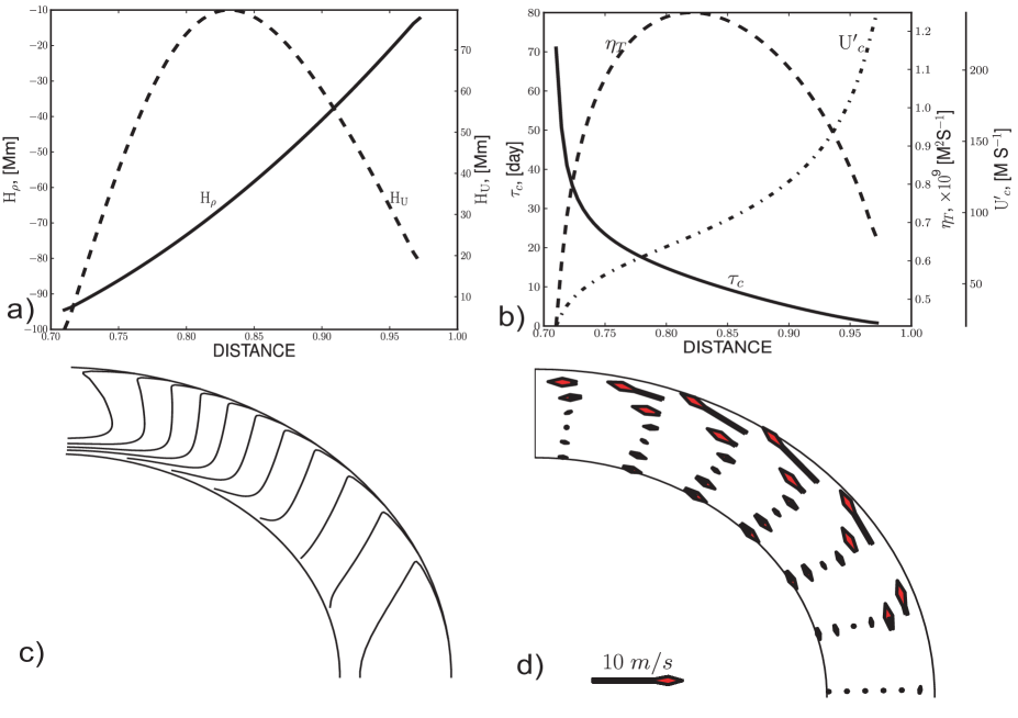
Figure 1: Internal parameters of the solar convection zone: a), the density scale $H_{\rho}=G^{-1}$ (solid line), and the turbulent velocity scale $H_{U}={\displaystyle{(\nabla\log\bar{u^{2}})^{-1}}}$ (dashed line), the distance is measured in units of the solar radius; b) the typical turnover convective time, $\tau_{c}$ (solid line), the coefficient of the turbulent diffusivity, $\eta_{T}$, (dashed line), the RMS of convective velocity $u^{\prime}$(dash-dot line); c) the contours of the constant angular velocity are plotted for the levels $(0.75-1.05)\Omega_{0}$; d) the geometry of meridional circulation, the length of arrows are proportional to the circulation speed.

4 The $\overline{u_{r}b_{r}}$ patterns by dynamo models

In the next section, we illustrate contributions of each term to the correlation of the radial components, $\overline{u_{r}b_{r}}$, given by Eq.(17) for two types of solar dynamo models: the mean-field dynamo distributed in the convection zone and the benchmark flux-transport dynamo. The distributed dynamo model is described in detail by Pipin & Seehafer (2009) and Seehafer & Pipin (2009), hereafter, PS09 and SP09, respectively. The benchmark model was constructed by Jouve et al. (2008). We consider the large-scale magnetic field produced by the models as an input parameter for estimation of $\overline{u_{r}b_{r}}$ in Eq.(17). The dynamo equations are given in Appendix B.

The distributed dynamo model includes the meridional circulation with the geometry of flow which is similar to that used by Bonanno et al. (2002). The maximum velocity of the meridional circulation is fixed to 10 $\mathrm{ms^{-1}}$. The turbulent generation effects include the $\alpha-$effect (Parker, 1955) and the ${\boldmath\mathbf{\Omega}}\times\mathbf{J}$ effect (Rädler, 1969). The internal parameters of the solar convection zone are given by Stix (2002). The integration domain is above the tachocline, from 0.71$R_{\odot}$ to 0.972$R_{\odot}$ in radius, and from the pole to the pole in latitude. We use the differential rotation profile given by Antia et al. (1998). The internal parameters of the model, including the turbulence parameters and parameters of stratification of solar convection zone, distribution of the angular velocity and the geometry of the meridional circulation are shown in Figure 1.

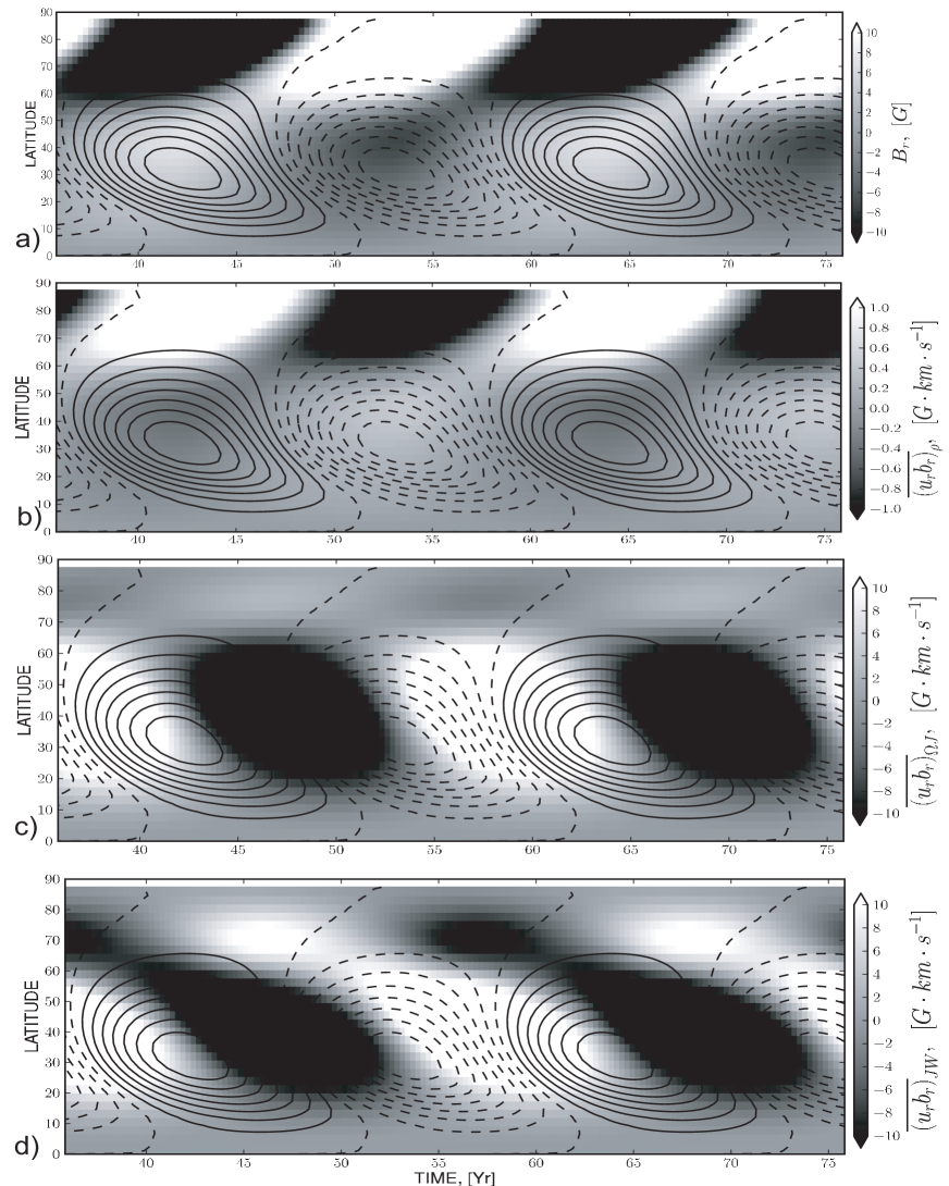
Figure 2: The time-latitude (“butterfly”) diagrams for the distributed dynamo model. Contours in each plot the toroidal magnetic field at the bottom of the convection zone. The color background shows: a) the large-scale radial magnetic field at the surface; b) the cross-helicity component $\left(\overline{u_{r}b_{r}}\right)_{\rho}$; c) $\left(\overline{u_{r}b_{r}}\right)_{\Omega J}$ ; d) $\left(\overline{u_{r}b_{r}}\right)_{JW}$, defined in Eq. (17,3.2).

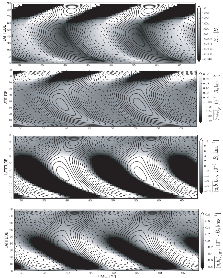
Figure 3: The same as in Fig.2 for the flux-transport dynamo model.

For comparison we examine the $\overline{u_{r}b_{r}}$ patterns of the benchmark flux-transport dynamo model. This type of dynamo models is one of those widely discussed in the literature (e.g., Bonanno et al., 2002; Dikpati et al., 2004). We keep the same formulation of the benchmark dynamo model as described by Jouve et al. (2008), although we use the same type of rotation law as in the previous subsection. The integration domain in this model is from $0.65R_{\odot}$ to $0.97R_{\odot}$. The calculation of the $\overline{u_{r}b_{r}}$ is carried out from $0.71R_{\odot}$ to $0.97R_{\odot}$. The magnetic field in this benchmark model is measured in the units of $B_{0}$. Therefore the calculated cross-helicity is scaled with the magnetic field strength $B_{0}$. The other parameters of the model are: the reference turbulent diffusivity, $5\cdot 10^{10}\mathrm{cm^{2}s^{-1}}$ ($C_{\eta}=0.005$), the magnetic Reynolds number, $\mathrm{Rm}=700$, the coefficient of the poloidal magnetic field source term, $C_{s}=30$ (in notations of Jouve et al., 2008).

We separate contributions to $\overline{u_{r}b_{r}}$ into three parts: $\left(\overline{u_{r}b_{r}}\right)_{\rho}$ , $\left(\overline{u_{r}b_{r}}\right)_{\Omega J}$ and $\left(\overline{u_{r}b_{r}}\right)_{JW}$, and associate the first term of Eq.(17) as a contribution of the stratification effects, while the second and third terms represent contributions of the large-scale electric current. In the calculations we assume the equipartition between the kinetic and magnetic energies of fluctuations, $\varepsilon=1$. Modeling the cross-helicity we found that if we take the surface values for the model quantities in Eq.(17) then we obtain that the stratification effects are dominant. This is true for the both types of dynamo models. However, if we integrate the cross-helicity from the surface down to deeper layers, say down to $0.9R_{\odot}$, then the contributions of the large-scale current becomes comparable to the stratification effects and even greater. The dynamo butterfly diagrams and the simulated patterns of the cross-helicity variations are shown in Figures 2 and 3. In the simulations, the antisymmetric modes of the toroidal magnetic field are dominant. Therefore we show the butterfly diagram only for the northern hemisphere. The butterfly diagram of the toroidal magnetic field is shown for the bottom of the convection zone (from where the magnetic field of active regions presumably erupts), while the radial magnetic field patterns are shown for the top of the integration domain. In the first model the toroidal magnetic field strength varies with the amplitude of $2.5$kG at the bottom of the convection zone. The radial magnetic field has the maximum of the magnitude variations at the poles, where it varies with an amplitude of $40$G at the surface. The cross-helicity varies with amplitude $\pm 10\ \mathrm{G\cdot km\cdot s^{-1}}$. In the second model, the magnetic field strength is measured in the units of $B_{0}$, which is assumed to be the maximum of the typical strength of the flux tubes accumulated just beneath the solar convection zone (Dikpati & Charbonneau, 1999). The cross-helicity in the flux-transport model is scaled with $B_{0}$ as well. In this model, $B_{0}$ should be about $10^{5}$G in order to obtain the cross-helicity values similar to the previous model. The main reason for such high $B_{0}$ value is, of course, the low magnetic diffusivity used in the model. As shown by Dikpati et al. (2004), the flux-transport models can be tuned for high magnetic diffusivity in the near surface layers. In both cases, one can see that the part of the cross-helicity, which results from the density and turbulence stratification effects ( panel (b) of the Figures 2 and 3), follows the evolution of the radial magnetic fields while the large-scale current produces a more complicated pattern of the cross-helicity of comparable magnitude, panels (c) and (d). Both models give somewhat similar predictions for the cross-helicity patterns. The most obvious difference is that the second model predicts a very strong amplitude of the cross-helicity near the poles. This effect results from the strong polar magnetic field which varies in the range of $\pm 0.3B_{0}$ while the toroidal magnetic field in this model varies in the range of $\pm 3B_{0}$. In Figure 3, in order to resolve the fine structure of the sunspot formation zone we restrict variations of $B_{r}$ within the limits of $\pm 0.01B_{0}$. Comparing with observations, the polar magnetic field seems to be too strong in the benchmark flux-transport model. Perhaps this model needs further tuning in a way similar to given by Dikpati et al. (2004). Looking at the contribution of the cross-helicity produced by the large-scale current we find that in the distributed dynamo model the surface cross-helicity pattern correlates with the variations of $\bar{J_{r}}$, and in the flux-transport model both components of the current are important. The large-scale distribution of electric currents can be deduced from synoptic magnetogram (Pevtsov & Latushko, 2000; Wang & Zhang, 2009). For the current theory it would be interesting to compare the spatial-temporal patterns of the cross-helicity and the large-scale current. These patterns will evolve in phase if the contribution of the electric current in Eq(3.2) dominates.

If we consider the observational problem of finding the $\overline{u_{r}b_{r}}$, we have to choose suitable spatial and temporal scales for averaging (in the spirit of Zhang et al., 2010), in order to distinguish between the processes of the “local” (noted in Mason et al., 2006; Matthaeus et al., 2008) and “global” alignments of velocity and magnetic fields. We can take as a working hypothesis that for larger scales most contribution to the observed cross-helicity comes from deeper layers of the solar convective zone. This assumption is consistent with our approximations but requires further investigations. In particular, our study neglects turbulent fluxes of the cross-helicity. This assumes that the spatial scale for averaging exceeds the typical scale of the turbulent velocity variations.

5 Discussion

In this paper using the mean-field magnetohydrodynamics framework we derive an equation for the cross-helicity evolution in the presence of the large-scale magnetic fields and flows. This equation (see Eq.(12)) can be used to construct the mean-field dynamo model based on the cross-helicity effects (see, Yoshizawa et al., 2000; Sur & Brandenburg, 2009). It is also can be used to estimate the cross-helicity distribution in subsurface layer of the Sun. The structure of the cross-helicity source terms in the evolution equation was studied on the base of the MHD equations governing turbulent fluctuations of velocity and magnetic fields in stratified media in the presence of the large-scale magnetic fields and shear flow. We calculated the contributions of various effects to the cross-helicity pseudo-scalar. For comparison with solar observations we calculated the correlation of the radial components of the turbulent velocity and magnetic field and estimated these contributions for two different types of the solar dynamo.

Our results show that the turbulent cross-helicity reflects internal properties of the dynamo processes and allow us to discriminate among different solar dynamo models. For analysis of the observational data involving the cross-helicity it is important to consider averaging over small and large scales. If cross-helicity data are averaged over a small portion of the solar surface and short time periods, the results may contain mainly the effect of the density stratification and the vertical component of the large-scale magnetic field as shown by Rüdiger et al. (2010). However, this type of averaging may meet some practical problems because of the difficulty to distinguish between the processes of the global and local alignment, of the turbulent velocity and magnetic fields. For instance a similar kind of alignment for velocity and vorticity is known as kinetic helicity (see Pelz et al., 1985). However, for different scales of convection motions near the surface level one may observe different signs of the kinetic helicity at different depths (Zhao, 2004).

If the cross-helicity data are averaged over large spatial and temporal scales, then other effects related to the solar dynamo may become important (see Eq.(12)). In particular, the cross-helicity patterns depend on the distribution of large-scale electric currents and velocity shear. In this case, the analysis becomes more complicated, and the large-scale transport of cross-helicity represented by $\overline{\mathcal{F}}^{C}$ (see Eq.(10)) has to be taken into account. Furthermore, the cross-helicity equations (3.2) and (17), may become invalid in the deeper layers of the Sun due to the strong Coriolis force effects ($\Omega^{\star}\gg 1$).

Our study is done in the anelastic approximation and does not take into account the density fluctuations effects. However, it is known (e.g., Kichatinov & Pipin, 1993) that in the turbulent coefficients the density fluctuations effects comes with factor $g\bar{u^{2}}/C_{s}^{2}\approx\bar{u^{2}}/|H_{\rho}|$, and may become important. Therefore, we anticipate further development of the present theory regarding the turbulent transport and compressibility effects. In this paper, we have shown that the spatially-temporal patterns of cross-helicity depend on details of the dynamo mechanism. This suggests to use the cross-helicity tracer as a diagnostic tool for solar dynamo models. The forthcoming analysis of space and ground based observations towards direct determination of the cross-helicity challenges the future theoretical studies.

Acknowledgments.

This work was funded by the National Natural Science Foundation of China (NSFC), National Basic Research Program of China under grant 2000078401 and 2006CB806301, and Chinese Academy of Sciences under grant KLCX2-YW-T04 and the CAS Visiting Professorships for Senior International Scientists, as well as joint Chinese-Russian collaborative project of NNSF of China and RFBR of Russia under grant 08-02-92211, and also RFBR grant 10-02-00148-a, 10-02-00960 and NASA LWS NNX09AJ85G grant.

Appendix A. Calculation of the cross-helicity in $\tau$-approximation in Fourier space

Our approach for calculation of the cross-helicity is presented in detail by Pipin (2008), hereafter, P08. The important steps in procedure were described earlier (see, e.g., Rogachevskii & Kleeorin, 2000; Rädler et al., 2003 and Brandenburg & Subramanian, 2005). The calculation is based on the equations governing the evolution of the fluctuating velocity and magnetic fields in a rotating coordinate system (see, also, Rogachevskii & Kleeorin, 2000; Rädler et al., 2003; Pipin, 2008):

$$\frac{\partial\mathbf{b}}{\partial t}\!\! = \!\!\!\!\nabla\!\times\!\left(\mathbf{u}\times\mathbf{\overline{B}}\!+\!\mathbf{\overline{U}}\times\mathbf{b}\right)\!+\!\eta\nabla^{2}\mathbf{b}\!+\!{\mathfrak{G}}\,,$$ (20)

$$\frac{\partial m_{i}}{\partial t} = -2\left(\mathbf{\Omega}\times\mathbf{m}\right)_{i}-\nabla_{i}\left(p^{\prime}-\frac{2}{3}\left(\mathbf{G\cdot m}\right)\nu+\frac{\left(\mathbf{b\cdot\overline{B}}\right)}{2\mu}\right)$$

$$+ \nu\Delta m_{i}+\nu\left(\mathbf{G\cdot\nabla}\right)m_{i}+f_{i}+\mathfrak{F}_{i}$$

$$+ \frac{1}{\mu_{0}}\nabla_{j}\left(\overline{B}_{j}b_{i}+\overline{B}_{i}b_{j}\right)-\nabla_{j}\left(\overline{U}_{j}m_{i}+\overline{U}_{i}m_{j}\right)\,.$$

They can be obtained from Eqs(3,4) by splitting velocity and magnetic fields into the mean and fluctuating part (see Eq.(1)). Here, $\mathfrak{G}$, and $\mathfrak{F}$ stand for unspecified nonlinear contributions of the fluctuating fields, ${\mathbf{m}}=\bar{\rho}{\mathbf{u}}$, $\mathbf{G}=\nabla\log\bar{\rho}$ is the density stratification scale of the media, $p^{\prime}$ the fluctuating pressure component, $\mathbf{\Omega}$ is the angular velocity responsible for the Coriolis force, $\mathbf{\overline{U}}$ is the mean flow velocity, weakly varying in space, and $\mathbf{f}$ is a random force driving the turbulence, $\eta$ and $\nu$ are the microscopic magnetic diffusivity and viscosity, respectively. The further calculation is done as follows. First, it is convenient to write equations (20) and (Appendix A. Calculation of the cross-helicity in $\tau$-approximation in Fourier space) in the Fourier space:

$$\left(\frac{\partial}{\partial t}+\eta z^{2}\!\!\right)\hat{b}_{j}(\mathbf{z})\!\! = \!\!\mathrm{i}z_{l}\!\!\int\!\!\left[\widehat{m}_{j}(\mathbf{z-q)}\hat{\left(\frac{\overline{B}_{l}}{\rho}\right)}(\mathbf{q})-\widehat{m}_{l}(\mathbf{z-q)}\hat{\left(\frac{\overline{B}_{j}}{\rho}\right)}(\mathbf{q})\right]\mathrm{{d}}\mathbf{q}$$

$$+ \mathrm{i}z_{l}\int\left[\widehat{b}_{l}(\mathbf{z-q)}\hat{\overline{V}}_{j}(\mathbf{q})-\widehat{b}_{j}(\mathbf{z-q)}\hat{\overline{V}}_{l}(\mathbf{q})\right]\mathrm{{d}}\mathbf{q}+\widehat{{\mathfrak{G}}}_{j}.$$

$$\left(\frac{\partial}{\partial t}+\nu z^{2}+\mathrm{i}\nu\left(\mathbf{Gz}\right)\right)\hat{m}_{i}(\mathbf{z}) = \hat{f}_{i}+\hat{\mathfrak{F}}_{i}-2\left(\mathbf{\Omega}\hat{\mathbf{z}}\right)\left(\hat{\mathbf{z}}\times\hat{\mathbf{m}}\right)_{i}$$

$$- \mathrm{i}\pi_{if}(\mathbf{z)}z_{l}\int\left[\widehat{m}_{l}(\mathbf{z-q)}\hat{\overline{V}}_{f}(\mathbf{q})+\widehat{m}_{f}(\mathbf{z-q)}\hat{\overline{V}}_{l}(\mathbf{q})\right]\mathrm{{d}}\mathbf{q}$$

$$+ \frac{\mathrm{i}}{\mu}\pi_{if}(\mathbf{z)}z_{l}\int\left[\widehat{b}_{l}(\mathbf{z-q)}\hat{\overline{B}}_{f}\left({\mathbf{q}}\right)+\widehat{b}_{f}(\mathbf{z-q)}\hat{\overline{B}}_{l}\left(q\right)\right]\mathrm{{d}}\mathbf{q},$$

where the turbulent pressure was excluded from (Appendix A. Calculation of the cross-helicity in $\tau$-approximation in Fourier space) by convolution with tensor $\pi_{ij}(\mathbf{z)}=\delta_{ij}-\hat{z}_{i}\hat{z}_{j}$, $\delta_{ij}$ is the Kronecker symbol and $\hat{\mathbf{z}}$ is a unit wave vector. The equations for the second-order moments that make contributions to the cross-helicity tensor can be found directly from (Appendix A. Calculation of the cross-helicity in $\tau$-approximation in Fourier space,Appendix A. Calculation of the cross-helicity in $\tau$-approximation in Fourier space). As the preliminary step we write the equations for the second-order products of the fluctuating fields, and make the ensemble averaging of them,

$$\frac{\partial}{\partial t}\left\langle\hat{m}_{i}\left(\mathbf{z}\right)\hat{b}_{j}\left(\mathbf{z}^{\prime}\right)\right\rangle = Th_{ij}^{\varkappa}(\mathbf{z},\mathbf{z^{\prime}})-\left(\eta z^{\prime 2}+\nu z^{2}+\mathrm{i}\nu\left(\mathbf{Gz}\right)\right)\left\langle\hat{m}_{i}\left(\mathbf{z}\right)\hat{b}_{j}\left(\mathbf{z}^{\prime}\right)\right\rangle$$

$$\mathrm{i}z^{\prime}_{l}\int\left[\left\langle\hat{m}_{i}\left(\mathbf{z}\right)\hat{m}_{j}(\mathbf{z^{\prime}-q)}\right\rangle\hat{\left(\frac{\overline{B}_{l}}{\rho}\right)}(\mathbf{q})-\right.$$

$$- \left.\left\langle\hat{m}_{i}\left(\mathbf{z}\right)\hat{m}_{l}(\mathbf{z^{\prime}-q)}\right\rangle\hat{\left(\frac{\overline{B}_{j}}{\rho}\right)}(\mathbf{q})\right]\mathrm{d}\mathbf{q}-2\left(\mathbf{\Omega}\hat{\mathbf{z}}\right)\varepsilon_{iln}\hat{z_{l}}\left\langle\hat{m_{n}}(\mathbf{z})\hat{b}_{j}(\mathbf{z^{\prime}})\right\rangle$$

$$+ \mathrm{i}z^{\prime}_{l}\int\left[\left\langle\hat{m}_{i}\left(\mathbf{z}\right)\widehat{b}_{l}(\mathbf{z^{\prime}-q)}\right\rangle\hat{\overline{V}}_{j}(\mathbf{q})-\left\langle\hat{m}_{i}\left(\mathbf{z}\right)\widehat{b}_{j}(\mathbf{z^{\prime}-q)}\right\rangle\hat{\overline{V}}_{l}(\mathbf{q})\right]\mathrm{{d}}\mathbf{q}$$

$$- \mathrm{i}\pi_{if}(\mathbf{z)}z_{l}\int\left[\left\langle\widehat{m}_{l}(\mathbf{z-q)}\hat{b}_{j}\left(\mathbf{z}^{\prime}\right)\right\rangle\hat{\overline{V}}_{f}(\mathbf{q})+\left\langle\widehat{m}_{f}(\mathbf{z-q)}\hat{b}_{j}\left(\mathbf{z}^{\prime}\right)\right\rangle\hat{\overline{V}}_{l}(\mathbf{q})\right]\mathrm{{d}}\mathbf{q}$$

$$+ \frac{\mathrm{i}}{\mu}z_{l}\pi_{if}(\mathbf{z)}\int\left[\left\langle\widehat{b}_{l}(\mathbf{z-q)}\hat{b}_{j}\left(\mathbf{z}^{\prime}\right)\right\rangle\overline{B}_{f}\left(\mathbf{q}\right)+\left\langle\widehat{b}_{f}(\mathbf{z-q)}\hat{b}_{j}\left(\mathbf{z}^{\prime}\right)\right\rangle\overline{B}_{l}\left(q\right)\right]\mathrm{d}\mathbf{q},$$

$$\frac{\partial}{\partial t}\left\langle\hat{m}_{i}\left(\mathbf{z}\right)\hat{m}_{j}\left(\mathbf{z}^{\prime}\right)\right\rangle = -2\left(\mathbf{\Omega}\hat{\mathbf{z}}\right)\varepsilon_{iln}\hat{z_{l}}\left\langle\hat{m_{n}}(\mathbf{z})\hat{m}_{j}(\mathbf{z^{\prime}})\right\rangle-2\left(\mathbf{\Omega}\hat{\mathbf{z}}^{\prime}\right)\varepsilon_{jln}\hat{z_{l}^{\prime}}\left\langle\hat{m_{i}}(\mathbf{z})\hat{m}_{n}(\mathbf{z^{\prime}})\right\rangle$$

$$- \mathrm{i}\pi_{if}(\mathbf{z)}z_{l}\int\left[\left\langle\widehat{m}_{l}(\mathbf{z-q)}\hat{m}_{j}\left(\mathbf{z}^{\prime}\right)\right\rangle\hat{\overline{V}}_{f}(\mathbf{q})+\left\langle\widehat{m}_{f}(\mathbf{z-q)}\hat{m}_{j}\left(\mathbf{z}^{\prime}\right)\right\rangle\hat{\overline{V}}_{l}(\mathbf{q})\right]\mathrm{{d}}\mathbf{q}$$

$$- \mathrm{i}\pi_{jf}(\mathbf{z^{\prime})}z^{\prime}_{l}\int\left[\left\langle\hat{m}_{i}\left(\mathbf{z}\right)\widehat{m}_{l}(\mathbf{z-q)}\right\rangle\hat{\overline{V}}_{f}(\mathbf{q})+\left\langle\hat{m}_{i}\left(\mathbf{z}\right)\widehat{m}_{f}(\mathbf{z-q)}\right\rangle\hat{\overline{V}}_{l}(\mathbf{q})\right]\mathrm{{d}}\mathbf{q}$$

$$+ \frac{\mathrm{i}}{\mu}\pi_{if}\left(\mathbf{z}\right)z_{l}\int\left[\left\langle\widehat{b}_{l}(\mathbf{z-q)}\hat{m}_{j}\left(\mathbf{z}^{\prime}\right)\right\rangle\hat{\overline{B}}_{f}\left({\mathbf{q}}\right)+\left\langle\widehat{b}_{f}(\mathbf{z-q)}\hat{m}_{j}\left(\mathbf{z}^{\prime}\right)\right\rangle\hat{\overline{B}}_{l}\left(q\right)\right]\mathrm{{d}}\mathbf{q}$$

$$+ \frac{\mathrm{i}}{\mu}\pi_{jf}(\mathbf{z^{\prime})}z^{\prime}_{l}\int\left[\left\langle\hat{m}_{i}\left(\mathbf{z}\right)\widehat{b}_{l}(\mathbf{z-q)}\right\rangle\hat{\overline{B}}_{f}\left({\mathbf{q}}\right)+\left\langle\hat{m}_{i}\left(\mathbf{z}\right)\widehat{b}_{f}(\mathbf{z-q)}\right\rangle\hat{\overline{B}}_{l}\left(q\right)\right]\mathrm{{d}}\mathbf{q}$$

$$+ Th_{ij}^{v}(\mathbf{z},\mathbf{z^{\prime}})-\nu\left(z^{\prime 2}+z^{2}+i\left(\mathbf{Gz}\right)+i\left(\mathbf{Gz^{\prime}}\right)\right)\left\langle\hat{m}_{i}\left(\mathbf{z}\right)\hat{m}_{j}\left(\mathbf{z}^{\prime}\right)\right\rangle,$$

$$\frac{\partial}{\partial t}\left\langle\hat{b}_{i}\left(\mathbf{z}\right)\hat{b}_{j}\left(\mathbf{z}^{\prime}\right)\right\rangle = Th_{ij}^{h}(\mathbf{z},\mathbf{z^{\prime}})-\left(\eta z^{\prime 2}+\eta z^{2}\right)\left\langle\hat{b}_{i}\left(\mathbf{z}\right)\hat{b}_{j}\left(\mathbf{z}^{\prime}\right)\right\rangle$$

$$+ \mathrm{i}z^{\prime}_{l}\int\left[\left\langle\hat{b}_{i}\left(\mathbf{z}\right)\hat{m}_{j}(\mathbf{z^{\prime}-q)}\right\rangle\hat{\left(\frac{\overline{B}_{l}}{\rho}\right)}(\mathbf{q})-\left\langle\hat{b}_{i}\left(\mathbf{z}\right)\hat{m}_{l}(\mathbf{z^{\prime}-q)}\right\rangle\hat{\left(\frac{\overline{B}_{j}}{\rho}\right)}(\mathbf{q})\right]\mathrm{d}\mathbf{q}$$

$$+ \mathrm{i}z_{l}\int\left[\left\langle\hat{m}_{i}(\mathbf{z-q)}\hat{b}_{j}\left(\mathbf{z}^{\prime}\right)\right\rangle\hat{\left(\frac{\overline{B}_{l}}{\rho}\right)}(\mathbf{q})-\left\langle\hat{m}_{l}(\mathbf{z-q)}\hat{b}_{j}\left(\mathbf{z}^{\prime}\right)\right\rangle\hat{\left(\frac{\overline{B}_{i}}{\rho}\right)}(\mathbf{q})\right]\mathrm{d}\mathbf{q}$$

$$+ \mathrm{i}z^{\prime}_{l}\int\left[\left\langle\hat{b}_{i}\left(\mathbf{z}\right)\widehat{b}_{l}(\mathbf{z^{\prime}-q)}\right\rangle\hat{\overline{V}}_{j}(\mathbf{q})-\left\langle\hat{b}_{i}\left(\mathbf{z}\right)\widehat{b}_{j}(\mathbf{z^{\prime}-q)}\right\rangle\hat{\overline{V}}_{l}(\mathbf{q})\right]\mathrm{{d}}\mathbf{q},$$

where, the terms $Th_{ij}^{(\varkappa,v,h)}$ involve the third-order moments of fluctuating fields and second-order moments of them with the forcing term. To proceed further we introduce the double Fourier transformation of an ensemble average of two fluctuating quantities, say $f$ and $g$, taken at identical times and at the different positions $\mathbf{x},\,\mathbf{x}^{\prime}$, is given by

$$\overline{f\left(\mathbf{x}\right)g\left(\mathbf{x}^{\prime}\right)}\!=\!\int\int\overline{\hat{f}\left(\mathbf{z}\right)\hat{g}\left(\mathbf{z}^{\prime}\right)}e^{\mathrm{i}\left(\mathbf{z}\cdot\mathbf{x}+\mathbf{z}^{\prime}\cdot\mathbf{x}^{\prime}\right)}\mathrm{d}^{3}\mathbf{z}\mathrm{d}^{3}\mathbf{z}^{\prime}.$$ (27)

In the spirit of the general formalism of the two-scale approximation (Roberts & Soward, 1975) we introduce “fast” and “slow” variables. They are defined by the relative $\mathbf{r}=\mathbf{x}-\mathbf{x}^{\prime}$ and mean $\mathbf{R}=\left(\mathbf{x}+\mathbf{x}^{\prime}\right)/2$, coordinates respectively. The fast and slow variables in the Fourier space correspond to two wave vectors: $\mathbf{k}=\left(\mathbf{z}-\mathbf{z}^{\prime}\right)/2$ and $\mathbf{K}=\mathbf{z}+\mathbf{z}^{\prime}$. Then, we define a correlation function of $\hat{\mathbf{f}}$ and $\hat{\mathbf{g}}$ obtained from Eq.(27) by integration with respect to $\mathbf{K}$,

$$\Phi\left(\hat{f},\hat{g},\mathbf{k},\mathbf{R}\right)=\int\overline{\hat{f}\left(\mathbf{k}+\frac{\mathbf{K}}{2}\right)\hat{g}\left(\frac{\mathbf{K}}{2}-\mathbf{k}\right)}\mathrm{e}^{\mathrm{i}\left(\mathbf{K}\cdot\mathbf{R}\right)}\mathrm{d}^{3}\mathbf{K}.$$ (28)

For further convenience we define the following second-order correlations of the momentum density, magnetic fluctuations, and cross-correlations of the momentum and magnetic fluctuations:

$$\hat{v}_{ij}\left(\mathbf{k},\mathbf{R}\right)\!\! \!=\! \!\!\Phi(\hat{m}_{i},\hat{m}_{j},\mathbf{k},\mathbf{R}),$$

$$\bar{\rho}^{2}\bar{\mathbf{u}^{2}}\left(\mathbf{R}\right)\! = \!\int\!\!\hat{v}_{ii}\left(\mathbf{k},\mathbf{R}\right)\mathrm{d}^{3}\mathbf{k},$$

$$\hat{h}_{ij}\left(\mathbf{k},\mathbf{R}\right)\!\! \!=\! \!\!\Phi(\hat{b}_{i},\hat{b}_{j},\mathbf{k},\mathbf{R}),$$

$$\bar{\mathbf{b}^{2}}\left(\mathbf{R}\right)\!\! = \!\!\int\!\!\hat{h}_{ii}\left(\mathbf{k},\mathbf{R}\right)\mathrm{d}^{3}\mathbf{k},$$ (29)

$$\hat{\varkappa}_{ij}\left(\mathbf{k},\mathbf{R}\right) = \Phi(\hat{m}_{i},\hat{b}_{j},\mathbf{k},\mathbf{R}),$$

We now return to equations (Appendix A. Calculation of the cross-helicity in $\tau$-approximation in Fourier space), (Appendix A. Calculation of the cross-helicity in $\tau$-approximation in Fourier space) and (Appendix A. Calculation of the cross-helicity in $\tau$-approximation in Fourier space). As the first step, we approximate the $Th_{ij}^{(\varkappa,v,h)}$-terms by the corresponding $\tau$ relaxation terms of the second-order contributions,

$$Th_{ij}^{(\varkappa)} \approx -\frac{\left\langle\hat{m}_{i}\left(\mathbf{z}\right)\hat{b}_{j}\left(\mathbf{z}^{\prime}\right)\right\rangle}{\tau_{c}},$$ (30)

$$Th_{ij}^{(v)} \approx -\frac{\left\langle\hat{m}_{i}\left(\mathbf{z}\right)\hat{m}_{j}\left(\mathbf{z}^{\prime}\right)\right\rangle-\left\langle\hat{m}_{i}\left(\mathbf{z}\right)\hat{m}_{j}\left(\mathbf{z}^{\prime}\right)\right\rangle^{\left(0\right)}}{\tau_{c}},$$ (31)

$$Th_{ij}^{(h)} \approx -\frac{\left\langle\hat{b}_{i}\left(\mathbf{z}\right)\hat{b}_{j}\left(\mathbf{z}^{\prime}\right)\right\rangle-\left\langle\hat{b}_{i}\left(\mathbf{z}\right)\hat{b}_{j}\left(\mathbf{z}^{\prime}\right)\right\rangle^{(0)}}{\tau_{c}},$$ (32)

where the superscript ⁽⁰⁾ denotes the moments of the background turbulence. Here, $\tau_{c}$is independent on $\mathbf{k}$ and it is independent on the mean fields as well. As the next step we make the Taylor expansion with respect to the “slow” variables and take the Fourier transformation, (28), about them. The details of this procedure can be found in (Brandenburg & Subramanian, 2005). Furthermore, we consider the high Reynolds number limit (relevant for the solar turbulence) and discard the microscopic diffusion terms. Then we arrive to the evolution equation for the cross-helicity tensor (see, P08):

$$\frac{\partial\hat{\varkappa}_{ij}}{\partial t} = -\mathrm{i}\left(\mathbf{\overline{B}k}\right)\left(\frac{\hat{v}_{ij}}{\bar{\rho}}-\frac{\hat{h}_{ij}}{\mu_{0}}\right)+\frac{\left(\overline{\mathbf{B}}\nabla\right)}{2}\left(\frac{\hat{v}_{ij}}{\bar{\rho}}+\frac{\hat{h}_{ij}}{\mu_{0}}\right)$$

$$+ \frac{\left(\overline{\mathbf{B}}\mathbf{k}\right)}{2\bar{\rho}}G_{s}\frac{\partial\hat{v}_{ij}}{\partial k_{s}}-\frac{\left(\mathbf{G\overline{B}}\right)}{2\bar{\rho}}\hat{v}_{ij}-\frac{1}{\mu_{0}}\hat{k}_{i}\hat{k}_{f}\overline{B}_{f,l}\hat{h}_{lj}$$

$$+ \frac{1}{\bar{\rho}}G_{l}\hat{v}_{il}B_{j}+\frac{\hat{h}_{lj}\overline{B}_{i,l}}{\mu_{0}}-\frac{\hat{v}_{il}\overline{B}_{j,l}}{\bar{\rho}}-\frac{\hat{\varkappa}_{ij}}{\tau_{c}}+\overline{U}_{j,l}\hat{\varkappa}_{il}$$

$$- \frac{k_{l}\overline{B}_{l,f}}{2}\frac{\partial}{\partial k_{f}}\left[\frac{\hat{v}_{ij}}{\bar{\rho}}+\frac{\hat{h}_{ij}}{\mu_{0}}\right]-\overline{U}_{i,l}\hat{\varkappa}_{lj}+\left[\hat{k}_{i}\hat{k}_{f}\right.$$

$$- \left.-\frac{\mathrm{i}}{2k}\left(2\hat{k}_{i}\hat{k}_{f}\left(\mathbf{\hat{k}}\cdot\mathbf{\nabla}\right)-\hat{k}_{i}\nabla_{f}-\hat{k}_{f}\nabla_{i}\right)\right]\hat{\varkappa}_{lj}\overline{U}_{f,l}$$

$$- 2\left(\Omega\hat{k}\right)\hat{k}_{p}\varepsilon_{ipl}\hat{\varkappa}_{lj}-2\frac{\mathrm{i}}{k}\left(\Omega\hat{k}\right)\hat{k}_{p}\varepsilon_{ipl}\left(\hat{k}\nabla\right)\hat{\varkappa}_{lj}$$

$$+ \frac{\mathrm{i}}{k}\varepsilon_{ipl}\left(\left(\Omega\hat{k}\right)\nabla_{p}\hat{\varkappa}_{lj}+\hat{k}_{p}\left(\Omega\nabla\right)\hat{\varkappa}_{lj}\right)+k_{l}\overline{U}_{f,l}\frac{\partial\hat{\varkappa}_{ij}}{\partial k_{f}},$$

where $\hat{\mathbf{k}}$ is a unit wave vector, $\overline{U}_{f,l}\equiv\nabla_{l}\overline{U}_{f}$ and $\overline{B}_{f,l}\equiv\nabla_{l}\overline{B}_{f}$. The expressions for the Fourier image of cross-helicity pseudo-scalar can be obtained from Eq.(Appendix A. Calculation of the cross-helicity in $\tau$-approximation in Fourier space) if we assume quasi-stationarity (discarding the time-derivative terms). Then we solve the obtained equation in the linear approximation with respect to the large-scale fields and the Coriolis force and obtain the cross-helicity tensor $\hat{\varkappa}_{ij}$. After this we calculate the cross-correlations:

$$\overline{\mathbf{u}\cdot\mathbf{b}} = \frac{1}{\overline{\rho}}\int\!\!\hat{\varkappa}_{ii}\left(\mathbf{k},\mathbf{R}\right)\mathrm{d}^{3}\mathbf{k},$$ (34)

$$\overline{u_{r}b_{r}} = \frac{1}{\overline{\rho}}\int\!\!e_{i}^{(r)}e_{j}^{(r)}\hat{\varkappa}_{ij}\left(\mathbf{k},\mathbf{R}\right)\mathrm{d}^{3}\mathbf{k},$$ (35)

where $e_{i}^{(r)}$ is the unit vector in radial direction. For the final results we have to define the spectra of the background turbulence. We consider the case of stationary and quasi-isotropic background turbulence(Kichatinov, 1987),

$$\hat{v}_{ij} = \left\{\pi_{ij}\left(\mathbf{k}\right)+\frac{\mathrm{i}}{2k^{2}}\left(k_{i}\nabla_{j}-k_{j}\nabla_{i}\right)\right\}\frac{\bar{\rho}^{2}E\left(k,\mathbf{R}\right)}{8\pi k^{2}},$$ (36)

where $\pi_{ij}(\mathbf{k)}=\delta_{ij}-\hat{k}_{i}\hat{k}_{j}$, $\delta_{ij}$ is the Kronecker symbol, the spectral function $E(k,\mathbf{R})$ defines the intensity of the velocity fluctuations:

$$\overline{\mathbf{u}^{2}} = \int\frac{E\left(k,\mathbf{R}\right)}{4\pi k^{2}}\mathrm{d}^{3}\mathbf{k}.$$ (37)

Similarly for the magnetic fluctuations of the turbulence, by the spectral function $\mathcal{B}(k,\mathbf{R})$ :

$$\overline{\mathbf{b}^{2}} = \int\frac{\mathcal{B}\left(k,\mathbf{R}\right)}{4\pi k^{2}}\mathrm{d}^{3}\mathbf{k}.$$ (38)

The anisotropy in Eq.(36) is induced by inhomogeneity of the turbulence. However, the scale of inhomogeneity is assumed to be small compared to the typical scale of turbulent flows. Therefore, the turbulent anisotropy is small and the given model of the background turbulence is called as quasi-isotropic (Kichatinov, 1987). We omit the further cumbersome derivations, which are explained in detail in P08.

Appendix B. Dynamo model equations

The evolution of the axisymmetric magnetic field ($B$ being the azimuthal component of the magnetic field, $A$ is proportional to the azimuthal component of the vector potential) is governed by the following equations:

$$\frac{\partial A}{\partial t}\!\! \!\!=\!\! \!\!r\sin\theta\mathcal{E}_{\phi}+\frac{U_{\theta}\sin\theta}{r}\frac{\partial A}{\partial\mu}-U_{r}\frac{\partial A}{\partial r}$$ (39)

$$r\sin\theta\mathcal{E}_{\phi}\!\! \!\!=\!\! \!\!\phi_{6}^{(a)}C_{\alpha}\eta_{T}Gr\mu\sin\theta Bf_{12}^{(a)}$$

$$+ \psi_{\eta}\eta_{T}\left\{f_{2}^{(d)}+2f_{1}^{(a)}\right\}\frac{\partial^{2}A}{\partial r^{2}}$$

$$+ \psi_{\eta}\eta_{T}\left\{f_{2}^{(d)}+2f_{1}^{(a)}\right\}\frac{\left(1-\mu^{2}\right)}{r^{2}}\frac{\partial^{2}A}{\partial\mu^{2}}$$

$$+ \psi_{\delta}C_{\delta}\eta_{T}f_{4}^{(d)}\sin\theta\left(r\mu\frac{\partial B}{\partial r}+\left(1-\mu^{2}\right)\frac{\partial B}{\partial\mu}\right)$$

$$\frac{\partial B}{\partial t} = -\sin\theta\left(\frac{\partial\Omega}{\partial r}\frac{\partial A}{\partial\mu}-\frac{\partial\Omega}{\partial\mu}\frac{\partial A}{\partial r}\right)-\frac{\partial\left(rU_{r}B\right)}{\partial r}$$

$$+ \frac{\sin\theta}{r}\frac{\partial U_{\theta}B}{\partial\mu}+\frac{1}{r}\frac{\partial r\mathcal{E}_{\theta}}{\partial r}+\frac{\sin\theta}{r}\frac{\partial\mathcal{E}_{r}}{\partial\mu}$$

$$\frac{\sin\theta}{r}\frac{\partial\mathcal{E}_{r}}{\partial\mu} = \frac{\sin\theta}{r^{2}}\frac{\partial}{\partial\mu}\left(\eta_{T}\psi_{\eta}\left(f_{2}^{(d)}\right.\right.$$

$$+ \left.\left.2f_{1}^{(a)}\left(1-\mu^{2}\right)\right)\right)\frac{\partial\sin\theta B}{\partial\mu}$$

$$+ \frac{2f_{1}^{(a)}\sin\theta}{r^{2}}\frac{\partial}{\partial r}\psi_{\eta}\frac{\partial}{\partial\mu}\left(\mu\sin\theta B\right)+$$

$$+ \frac{f_{1}^{(a)}\sin\theta}{r}G\frac{\partial}{\partial\mu}\left(\psi_{\eta}\mu\sin\theta B\right)$$

$$\frac{1}{r}\frac{\partial r\mathcal{E}_{\theta}}{\partial r} = \frac{1}{r}\frac{\partial}{\partial r}\left(\eta_{T}\psi_{\eta}\left(f_{2}^{(d)}+2f_{1}^{(a)}\mu^{2}\right)\right)\frac{\partial rB}{\partial r}+$$

$$+ \frac{2\mu\sin\theta}{r}\frac{\partial}{\partial r}\eta_{T}f_{1}^{(a)}\psi_{\eta}\frac{\partial}{\partial\mu}\left(\sin\theta B\right)$$

$$- \frac{1}{r}\frac{\partial}{\partial r}r\psi_{\eta}\left(Gf_{3}^{(a)}+G(2\mu^{2}-1)f_{1}^{(a)}\right)B$$

where $\mu=\cos\theta$, $\theta$ is co-latitude. We use the same notations as in P08. Functions $f_{1,2}^{(a,d)}$ depend on the Coriolis number $\Omega^{*}=2\tau_{c}\Omega_{0}$, $\tau_{c}$ is a typical correlation time of the turbulent convection; functions $\phi_{6}^{(a)}$ and $\psi_{\eta,\delta}$ describe magnetic quenching and depend on $\beta=B/\sqrt{\mu_{0}\bar{\rho}\bar{u^{2}}}$, parameters $C_{\alpha},\,C_{\delta}$ control the contributions of the $\alpha$ and $\Omega\times J$ effects. In notations of P08, $\psi_{\eta}=\phi_{3}+\phi_{2}-2\phi_{1}$ and $\psi_{\delta}=\phi_{7}^{(w)}+\phi_{2}^{(w)}$. We introduce parameter $C_{\eta}$ to control the turbulent diffusion coefficient, $\eta_{T}=C_{\eta}\tau_{c}\bar{\mathbf{u}^{2}}/3$. Following to the linear analysis of PS09 and SP09 we choose $C_{\delta}=0.02,C_{\alpha}=C_{\delta}/2,C_{\eta}=0.1$. The dynamo equations with these input parameters give a solar-type dynamo solution.

References

- Antia et al. (1998) Antia, H. M., Basu, S., & Chitre, S. M. 1998, MNRAS, 298, 543
- Blackman & Brandenburg (2002) Blackman, E. G., & Brandenburg, A. 2002, Astrophys. J., 579, 379
- Blackman & Field (2002) Blackman, E. G., & Field, G. B. 2002, Physical Review Letters, 89, 265007
- Boldyrev et al. (2009) Boldyrev, S., Mason, J., & Cattaneo, F. 2009, ApJ, 699, L39
- Bonanno et al. (2002) Bonanno, A., Elstner, D., Rüdiger, G., & Belvedere, G. 2002, A&A, 390, 673
- Brandenburg & Subramanian (2005) Brandenburg, A., & Subramanian, K. 2005, Phys. Rep., 417, 1
- Dikpati & Charbonneau (1999) Dikpati, M., & Charbonneau, P. 1999, ApJ, 518, 508
- Dikpati et al. (2004) Dikpati, M., de Toma, G., Gilman, P. A., Arge, C. N., & White, O. R. 2004, ApJ, 601, 1136
- Field & Blackman (2002) Field, G. B., & Blackman, E. G. 2002, ApJ, 572, 685
- Gough (1969) Gough, D. O. 1969, Journal of Atmospheric Sciences, 26, 448
- Jouve et al. (2008) Jouve, L., et al. 2008, A&A, 483, 949
- Kichatinov (1987) Kichatinov, L. L. 1987, Geophysical and Astrophysical Fluid Dynamics, 38, 273
- Kichatinov & Pipin (1993) Kichatinov, L. L., & Pipin, V. V. 1993, A&A, 274, 647
- Kitchatinov & Ruediger (1995) Kitchatinov, L. L., & Ruediger, G. 1995, A&A, 299, 446
- Kleeorin et al. (2003) Kleeorin, N., Kuzanyan, K., Moss, D., Rogachevskii, I., Sokoloff, D., & Zhang, H. 2003, A&A, 409, 1097
- Kleeorin et al. (1996) Kleeorin, N., Mond, M., & Rogachevskii, I. 1996, A&A, 307, 293
- Krause & Rädler (1980) Krause, F., & Rädler, K.-H. 1980, Mean-Field Magnetohydrodynamics and Dynamo Theory (Berlin: Akademie-Verlag)
- Kuzanyan et al. (2007) Kuzanyan, K. M.; Pipin, V. V. & Zhang, H. 2007, Advances in Space Research, 2007, 39, 1694
- Mason et al. (2006) Mason, J., Cattaneo, F., & Boldyrev, S. 2006, Physical Review Letters, 97, 255002
- Matthaeus et al. (2008) Matthaeus, W. H., Pouquet, A., Mininni, P. D., Dmitruk, P., & Breech, B. 2008, Physical Review Letters, 100, 085003
- Moffat (1969) Moffat, H. 1969, J . Fluid Mech., 35, 117
- Orszag (1970) Orszag, S. A. 1970, Journal of Fluid Mechanics, 41, 363
- Pelz et al. (1985) Pelz, R. B., Yakhot, V., Orszag, S. A., Shtilman, L., & Levich, E. 1985, Physical Review Letters, 54, 2505
- Pevtsov & Latushko (2000) Pevtsov, A. A., & Latushko, S. M. 2000, ApJ, 528, 999
- Pipin (2008) Pipin, V. V. 2008, Geophysical and Astrophysical Fluid Dynamics, 102, 21
- Pipin & Seehafer (2009) Pipin, V. V., & Seehafer, N. 2009, A&A, 493, 819
- Rädler et al. (2003) Rädler, K., Kleeorin, N., & Rogachevskii, I. 2003, Geophysical and Astrophysical Fluid Dynamics, 97, 249
- Rädler (1969) Rädler, K.-H. 1969, Monats. Dt. Akad. Wiss., 11, 194
- Rädler & Rheinhardt (2007) Rädler, K.-H., & Rheinhardt, M. 2007, Geophysical and Astrophysical Fluid Dynamics, 101, 117
- Raedler (1980) Raedler, K.-H. 1980, Astronomische Nachrichten, 301, 101
- Roberts & Soward (1975) Roberts, P., & Soward, A. 1975, Astron. Nachr., 296, 49
- Rogachevskii & Kleeorin (2000) Rogachevskii, I., & Kleeorin, N. 2000, Phys. Rev. E, 61, 5202
- Rüdiger et al. (2010) Rüdiger, G., Kitchatinov, L. L., & Brandenburg, A. 2010, Sol. Phys., 241
- Scherrer et al. (1995) Scherrer, P. H., et al. 1995, Sol. Phys., 162, 129
- Seehafer & Pipin (2009) Seehafer, N., & Pipin, V. V. 2009, A&A, 508, 9
- Stix (2002) Stix, M. 2002, The Sun. An Introduction (Springer)
- Sur & Brandenburg (2009) Sur, S., & Brandenburg, A. 2009, MNRAS, 399, 273
- Vainshtein & Kitchatinov (1983) Vainshtein, S. I., & Kitchatinov, L. L. 1983, Geophys. Astrophys. Fluid Dynam., 24, 273
- Wang & Zhang (2009) Wang, C., & Zhang, M. 2009, Science in China G: Physics and Astronomy, 52, 1713
- Woltjer (1958) Woltjer, L. 1958, Proc. Nat. Acad. Sci., 44, 833
- Yokoi (1999) Yokoi, N. 1999, Physics of Fluids, 11, 2307
- Yoshizawa (1990) Yoshizawa, A. 1990, Physics of Fluids B, 2, 1589
- Yoshizawa et al. (2000) Yoshizawa, A., Kato, H., & Yokoi, N. 2000, ApJ, 537, 1039
- Zhang et al. (2010) Zhang, H., Sakurai, T., Pevtsov, A., Gao, Y., Xu, H., Sokoloff, D. D., & Kuzanyan, K. 2010, MNRAS, 402, L30
- Zhao (2004) Zhao, J. 2004, PhD thesis, Stanford University
- Zhao et al. (2011) Zhao, M. Y., Wang, X. F., & Zhang, H. Q. 2011, Sol. Phys., 39