C

We study the distance between symmetry-violating quantum field theories and the surface of symmetric theories. We use this notion to quantify how precise Lorentz symmetry is today, according to experimental data. The metric in parameter space is defined à la Zamolodchikov, from the two-point function of the Lagrangian perturbation. The distance is obtained minimizing the length of paths connecting the Lorentz-violating theory to the Lorentz surface. This definition depends on the Lagrangian used to formulate the theory, including total derivatives and the choice of coordinate frame. We eliminate such dependencies minimizing with respect to them. We derive a number of general formulas and evaluate the distance in the CPT-invariant, QED subsectors of the Standard Model Extension (SME) and the renormalizable high-energy-Lorentz-violating Standard Model. We study the properties of the distance and address a number of applications.

1 Introduction

Theories that explicitly violate Lorentz symmetry contain a large number of independent parameters. For various purposes, it can be useful to collect them into a single quantity that measures the “amount of violation”. In this paper we propose to achieve this goal computing the distance between the Lorentz-violating theory and the Lorentz-symmetric surface. More generally, we study the distance between symmetry-violating theories and the symmetric surface. We investigate the properties of the distance and calculate it in quantum electrodynamics, using the known experimental bounds on the parameters of the Lorentz violation [1].

When a symmetry is broken spontaneously, there typically exists one parameter $\mu$, such as the vacuum expectation value of a scalar field, that quantifies the amount of violation. At $\mu=0$ the symmetry is restored, while at $\mu\neq 0$ $\mu$ can be viewed as a measure of the violation. When a symmetry is violated explicitly, instead, the parameters of the violation are typically numerous. The distance between a symmetry-violating theory and the surface of symmetric theories is a single quantity that collects all parameters of the violation, and vanishes if and only if all of them vanish. When it is infinitesimal, it is a relatively simple positive-definite quadratic form. It can be useful for several purposes. First, it assigns a relative weight to each parameter of the violation. Some parameters may be more or less significant than others, in some limits or particular situations. This kind of knowledge may be useful to guide the experimental search. The notion of distance can also address the search for a unifying principle behind the violation, or a more fundamental completion of the theory. Finally, it can be useful also in effective field theory, because at low-energies a spontaneously broken symmetry may look indistinguishable from an explicitly broken symmetry.

We assume that a theory $\tau_{\mathcal{L}}$ is defined by a Lagrangian $\mathcal{L}$ and a quantization procedure, such as the functional integral. We start from the metric in parameter space, defined à la Zamolodchikov [2], from the two-point function of the infinitesimal Lagrangian perturbation. The metric defines the infinitesimal distance $\mathrm{d}\ell$ between two theories $\tau_{\mathcal{L}}$ in the usual way. Integrating $\mathrm{d}\ell$ along a path $\gamma$ gives the length of the path. The (finite) distance between two theories $\tau_{\mathcal{L}}$ is then the length of the shortest path connecting them. This definition is renormalization-group (RG) invariant and satisfies the axioms of a distance, but has some unusual features. For example, it strictly depends on the Lagrangian used to formulate the theory. Total derivatives and coordinate reparametrizations, among the other things, do affect the distance. A way to eliminate such dependencies is to suitably minimize with respect to equivalent Lagrangian formulations of the same theory.

The distance between a theory $\tau_{\mathcal{L}}$ and a surface $S$ of theories is the length of the shortest path connecting $\tau_{\mathcal{L}}$ to $S$. For theories infinitesimally close to $S$ it is sufficient to calculate the normal vector, for which we give a simple formula in terms of a “reduced metric” that incorporates the effects of the minimization.

Variations of parameters that do not move away from the symmetric surface will be called tangent displacements. Minimizing with respect to tangent displacements is necessary to find the closest point on the surface. When we consider variations of parameters introduced by reparametrizations of fields and coordinates, we speak of reparametrization-displacements. Minimizing with respect to reparametrization-displacements is a way to eliminate the ambiguities associated with the formulation of the theory. Alternatively, the ambiguities can be removed with conventional prescriptions. In some cases Lorentz-violating theories remove some of these ambiguities automatically, because they define a preferred reference frame.

We evaluate the distance in Lorentz-violating quantum electrodynamics. At low-energies, we consider the CPT-invariant sector of the Colladay-Kostelecky minimal Standard Model extension of [3], and use the data tables of ref. [1]. The minimizations with respect to tangent- and reparametrization-displacements give constraints that coincide with the conventions used in the literature.

Later we extend the calculation to the QED subsector of the Lorentz-violating Standard Model of ref.s [4, 5]. It includes higher-dimensional operators, but it is still renormalizable by weighted power counting [6]. In this case we use the bounds of ref. [7].

We also derive formulas for the most general CPT-invariant marginal Lorentz-violating deformations of free relativistic fields and study the conditions obtained minimizing with respect to tangent- and reparametrization-displacements.

Quantum electrodynamics is weakly coupled at all energies we are interested in, and most experimental bounds on the parameters of the Lorentz violation are very small. For this reason, one-loop results and the free-field limit are sufficient to calculate the distance to a first approximation. In the marginal sector, the relative weights assigned by the distance to Lorentz-violating parameters are simple numerical factors of order 1. Indeed, no very large or small numbers can be generated by one-loop diagrams involving marginal operators. This means that all marginal parameters are on an equal footing.

On the other hand, when higher-derivative operators are included, the relative weights can be larger numbers, and may lower the scale at which the effects of the Lorentz violation become important. The distance can be useful as a guiding quantity to identify which parameters at which energies are more significant to search for signs of Lorentz violation.

As mentioned earlier, the distance may depend on total derivatives added to the Lagrangian. In general, every dependence on unwanted parameters can be eliminated minimizing with respect to them. Then, however, formulas become considerably involved. Sometimes it may be convenient to fix suitable prescriptions instead of minimizing. We study several options, and show that the qualitative features of the distance are unaffected by these choices.

The paper is organized as follows. In section 2 we define the metric and the distance in parameter space. In section 3 we study the distance between a Lorentz-violating theory and the Lorentz surface, and derive some useful formulas, in particular when the distance is infinitesimal. In section 4 we study simple examples, such as infinitesimal and finite distances among massive and massless fields, and the case of spontaneously broken gauge symmetries. In section 5 we derive formulas for the most general marginal CPT-invariant Lorentz-violating deformations of free massless relativistic fields. In section 6 we evaluate the distance in Lorentz-violating quantum electrodynamics. We first focus on the low-energy limit and then include higher-derivative operators, in particular those predicted by the Lorentz-violating Standard Model of ref.s [4, 5]. In section 7 we study the dependence of the distance on total derivatives and coordinate reparametrizations. In the appendix we show that the distance is RG invariant.

We need to use both Minkowskian and Euclidean notations. All parameters used in our formulas are Minkowskian, which is convenient to emphasize the positive-definiteness of the distance, and make contact with existing parametrizations. The Euclidean notation is convenient to define and calculate the distance.

2 Metric and distance in parameter space

In this section we define the metric in parameter space, the length of a path, and the distance between theories and from a theory to a surface of theories.

We assume that a quantum field theory $\tau$ is described by a Lagrangian $\mathcal{L}$ and a quantization procedure. For definiteness, we may choose the functional-integral approach and the dimensional-regularization technique. A Lagrangian uniquely defines a theory, but the same theory can be described by different Lagrangians. We call $\mathcal{L}$-theory the theory $\tau$ as it is defined by the Lagrangian $\mathcal{L}$, and denote it with $\tau_{\mathcal{L}}$. We must first define the distance between two $\mathcal{L}$-theories, then the distance between two theories.

Given an $\mathcal{L}$-theory with Lagrangian $\mathcal{L}(\lambda)$ and couplings $\lambda^{I}$, consider a small perturbation

$$\mathcal{L}+\mathrm{d}\mathcal{L}=\mathcal{L}+\sum_{I}\mathrm{d}\lambda^{I}\mathcal{O}_{I}=\mathcal{L}(\lambda+\mathrm{d}\lambda),$$

where the $\mathcal{O}_{I}$s are local operators. The infinitesimal squared distance between $\tau_{\mathcal{L}}$ and $\tau_{\mathcal{L}+\mathrm{d}\mathcal{L}}$ at energy $E=1/\hat{x}$ is defined as

$$\mathrm{d}\ell^{2} = 2\pi^{4}\hat{x}^{8}\langle\mathrm{d}\mathcal{L}\left(\frac{x}{2}\right)\hskip 0.72229pt\hskip 0.72229pt\mathrm{d}\mathcal{L}^{\theta}\left(\frac{x^{\theta}}{2}\right)\rangle=2\pi^{4}\hat{x}^{8}\langle\mathrm{d}\mathcal{L}(\hat{x}_{v})\hskip 0.72229pt\hskip 0.72229pt\mathrm{d}\mathcal{L}^{\theta}(0)\rangle$$ (2.1)

$$= 2\pi^{4}\hat{x}^{8}\sum_{IJ}\mathrm{d}\lambda^{I}\langle\mathcal{O}_{I}(\hat{x}_{v})\hskip 0.72229pt\hskip 0.72229pt\mathcal{O}_{J}^{\theta}(0)\rangle\mathrm{d}\lambda^{J*}\equiv\sum_{IJ}\mathrm{d}\lambda^{I}g_{IJ}(\hat{x},\lambda)\mathrm{d}\lambda^{J\hskip 0.72229pt*},$$

where $\langle\cdots\rangle$ is the expectation value on the vacuum state of the unperturbed theory $\mathcal{L}$ in Euclidean space, $x=(\hat{x},\bar{x})$, $\hat{x}>0$, and $\hat{x}_{v}$ denotes the four-vector $(\hat{x},\mathbf{0})$. Hats denote time components and bars denote space components. In both Minkowski and Euclidean spaces time components will also be denoted with the index 0. Finally, $\theta$ denotes the operation of time reflection. On coordinates $x$ it acts as $x^{\theta}=(-\hat{x},\bar{x})$. On operators in Euclidean space it acts antilinearly and generates a factor $-1$ for every time index:

$$\mathcal{O}_{\mu\nu\cdots}^{\theta}=\mathcal{O}_{\mu\nu\cdots}^{\dagger}(-1)^{\delta_{\mu 0}}(-1)^{\delta_{\nu 0}}\cdots.$$

Writing (2.1) we have used translational invariance, which we assume here. We also assume that the $\mathcal{L}$-theory $\tau_{\mathcal{L}}$ is reflection positive. Instead, Lorentz invariance is not assumed. The normalization factor appearing in (2.1) will be explained later.

The infinitesimal squared distance $\mathrm{d}\ell^{2}$ defines the metric $g_{IJ}$ in parameter space:

$$g_{IJ}(\hat{x},\lambda)=2\pi^{4}\hat{x}^{8}\langle\mathcal{O}_{I}(\hat{x}_{v})\hskip 0.72229pt\mathcal{O}_{J}^{\theta}(0)\rangle,$$ (2.2)

which is a Hermitian matrix. Apart from the normalization factor, this formula agrees with Zamolodchikov’s definition [2]. We often work in a real basis, namely a basis where the parameters $\mathrm{d}\lambda^{I}$ are real, the operators $\mathcal{O}_{I}$ are Hermitian and the metric is symmetric.

If $-d_{I}$ denotes the canonical dimension of the parameter $\mathrm{d}\lambda^{I}$ in units of mass, we can write

$$\langle\mathcal{O}_{I}(\hat{x}_{v})\hskip 0.72229pt\mathcal{O}_{J}^{\theta}(0)\rangle=\frac{1}{2\pi^{4}}\frac{G_{IJ}(t,\hat{\lambda})}{\hat{x}^{8+d_{I}+d_{J}}},$$ (2.3)

where $t=-\ln(\hat{x}\mu)$, $\mu$ is the renormalization scale and $\hat{\lambda}^{I}=\hat{x}^{-d_{I}}\lambda$. Hence,

$$g_{IJ}=\hat{x}^{-d_{I}-d_{J}}G_{IJ}(t,\hat{\lambda})$$ (2.4)

and the infinitesimal distance can be expressed as

$$\mathrm{d}\ell=\sqrt{\mathrm{d}\hat{\lambda}^{I}\hskip 0.72229ptG_{IJ}(t,\hat{\lambda})\hskip 0.72229pt\mathrm{d}\hat{\lambda}^{*J}},$$ (2.5)

where $\mathrm{d}\hat{\lambda}^{I}=\hat{x}^{-d_{I}}\mathrm{d}\lambda^{I}$.

The $\hat{x}$ -dependence of the metric can be regarded as a dependence on the energy. Its meaning will be illustrated with explicit examples. In the appendix we prove that the distance $\mathrm{d}\ell$ is renormalization-group invariant. In particular, $\mathrm{d}\ell$ can be written in the manifestly RG-invariant form

$$\mathrm{d}\ell=\sqrt{\mathrm{d}\hat{\lambda}^{I}(t)\hskip 0.72229ptG_{IJ}(0,\hat{\lambda}(t))\hskip 0.72229pt\mathrm{d}\hat{\lambda}^{*J}(t)},$$

where $\hat{\lambda}^{I}(t)=\hat{x}^{-d_{I}}\lambda^{I}(t)$, and $\lambda^{I}(t)$ denote the running coupling constants.

By reflection positivity, $\mathrm{d}\ell$ is non-negative. Terms proportional to the field equations do not contribute to the distance, because they give contact terms in the two-point function $\langle\mathrm{d}\mathcal{L}(\hat{x}_{v})~{}\mathrm{d}\mathcal{L}(0)\rangle$, which are negligible because $\hat{x}_{v}\neq 0$.

Now we define the finite distance between two $\mathcal{L}$-theories $\tau_{\mathcal{L}_{1}}$ and $\tau_{\mathcal{L}_{2}}$ at some energy scale $E$. Let $\gamma_{12}$ denote a path in parameter space connecting $\mathcal{L}_{1}$ to $\mathcal{L}_{2}$, namely a curve

$$\gamma_{12}:\qquad\rho\in[0,1]\rightarrow\lambda^{I}(\rho),$$

where the values of the couplings are referred to the energy $E$ and $\lambda^{I}(0)$ and $\lambda^{I}(1)$ are such that $\mathcal{L}(\lambda(0))=\mathcal{L}_{1}$ and $\mathcal{L}(\lambda(1))=\mathcal{L}_{2}$. The length $\ell_{\gamma}(\tau_{\mathcal{L}_{1}},\tau_{\mathcal{L}_{2}})$ of $\gamma_{12}$ is defined as

$$\ell_{\gamma}(\tau_{\mathcal{L}_{1}},\tau_{\mathcal{L}_{2}})=\int_{\gamma_{12}}\mathrm{d}\ell,$$

and $\mathrm{d}\ell$ is calculated at $\hat{x}=1/E$. We can define the distance $d_{\mathcal{L}}(\tau_{\mathcal{L}_{1}},\tau_{\mathcal{L}_{2}})$ between $\tau_{\mathcal{L}_{1}}$ and $\tau_{\mathcal{L}_{2}}$ as the minimum of $\ell_{\gamma}(\tau_{\mathcal{L}_{1}},\tau_{\mathcal{L}_{2}})$ on the set of paths $\gamma_{12}$ that connect them:

$$d_{\mathcal{L}}(\tau_{\mathcal{L}_{1}},\tau_{\mathcal{L}_{2}})=\min_{\gamma_{12}}\int_{\gamma_{12}}\mathrm{d}\ell.$$

We define an equivalence relation between $\mathcal{L}$-theories stating that two $\mathcal{L}$-theories are equivalent when they are separated by zero distance. Standard arguments allow us to prove that this is indeed an equivalence relation. Then, it is easy to prove that $d_{\mathcal{L}}(\tau_{\mathcal{L}_{1}},\tau_{\mathcal{L}_{2}})$ does satisfy the properties of a distance, namely: $i$) it is positive-definite, and equal to zero if and only if $\tau_{\mathcal{L}_{1}}$ is equivalent to $\tau_{\mathcal{L}_{2}}$; $ii$) it is symmetric and $iii$) it satisfies the triangle inequality.

We can also define the distance $d_{\mathcal{L}}(\tau_{\mathcal{L}};S)$ between an $\mathcal{L}$-theory $\tau_{\mathcal{L}}$ and a surface of $\mathcal{L}$-theories $S$, as the minimum of $d_{\mathcal{L}}(\tau_{\mathcal{L}},\tau_{\mathcal{L}}^{\prime})$ with respect to the set of points $\tau_{\mathcal{L}}^{\prime}$ belonging to the surface:

$$d_{\mathcal{L}}(\tau_{\mathcal{L}};S)=\min_{\tau_{\mathcal{L}}^{\prime}\in S}d_{\mathcal{L}}(\tau_{\mathcal{L}},\tau_{\mathcal{L}}^{\prime}).$$

In the applications we have in mind, $\tau_{\mathcal{L}}$ will be the Lorentz-violating theory and $S$ will be the Lorentz surface.

The definitions we have just given have a number of properties that deserve discussion and a detailed analysis. For example, (2.2) shows that the metric, the distance $d_{\mathcal{L}}$ and the equivalence relation between $\mathcal{L}$-theories do depend on the energy scale. This dependence is expected, since two theories may be separated by different distances at low and high energies. Consider free scalars of different masses: they are equivalent at high energies, but not at low energies. Thus their distance must tend to zero in the ultraviolet limit and have finite values at any other scale.

However, the distance $d_{\mathcal{L}}$ also depends on several arbitrary choices, such as reparametrizations of space and time, field redefinitions, total derivatives, and so on. If the theory is Lorentz-violating the distance (2.1) also depends on the time axis chosen to define the $\theta$-operation. Basically, the definition we have given is tied to the Lagrangian used to formulate the theory. Physically equivalent theories described by different Lagrangians may be separated by non-vanishing distances $d_{\mathcal{L}}$. This is why we have spoken of distance between $\mathcal{L}$-theories, so far, and not distance between theories. A way to remedy to this drawback is as follows.

Consider the space of theories as a fiber bundle, where the base manifold is the set of physical theories $\tau$, and the fiber is the set of $\mathcal{L}$-theories $\tau_{\mathcal{L}}$ that correspond to the same physical theory $\tau$. We may call it the Lagrangian bundle. The distance $d_{\mathcal{L}}$ is a distance in the Lagrangian bundle, not a distance in the base manifold. We can view each fiber as a surface in the bundle, and define the true distance $d(\tau_{1},\tau_{2})$ between two theories $\tau_{1}$ and $\tau_{2}$ as the distance between their fibers. This is not the end of the story, however. Indeed, if we apply this definition literally, namely calculate the minimum of the $d_{\mathcal{L}}$-distances between all formulations $\tau_{\mathcal{L}_{1}}$ and $\tau_{\mathcal{L}_{2}}$ associated with $\tau_{1}$ and $\tau_{2}$, we get in general a trivial result. Thus, the minimum must be calculated imposing suitable constraints, which we discuss case by case. Since the distance depends on the energy, the constraint should fix the units in which energies are measured, among the other things. In the case we are mostly interested in, namely the distance between a Lorentz-violating theory and a Lorentz-invariant one, the natural constraint is to require that the latter be formulated in the usual manifestly covariant form. We write

$$d(\tau_{1},\tau_{2})=\min_{\mathcal{L}_{1},\mathcal{L}_{2}}{\!\!{}^{\prime}\ }d_{\mathcal{L}}(\tau_{\mathcal{L}_{1}},\tau_{\mathcal{L}_{2}}),$$ (2.6)

where the prime is meant to remind us that the minimization is subject to constraints.

The distance $d(\tau_{1},\tau_{2})$ does not satisfy the triangle inequality, because it is a distance between surfaces, not a distance between points. Yet, it is satisfactory for most of our purposes, and we take it as our definition of distance between theories.

In some cases it may be preferable to choose a definite cross-section in the bundle. This amounts to choose a set of conventions or prescriptions to associate a particular formulation $\tau_{\mathcal{\bar{L}}}$ with each physical theory $\tau$. Then the distance between two theories is just

$$d(\tau_{1},\tau_{2})=d_{\mathcal{L}}(\tau_{\mathcal{\bar{L}}_{1}},\tau_{\mathcal{\bar{L}}_{2}}).$$ (2.7)

This definition does satisfy the triangle inequality, but the choice of $\tau_{\mathcal{\bar{L}}}$ may be arbitrary. It can be viewed as a particular case of (2.6), where the constraint is the cross-section.

In the paper we study these issues in detail and discuss various ways and prescriptions to remove the ambiguities associated with them. A Lorentz-violating theory may remove some of these ambiguities by itself, since it selects a preferred reference frame.

3 Distance from the Lorentz surface

In this section we study the distance between a Lorentz-violating theory and the Lorentz surface. Let us first recall a few general facts, before applying them to our case. Consider a space described by real coordinates $x^{\mu}$, with a symmetric metric $g_{\mu\nu}(x)$. Assume that a surface $S$ is described by the equations

$$S^{i}(x)=0,$$

or, equivalently, by the map

$$u^{a}\longmapsto x^{\mu}(u).$$

Then the vectors

$$v_{a}^{\mu}=\frac{\partial x^{\mu}(u)}{\partial u^{a}}$$

are tangent to the surface. Differentiating $S^{i}(x(u))=0$ we obtain the normal vectors

$$n_{\mu}^{i}=\frac{\partial S^{i}}{\partial x^{\mu}}(x(u)),$$ (3.1)

which indeed satisfy $n_{\mu}^{i}v_{a}^{\mu}=0$ for every $i$ and $a$.

A vector can be projected onto its component normal to $S$ by means of the projector

$$P_{\nu}^{\mu}=\delta_{\nu}^{\mu}-v_{a}^{\mu}h^{ab}v_{b}^{\rho}g_{\rho\nu},$$

where the matrix $h^{ab}$ is the inverse of $g_{\mu\nu}v_{a}^{\mu}v_{b}^{\nu}$. It is easy to check that $v_{a}^{\mu}g_{\mu\rho}P_{\nu}^{\rho}=0$ and $P_{\alpha}^{\mu}P_{\nu}^{\alpha}=P_{\nu}^{\mu}$.

The distance $d(\tau;S)$ from a point $\tau$ to the surface $S$ is defined as the distance from $\tau$ to the closest point on the surface:

$$d(\tau;S)=\min_{\gamma_{\tau;S}}\int_{\gamma_{\tau;S}}\sqrt{\mathrm{d}x^{\mu}g_{\mu\nu}\mathrm{d}x^{\nu}}=\int_{\bar{\gamma}_{\tau;S}}\sqrt{\mathrm{d}x^{\mu}g_{\mu\nu}\mathrm{d}x^{\nu}},$$

where $\gamma_{\tau;S}$ is any path from $\tau$ to the surface and $\bar{\gamma}_{\tau;S}$ is the shortest path from $\tau$ to the surface.

Let $\sigma$ denote the endpoint of $\bar{\gamma}_{\tau;S}$ on the surface. We can easily show that $\bar{\gamma}_{\tau;S}$ intersects the surface orthogonally to it. First observe that given a point $\tau^{\prime}$ on $\bar{\gamma}_{\tau;S}$, the shortest path $\bar{\gamma}_{\tau^{\prime};S}$ from $\tau^{\prime}$ to the surface is precisely the portion of $\bar{\gamma}_{\tau;S}$ connecting $\tau^{\prime}$ to $\sigma$. Indeed, if it were not, we could use $\bar{\gamma}_{\tau^{\prime};S}$ to build a path from $\tau$ to the surface shorter than $\bar{\gamma}_{\tau;S}$.

Now, consider a point $\tau^{\prime}$ infinitesimally close to $S$. We can vary the endpoints of the infinitesimal straight paths connecting $\tau^{\prime}$ to $S$ adding tangent vectors to $\mathrm{d}x^{\mu}/\mathrm{d}s$. The distance from $\tau^{\prime}$ to $S$ reads

$$\mathrm{d}\ell^{\prime}=\min_{c}\mathrm{d}s\sqrt{\left(\frac{\mathrm{d}x^{\mu}}{\mathrm{d}s}+c^{a}v_{a}^{\mu}\right)g_{\mu\nu}\left(\frac{\mathrm{d}x^{\nu}}{\mathrm{d}s}+c^{b}v_{b}^{\nu}\right)}.$$

Minimizing with respect to the constants $c^{a}$ we find

$$\mathrm{d}\ell^{\prime}=\sqrt{\mathrm{d}x^{\mu}P_{\mu}^{\rho}g_{\rho\sigma}P_{\nu}^{\sigma}\mathrm{d}x^{\nu}},$$ (3.2)

which is the infinitesimal distance calculated along the normal vector $P_{\rho}^{\mu}\mathrm{d}x^{\rho}$. Thus, the path $\bar{\gamma}_{\tau;S}$ intersects $S$ orthogonally to it in $\sigma$, as claimed.

We also see that when $\tau$ is infinitesimally close to $S$ we can calculate its distance from the surface simply using the formula

$$\mathrm{d}\ell=\sqrt{\mathrm{d}x^{\mu}\gamma_{\mu\nu}\mathrm{d}x^{\nu}}$$ (3.3)

with the “reduced” metric

$$\gamma_{\mu\nu}=P_{\mu}^{\rho}g_{\rho\sigma}P_{\nu}^{\sigma}=g_{\mu\nu}-g_{\mu\rho}v_{a}^{\rho}h^{ab}v_{b}^{\sigma}g_{\sigma\nu}.$$ (3.4)

Now we apply these arguments to define the distance between a quantum field theory and the Lorentz surface. We first assume that the theory is infinitesimally close to the Lorentz surface.

Consider a Lorentz-invariant theory defined by a Lagrangian $\mathcal{L}_{LI}(\lambda)$ with parameters $\lambda^{a}$. Write the Lorentz-violating theory as

$$\mathcal{L}_{LI}+\sum_{i}\zeta^{i}\mathcal{O}_{i}^{LV}.$$

We work in a basis where the parameters $\zeta^{i}$ are real and the operators are Hermitian. There exists no unambiguous definition of Lorentz-violating operators $\mathcal{O}_{i}^{LV}$, since Lorentz-invariant terms $\mathcal{O}_{a}^{LI}$ can always be added to them. The parameters $\zeta^{i}$ move away from the Lorentz surface, but not necessarily orthogonally to it. Thus, we have to consider a more general perturbation that includes displacements $\xi^{a}=\mathrm{d}\lambda^{a}$ tangent to the Lorentz surface. We write

$$\mathcal{L}_{LI}+\sum_{i}\zeta^{i}\mathcal{O}_{i}^{LV}=\mathcal{L}_{LI}^{\prime}+\sum_{i}\zeta^{i}\mathcal{O}_{i}^{LV}+\sum_{a}\xi^{a}\mathcal{O}_{a}^{LI}.$$ (3.5)

Let $\mathrm{d}\lambda^{I}=(\zeta^{i},\xi^{a})$, $I=(i,a)$ denote the coordinates in parameter space. The metric (2.2) reads

$$g_{IJ}=\left(\begin{tabular}[]{cc}$g_{ij}$&$g_{ib}$\\ $g_{aj}$&$g_{ab}$\end{tabular}\right)=2\pi^{4}\hat{x}^{8}\left(\begin{tabular}[]{cc}$\langle\mathcal{O}_{i}^{LV}$\hskip 0.72229pt$\mathcal{O}_{j}^{LV}\rangle$&$\langle\mathcal{O}_{i}^{LV}$\hskip 0.72229pt$\mathcal{O}_{b}^{LI}\rangle$\\ $\langle\mathcal{O}_{a}^{LI}$\hskip 0.72229pt$\mathcal{O}_{j}^{LV}\rangle$&$\langle\mathcal{O}_{a}^{LI}$\hskip 0.72229pt$\mathcal{O}_{b}^{LI}\rangle$\end{tabular}\right).$$

The vectors orthogonal to the surface can be worked out as explained above. The Lorentz surface is described by the equations

$$\zeta^{i}=0$$

and the most general normal vector can be written in the form

$$n^{I}=(\zeta^{i},-h^{ab}g_{bj}\zeta^{j}),$$

where the matrix $h^{ab}$ denotes the inverse of $g_{ab}$, $h^{ac}g_{cb}=\delta_{b}^{a}$. Indeed, lowering the index $I$, we can immediately prove that $n^{I}$ is a linear combination of the normal vectors (3.1), which here simply read

$$n_{J}^{i}=\delta_{J}^{i}=(\delta_{j}^{i},0).$$

Explicitly,

$$n_{I}=g_{IJ}n^{J}=(\gamma_{ij}\zeta^{j},0),$$

where

$$\gamma_{ij}=g_{ij}-g_{ia}h^{ab}g_{bj}$$

is the reduced metric.

Now, assume that a theory (3.5) is given, by which we mean that the $\zeta^{i}$’s and the parameters $\lambda^{a}$ of $\mathcal{L}_{LI}$ are known by experimental measurements. The theory (3.5) is our point $\tau$ in parameter space. If the $\zeta^{i}$’s are infinitesimal, the geodesic $\bar{\gamma}_{\tau;S}$ can be approximated by

$$\bar{\gamma}_{\tau;S}:\qquad\rho\in[0,1]\rightarrow\rho(\zeta^{i},-h^{ab}g_{bj}\zeta^{j}).$$

The motion along $\bar{\gamma}_{\tau;S}$ can be illustrated by the “Lagrangian”

$$\mathcal{L}(\rho)=\mathcal{L}_{LI}^{\prime}+\rho\sum_{i}\zeta^{i}\mathcal{O}_{i}^{LV}-\rho\sum_{a}h^{ab}g_{bj}\zeta^{j}\mathcal{O}_{a}^{LI},$$ (3.6)

where

$$\mathcal{L}_{LI}^{\prime}=\mathcal{L}_{LI}+\sum_{a}h^{ab}g_{bj}\zeta^{j}\mathcal{O}_{a}^{LI}.$$

The endpoint $\tau$ of the geodesic is $\mathcal{L}(1)=\mathcal{L}_{LI}+\sum_{i}\zeta^{i}\mathcal{O}_{i}^{LV}$, namely the theory that fits experimental observations. Instead, $\mathcal{L}(0)=\mathcal{L}_{LI}^{\prime}$ identifies the endpoint $\sigma$ on the surface $S$. According to (3.3) and (3.4), the distance from $\tau$ to the surface is then

$$d_{\tau;S}=\sqrt{\zeta^{i}\gamma_{ij}\zeta^{j}}=\sqrt{\zeta^{i}g_{ij}\zeta^{j}-\zeta^{i}g_{ia}h^{ab}g_{bj}\zeta^{j}}.$$ (3.7)

This result (3.7) can also be obtained minimizing

$$\mathrm{d}\ell=\sqrt{\zeta^{i}g_{ij}\zeta^{j}+2\zeta^{i}g_{ia}\xi^{a}+\xi^{a}g_{ab}\xi^{b}}$$

with respect to the tangent displacements $\xi^{a}$.

Some remarks are in order. The Lagrangian (3.6) is non-local, in general, since it contains the metric $g_{IJ}$, which is determined by correlation functions. However, $\mathcal{L}(\rho)$ should not be viewed as the Lagrangian of a true quantum field theory, but just a formula to describe the operations on parameter space that determine geodesics and distances. Only the theory that matches experimental observations, which is $\mathcal{L}(1)$ here, needs to have a standard local form.

In terms of Green functions the infinitesimal distance between the theory and the Lorentz-invariant surface is

$$d_{L}(t,\hat{\zeta})=\sqrt{\hat{\zeta}^{i}\gamma_{ij}(t,\hat{\lambda})\hat{\zeta}^{*j}},$$ (3.8)

where we have switched back to a generic, non-real basis, and

$$\gamma_{ij}(t,\hat{\lambda})=G_{ij}(t,\hat{\lambda})-G_{ia}(t,\hat{\lambda})H^{ab}(t,\hat{\lambda})G_{bj}(t,\hat{\lambda})$$ (3.9)

is the reduced metric, $H^{ab}(t,\hat{\lambda})$ being the inverse matrix of $G_{ab}(t,\hat{\lambda})$. Observe that all correlations functions appearing in (3.9) are calculated in the Lorentz invariant theory. RG invariance extends to $d_{L}(t,\hat{\zeta})$ (see the appendix), the manifestly RG-invariant formula being

$$d_{L}(t,\hat{\zeta})=\sqrt{\hat{\zeta}^{i}(t)\hskip 0.72229pt\gamma_{ij}(0,\hat{\lambda}(t))\hskip 0.72229pt\hat{\zeta}^{*j}(t)}=d_{L}(0,\hat{\zeta}(t)).$$

We have been working at the level of $\mathcal{L}$-theories here. Later we discuss unwanted dependencies, such as those on coordinate reparametrizations, and the minimization with respect to them.

If the point $\tau$ is not infinitesimally close to the surface $S$, the distance between $\tau$ and $S$ is the length of the geodesic path that connects $\tau$ to the surface and hits the surface orthogonally.

Approximations

The infinitesimal distance (3.8) is sufficient for most practical applications, because experimental bounds ensure that the parameters of the Lorentz violation are very small.

When the Lorentz invariant theory is weakly coupled we can set its dimensionless couplings to zero, to a first approximation. For example, in low-energy QED we can neglect the fine structure constant and evaluate the correlation functions, the metric $\gamma_{ij}$ and the distance (3.8) in the free-field limit. In this case, if we switch the masses off, the metric $\gamma_{ij}$ is just a constant, otherwise it depends on $\hat{m}=m\hat{x}$. In section 6 we study also theories that include Lorentz-violating higher-dimensional operators, multiplied by inverse powers of some scale $\Lambda_{L}$. There the distance depends also on $\hat{\Lambda}_{L}=\Lambda_{L}\hat{x}$.

4 Simple examples

In this section we discuss the simplest examples of infinitesimal and finite distances, namely free relativistic massive and massless fields and spontaneously broken theories. We show how the distance depends on the energy scale and discuss the meaning of this dependence. We work in the Euclidean framework.

We begin from the relativistic scalar field

$$\mathcal{L}_{s}=\frac{1}{2}(\partial_{\mu}\varphi)^{2}+\frac{m^{2}}{2}\varphi^{2}$$

and perturb the mass, that is to say we consider

$$\mathrm{d}\mathcal{L}_{s}=m\mathrm{d}m\hskip 0.72229pt\varphi^{2}.$$

Using the definition (2.1) the infinitesimal distance $\mathrm{d}\ell$ reads

$$\mathrm{d}\ell=\sqrt{2\pi^{4}\hat{x}^{8}\langle\mathrm{d}\mathcal{L}_{s}(\hat{x}_{v})\mathrm{\hskip 0.72229ptd}\mathcal{L}_{s}(0)\rangle}=\frac{1}{2}u^{2}K_{1}(u)\mathrm{d}u,$$ (4.1)

where $u=$ $m\hat{x}$ and $K_{n}$ denotes the modified Bessel function of the second kind. The shape of $\mathrm{d}\ell/\mathrm{d}u$ is shown in Fig. 1, where it is also compared with analogue shapes for fermions and vector fields.

The distance between two massive theories with $m_{2}>m_{1}$ is

$$d(m_{2},m_{1})=\int_{m_{1}}^{m_{2}}\frac{\mathrm{d}\ell}{\mathrm{d}m}\mathrm{d}m=\frac{1}{2}\int_{m_{1}\hat{x}}^{m_{2}\hat{x}}u^{2}K_{1}(u)\mathrm{d}u.$$ (4.2)

Studying $d(m_{2},m_{1})$ as a function of $\hat{x}$, we note that

1) when both masses are non-vanishing, $m_{2}>m_{1}>0$, the distance is different from zero for $\hat{x}\neq 0$, and tends to zero both in the infrared limit $\hat{x}\rightarrow\infty$ and in the ultraviolet limit $\hat{x}\rightarrow 0$;

2) the distance between a massive theory $m_{2}=m>0$ and the massless theory $m_{1}=0$ tends to zero in the ultraviolet limit and to one in the infrared limit. In particular,

$$\left.d(m,0)\right|_{\hat{x}\rightarrow\infty}=1.$$ (4.3)

These behaviors are expected. Indeed, in the ultraviolet limit masses become negligible, so a massive theory becomes equivalent to a massless one. In the infrared limit massive theories become empty. However, a massless theory remains non-empty in the infrared. There the distance between a massive theory and a massless one tends to a non-vanishing constant. We have normalized the distance to make this constant equal to one for one scalar field.

Now we repeat the exercise for massive fermions, with

$$\mathcal{L}_{f}=\bar{\psi}(\not{\partial}+m)\psi,\qquad\mathrm{d}\mathcal{L}_{f}=\mathrm{d}m\bar{\psi}\psi.$$

We get

$$\mathrm{d}\ell=\pi^{2}\hat{x}^{4}\sqrt{2\langle\mathrm{d}\mathcal{L}_{f}(\hat{x}_{v})\hskip 0.72229pt\mathrm{d}\mathcal{L}_{f}(0)\rangle}=\frac{u^{2}\mathrm{d}u}{\sqrt{2}}\sqrt{K_{2}^{2}(u)-K_{1}^{2}(u)}.$$ (4.4)

Numerically, we find

$$\left.d(m,0)\right|_{\hat{x}\rightarrow\infty}=2.911.$$ (4.5)

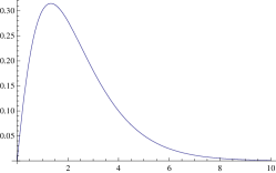
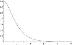
Figure 1: Plot of $\mathrm{d}{\ell}/\mathrm{d}u$ for massive scalars, fermions and vectors, respectively.

Third, we consider massive vector fields, with

$$\mathcal{L}_{v}=\frac{1}{4}W_{\mu\nu}^{2}+\frac{m^{2}}{2}W_{\mu}^{2},\qquad\mathrm{d}\mathcal{L}_{v}=m\mathrm{d}mW_{\mu}^{2},$$ (4.6)

where $W_{\mu\nu}\equiv\partial_{\mu}W_{\nu}-\partial_{\nu}W_{\mu}$. We have

$$\mathrm{d}\ell=2\pi^{2}\hat{x}^{4}m\mathrm{d}m\sqrt{\left(\langle W_{\mu}(\hat{x}_{v})\hskip 0.72229ptW_{\nu}(0)\rangle\right)^{2}},\qquad\langle W_{\mu}(x)\hskip 0.72229ptW_{\nu}(0)\rangle=\left(\delta_{\mu\nu}-\frac{\partial_{\mu}\partial_{\nu}}{m^{2}}\right)\left(\frac{m}{4\pi^{2}x}K_{1}^{2}(xm)\right),$$

where $x=\sqrt{x_{1}^{2}+x_{2}^{2}+x_{3}^{2}+x_{4}^{2}}$. The explicit formula of $\mathrm{d}\ell$ is an involved expression containing several Bessel functions, which we do not write here. It tends to infinity in the ultraviolet limit, which is expected, since a massive vector is singular there. Precisely,

$$\left.\mathrm{d}\ell\right|_{u\rightarrow 0}\sim 2\sqrt{3}\frac{\mathrm{d}u}{u}.$$

In the same limit the distance $d(m_{2},m_{1})$ tends to a finite constant if $m_{2}>m_{1}>0$:

$$\left.d(m_{2},m_{1})\right|_{\hat{x}\rightarrow 0}=2\sqrt{3}\ln\frac{m_{2}}{m_{1}}.$$

It tends to infinity with a logarithmic singularity when one mass tends to zero:

$$\left.d(m_{2},m_{1})\right|_{m_{1}\rightarrow 0}\sim-2\sqrt{3}\ln(m_{1}\hat{x}).$$

Finally, it tends to zero in the infrared limit for $m_{2}>m_{1}>0$.

If a symmetry is spontaneously broken by the non-vanishing vacuum expectation value $v$ of some scalar field $\varphi$, then the distance between the symmetry-violating theory and the symmetric surface is proportional to $\hat{v}=v\hat{x}=v/E$ and correctly tends to zero for energies $E\gg v$. For example, consider the $\varphi^{4}$-theory

$$\mathcal{L}=\frac{1}{2}(\partial_{\mu}\varphi)^{2}+\frac{\lambda}{4!}\varphi^{4}-\frac{m^{2}}{2}\varphi^{2}.$$

Expanding the scalar field around its expectation value $v$ we get

$$\mathcal{L}(\lambda,v)=\frac{1}{2}(\partial_{\mu}\eta)^{2}+\frac{\lambda}{4!}\eta^{4}+\frac{\lambda v}{3!}\eta^{3}+\frac{\lambda v^{2}}{3!}\eta^{2}\equiv\mathcal{L}(\lambda)+\mathrm{d}\mathcal{L}(\lambda,v).$$

For $v$ small the distance has the form

$$d_{v}=\hat{v}(t)f(\lambda(t)),$$

where $\hat{v}(t)=v(t)\hat{x}$ and $\lambda(t)$ are the running couplings, and $f$ is some function. When the energy $E=1/\hat{x}$ is much larger than $v$ (but smaller than the dynamical scale $\mu$, so that the perturbative expansion in $\lambda$ is still meaningful), the distance tends to zero and the symmetry is restored. At higher energies the theory behaves like an ordinary $\varphi^{4}$-theory.

5 Marginal Lorentz-violating deformations of massless free relativistic fields

In this section we calculate the distance in the case of the most general marginal CPT-invariant Lorentz-violating deformations of massless relativistic free fields. We study the effects of minimizations with respect to tangent and reparametrization-displacements. We also use our results to discuss a number of conventions.

In Minkowskian notation, we write the total Lagrangian

$$\mathcal{L}_{\text{LI}}+\mathrm{d}\mathcal{L}_{\text{LV}},$$

as the sum of the Lorentz-invariant free Lagrangian

$$\mathcal{L}_{\text{LI}}=\frac{1}{2}(\partial_{\mu}\varphi_{I})(\partial^{\mu}\varphi_{I})+\frac{i}{2}\bar{\psi}_{A}\accentset{\leftrightarrow}{\partial}{\!\!\!\!\hskip 1.1pt/}\psi_{A}-\frac{1}{4}F_{\mu\nu}^{G}F^{G\hskip 0.72229pt\mu\nu}$$ (5.1)

and the Lorentz-violating perturbation

$$\mathrm{d}\mathcal{L}_{\text{LV}}=\frac{1}{2}\mathrm{d}\epsilon_{IJ}^{\mu\nu}(\partial_{\mu}\varphi_{I})(\partial_{\nu}\varphi_{J})+\frac{i}{2}\mathrm{d}c_{AB}^{\mu\nu}\bar{\psi}_{A}\gamma_{\mu}\accentset{\leftrightarrow}{\partial}_{\nu}\psi_{B}-\frac{1}{4}\mathrm{d}k_{GH}^{\mu\nu\rho\sigma}F_{\mu\nu}^{G}F_{\rho\sigma}^{H}.$$ (5.2)

For the moment, we do not assume particular conditions on the coefficients $\mathrm{d}\epsilon_{IJ}^{\mu\nu}$, $\mathrm{d}c_{AB}^{\mu\nu}$ and $\mathrm{d}k_{GH}^{\mu\nu\rho\sigma}$, other than their obvious symmetry and Hermiticity properties. Summations over repeated indices are understood. The fermions are assumed to be chiral, although we do not need to specify the chirality of each $\psi_{A}$.

Applying definition (2.1) we easily find the infinitesimal squared distance

$$\mathrm{d}\ell^{2}=\sum_{\mu\nu=0}^{3}(\mathrm{d}\bar{\epsilon}_{IJ}^{\mu\nu})(\mathrm{d}\epsilon_{IJ}^{\mu\nu})+2\sum_{\mu\nu=0}^{3}|\mathrm{d}c_{sAB}^{\mu\nu}|^{2}+3\sum_{\mu\nu=0}^{3}|\mathrm{d}\bar{c}_{aAB}^{\mu\nu}|^{2}-\frac{1}{2}|\mathrm{trd}c_{AB}|^{2}+\sum_{\mu\nu\rho\sigma=0}^{3}(\mathrm{d}k_{GH}^{\mu\nu\rho\sigma})^{2},$$ (5.3)

where

$$\mathrm{d}c_{sAB}^{\mu\nu} = \frac{1}{2}(\mathrm{d}c_{AB}^{\mu\nu}+\mathrm{d}c_{AB}^{\nu\mu}),\qquad\mathrm{d}\bar{c}_{aAB}^{\mu\nu}=\frac{3^{-(\delta_{\mu 0}+\delta_{\nu 0})/2}}{2i}(\mathrm{d}c_{AB}^{\mu\nu}-\mathrm{d}c_{AB}^{\nu\mu}),$$

$$\mathrm{trd}c_{AB} = (\mathrm{d}c_{AB})_{\hskip 3.61371pt\mu}^{\mu},\qquad\qquad\qquad\mathrm{d}\bar{\epsilon}_{IJ}^{\mu\nu}=\frac{3^{\delta_{\mu 0}+\delta_{\nu 0}}}{4}\mathrm{d}\epsilon_{IJ}^{\mu\nu}.$$

When the sum over space- and time-indices is written explicitly we mean that indices are contracted with the Euclidean metric. It is easy to verify that the two chiralities give the same contributions, which is why we do not need to distinguish them explicitly.

Now we consider tangent and reparametrization-displacements. We minimize $\mathrm{d}\ell^{2}$ with respect to each of them separately, and then together. The tangent displacements are the Lorentz-invariant contributions to $\mathrm{d}\mathcal{L}_{\text{LV}}$, namely

$$\frac{1}{2}\mathrm{d}\eta_{IJ}(\partial_{\mu}\varphi_{I})(\partial^{\mu}\varphi_{J})+\frac{i}{2}\mathrm{d}\tau_{AB}(\bar{\psi}_{A}\accentset{\leftrightarrow}{\partial}{\!\!\!\!\hskip 1.1pt/}\psi_{B})-\frac{1}{4}\mathrm{d}\zeta_{GH}(F_{\mu\nu}^{G}F^{\mu\nu H})-\frac{1}{8}\mathrm{d}\tilde{\zeta}_{GH}\varepsilon^{\mu\nu\rho\sigma}(F_{\mu\nu}^{G}F_{\rho\sigma}^{H}).$$

These displacements do not move us away from the Lorentz surface. Minimizing (5.3) we obtain the conditions

$$(\mathrm{d}\bar{\epsilon}_{IJ})_{\hskip 4.33601pt\mu}^{\mu}=0,\qquad(\mathrm{d}k_{GH})_{\hskip 3.61371pt\hskip 3.61371pt\mu\nu}^{\mu\nu}=0,\qquad\varepsilon_{\mu\nu\rho\sigma}\mathrm{d}k_{GH}^{\mu\nu\rho\sigma}=0.$$ (5.4)

Observe that no conditions on the fermionic parameters $\mathrm{d}c_{AB}^{\mu\nu}$ are generated. The reason is that the Dirac Lagrangian is proportional to its own field equations.

Infinitesimal reparametrizations of the form

$$x^{\prime\hskip 0.72229pt\mu}=x^{\mu}+\mathrm{d}a_{\nu}^{\hskip 3.61371pt\mu}\hskip 0.72229ptx^{\nu},\qquad A_{\mu}^{\prime}=A_{\mu}-\mathrm{d}a_{\mu}^{\hskip 3.61371pt\nu}\hskip 0.72229ptA_{\nu},$$ (5.5)

generate another noticeable subsector of $\mathrm{d}\mathcal{L}_{\text{LV}}$. Minimizing with respect to these displacements we obtain the relations

$$\mathrm{d}C^{\mu\nu}-\frac{g^{\mu\nu}}{4}(\mathrm{d}C)_{\hskip 4.33601pt\alpha}^{\alpha}=0,\qquad(\mathrm{d}B)_{\hskip 4.33601pt\mu}^{\mu}=0,$$ (5.6)

where we have defined

$$\mathrm{d}C^{\mu\nu}\equiv\mathrm{d}c_{AA}^{\mu\nu}+\mathrm{d}B^{\mu\nu},\qquad\mathrm{d}B^{\mu\nu}\equiv\mathrm{d}\bar{\epsilon}_{II}^{\mu\nu}+2(\mathrm{d}k_{GG})_{\hskip 6.50403pt\hskip 6.50403pt\alpha}^{\mu\alpha\nu}.$$

Finally, if we minimize with respect to spinor reparametrizations

$$\psi_{A}\rightarrow\psi_{A}+i\omega_{AB}^{\mu\nu}\sigma_{\mu\nu}\psi_{B},$$ (5.7)

we obtain that the fermionic parameters must be symmetric,

$$\mathrm{d}c_{AB}^{\mu\nu}=\mathrm{d}c_{AB}^{\nu\mu}.$$ (5.8)

When we minimize with respect of all classes of displacements altogether, we obviously obtain both (5.4), (5.6) and (5.8). These conditions are Lorentz covariant in the absence of scalar fields. Note that the first two formulas of (5.4) imply the second of (5.6).

Now we further study the meaning of the minimization with respect to the various kinds of displacements in simple examples. Consider $N$ Lorentz-violating rotation-preserving massless scalars, and take the perturbed Lagrangian

$$\mathcal{L}_{2s}+\mathrm{d}\mathcal{L}_{2s}=\frac{1}{2}\sum_{I}(\partial_{\mu}\varphi_{I})(\partial^{\mu}\varphi_{I})-\sum_{I}\mathrm{d}\epsilon_{I}(\partial_{i}\varphi_{I})^{2}.$$ (5.9)

The naïve squared distance between the Lorentz violating theory and the Lorentz invariant one reads

$$\mathrm{d}\ell^{2}=2\pi^{4}\hat{x}^{8}\langle\mathrm{d}\mathcal{L}_{2s}(\hat{x}_{v})\mathrm{\hskip 0.72229ptd}\mathcal{L}_{2s}(0)\rangle=3\sum_{I}(\mathrm{d}\epsilon_{I})^{2}.$$

However, if all $\mathrm{d}\epsilon_{I}$’s are equal the theory can be still written in a manifestly Lorentz invariant form rescaling the space coordinates. Thus, we write $\mathrm{d}\epsilon_{I}=\mathrm{d}\tilde{\epsilon}_{I}+\mathrm{d}a$ and minimize $\mathrm{d}\ell$ with respect to $\mathrm{d}a$. We obtain

$$\mathrm{d}\ell_{r}^{2}=\sum_{IJ}(\mathrm{d}\tilde{\epsilon}_{I})\gamma_{IJ}(\mathrm{d}\tilde{\epsilon}_{J})=\frac{3}{N}\sum_{I<J}(\mathrm{d}\tilde{\epsilon}_{I}-\mathrm{d}\tilde{\epsilon}_{J})^{2}.$$

The entries of the reduced metric $\gamma_{IJ}$ are $3(1-1/N)$ on the diagonal and $-3/N$ elsewhere. At the minimum the Lagrangian reads

$$\mathcal{L}_{2s}+\mathrm{d}\mathcal{L}_{2s}=\frac{1}{2}\sum_{I}(\partial_{\mu}\varphi_{I})(\partial^{\mu}\varphi_{I})-\sum_{I}\mathrm{d}\tilde{\epsilon}_{I}(\partial_{i}\varphi_{I})^{2}+\frac{1}{N}\sum_{IJ}\mathrm{d}\tilde{\epsilon}_{I}(\partial_{i}\varphi_{J})^{2},$$

and satisfies the relations (5.6), which just read $\sum_{I}\mathrm{d}\epsilon_{I}=0$ in this particular case.

Now, take two fields and assume that one is massive and the other one is not:

$$\mathcal{L}_{2s}+\mathrm{d}\mathcal{L}_{2s}=\frac{1}{2}\sum_{I=1}^{2}(\partial_{\mu}\varphi_{I})(\partial^{\mu}\varphi_{I})-\frac{m^{2}}{2}\varphi_{1}^{2}-\sum_{I=1}^{2}\mathrm{d}\epsilon_{I}(\partial_{i}\varphi_{I})^{2}.$$ (5.10)

Then we have a squared distance of the form

$$\mathrm{d}\ell^{2}=A(\mathrm{d}\epsilon_{1})^{2}+B(\mathrm{d}\epsilon_{2})^{2},$$ (5.11)

with $A\neq B$. The minimization with respect to $\mathrm{d}a$ no longer satisfies relations (5.6), since now $\mathrm{d}\epsilon_{1}+\mathrm{d}\epsilon_{2}\neq 0$. Moreover, it introduces considerable complicacies, because the functions $A$ and $B$ depend on the energy scale, among the other things.

For this reason, sometimes it may not be convenient to minimize with respect to reparametrization-displacements. Then the ambiguities associated with reparametrizations can be eliminated by means of a prescription. This corresponds to define the distance choosing a cross section of the Lagrangian bundle, as shown in formula (2.7).

One example is to impose relations (5.6) by default. This prescription can be adopted in the most general Lorentz-violating theory, also when the parameters $\mathrm{d}\epsilon$, $\mathrm{d}c$ and $\mathrm{d}k$ are not infinitesimal.

If scalar fields are present, this prescription is not Lorentz covariant. When we consider theories that are infinitesimally close to Lorentz-invariant ones, we may want to adopt alternative Lorentz covariant prescriptions. One example is to set the trace of fermion coefficients to zero:

$$\mathrm{d}c_{AA}^{\mu\nu}=0.$$ (5.12)

This condition is sufficient to remove the ambiguity, while analogous conditions on the scalar or vector coefficients remove only part of it.

It is always advisable to minimize with respect to tangent displacements, since they correspond to movements on the Lorentz surface. However, sometimes we may want to adopt prescriptions also for tangent displacements. Doing so, we are not really calculating the distance from the Lorentz-violating theory to the Lorentz surface, but the distance from the Lorentz-violating theory to a particular point on the surface. Examples of Lorentz covariant prescriptions for tangent displacements are

$$(\mathrm{d}k_{GH})_{\quad\mu\nu}^{\mu\nu}=0,\qquad\varepsilon_{\mu\nu\rho\sigma}\mathrm{d}k_{GH}^{\mu\nu\rho\sigma}=0,\qquad(\mathrm{d}c_{AB})_{\hskip 3.61371pt\mu}^{\mu}=0,\qquad(\mathrm{d}\epsilon_{IJ})_{\hskip 3.61371pt\mu}^{\mu}=0.$$ (5.13)

The first two are also found from the minimization, but the other two are not.

6 Distance in Lorentz-violating QED

Now we calculate the distance between Lorentz violating theories and the Lorentz surface. Again, we assume, for simplicity, that CPT is preserved. First we calculate $\mathrm{d}\ell$ in the low-energy sector of Lorentz-violating QED. This means that we include the Lagrangian terms that are renormalizable by ordinary power counting. Later we consider the QED subsector of the Lorentz-violating Standard Model of [4, 5], which includes higher-dimensional operators that are renormalizable by weighted power counting. We also comment on the contributions of CPT-violating terms.

The low-energy Lagrangian of Lorentz-violating QED is $\mathcal{L}_{\text{LI}}+\mathrm{d}\mathcal{L}_{\text{LV}}$, where

$$\mathcal{L}_{\text{LI}} = -\frac{1}{4}F^{\mu\nu}F_{\mu\nu}+\frac{i}{2}\bar{\psi}\accentset{\leftrightarrow}{\not{D}}{\psi}-m\bar{\psi}\psi,$$

$$\mathrm{d}\mathcal{L}_{\text{LV}} = -\frac{1}{4}(k_{F})_{\mu\nu\rho\sigma}F^{\mu\nu}F^{\rho\sigma}+\frac{1}{2}\bar{\psi}\left(ic^{\mu\nu}\gamma_{\mu}\accentset{\leftrightarrow}{D}_{\nu}+id^{\mu\nu}\gamma_{5}\gamma_{\mu}\accentset{\leftrightarrow}{D}_{\nu}-H_{\mu\nu}\sigma^{\mu\nu}\right)\psi,$$

where $D_{\mu}=\partial_{\mu}+ieA_{\mu}$ is the covariant derivative. The parameters $k_{F}$ and $H_{\mu\nu}$ satisfy the symmetry properties

$$(k_{F})_{\mu\nu\rho\sigma}=(k_{F})_{\rho\sigma\mu\nu}=-(k_{F})_{\nu\mu\rho\sigma},\qquad H_{\nu\mu}=-H_{\mu\nu}.$$

For the moment, we do not assume other conditions on the parameters.

Since the Lorentz violating parameters are bound to have very small values, to a first approximation we can neglect the fine structure constant and work around the free-field limit of QED.

The distance does depend on the energy. At energies much smaller than the electron mass $m_{e}$ the electron contribution is negligible and we can work in the pure photon sector. At energies much greater than $m_{e}$ we can work in the massless limit. In both cases we can use the formulas of the previous section, possibly adding the contributions of relevant operators.

We minimize with respect to tangent displacements, and evaluate the distance both before and after the minimization with respect to the reparametrization-displacements (5.5).

Photon sector

In the photon sector formula (5.3) gives

$$\mathrm{d}\ell_{\gamma}^{2}=\sum_{\mu\nu\rho\sigma=0}^{3}(k_{F}^{\mu\nu\rho\sigma})^{2}.$$

Minimizing with respect to tangent displacements we obtain conditions (5.4), which here read

$$(k_{F})_{\quad\mu\nu}^{\mu\nu}=0,\qquad\varepsilon_{\mu\nu\rho\sigma}k_{F}^{\mu\nu\rho\sigma}=0.$$ (6.1)

These relations leave 19 independent entries, out of 21. It is common [9] to express the surviving entries in terms of three traceless symmetric matrices $\tilde{k}_{e+}$, $\tilde{k}_{e-}$ and $\tilde{k}_{o-}$, an antisymmetric matrix $\tilde{k}_{o+}$ and a scalar $\tilde{k}_{\mathrm{tr}}$. After some manipulations we find

$$\mathrm{d}\ell_{\gamma}^{2}=6\tilde{k}_{\mathrm{tr}}^{2}+2\sum_{ij}\left[(\tilde{k}_{e-}^{ij})^{2}+(\tilde{k}_{o-}^{ij})^{2}+(\tilde{k}_{e+}^{ij})^{2}+(\tilde{k}_{o+}^{ij})^{2}\right].$$ (6.2)

Three coefficients can be eliminated, because $\tilde{k}_{e+}$, $\tilde{k}_{e-}$ and $\tilde{k}_{o-}$ are traceless. The tabulated quantities [1] in the standard Sun-centered inertial reference frame are $(\tilde{k}^{11}-\tilde{k}^{22})_{e+,e-,o-}$ and $\tilde{k}_{e+,e-,o-}^{33}$. Rewriting the result in terms of these, we have

$$\mathrm{d}\ell_{\gamma}^{2} = (\tilde{k}_{e-}^{11}-\tilde{k}_{e-}^{22})^{2}+(\tilde{k}_{e+}^{11}-\tilde{k}_{e+}^{22})^{2}+(\tilde{k}_{o-}^{11}-\tilde{k}_{o-}^{22})^{2}+4\sum_{i<j}\left((\tilde{k}_{e-}^{ij})^{2}+(\tilde{k}_{e+}^{ij})^{2}+(\tilde{k}_{o-}^{ij})^{2}+(\tilde{k}_{o+}^{ij})^{2}\right)$$ (6.3)

$$+3(\tilde{k}_{e-}^{33})^{2}+3(\tilde{k}_{e+}^{33})^{2}+3(\tilde{k}_{o-}^{33})^{2}+6\tilde{k}_{\mathrm{tr}}^{2}.$$

We can now maximize (6.3) using the maximal sensitivities of ref. [1], Table III. The main contribution comes from the parameter that is measured with the smallest precision, which is $\tilde{k}_{o+}^{12}$. We obtain

$$\mathrm{d}\ell_{\gamma}\sim 2\tilde{k}_{o+}^{12}\leqslant 2\times 10^{-13}.$$ (6.4)

If we include the CPT-violating contributions we obtain something like

$$\mathrm{d}\ell_{\gamma\text{CPT}}\lesssim 2\times 10^{-13}\sqrt{1+f\times 10^{-58}(\widehat{x}\hskip 0.72229pt\mathrm{GeV})^{2}},$$

where $f$ is a calculable numerical factor of order 1. This formula shows that on the basis of present knowledge possible CPT-violating contributions can be neglected for wavelengths smaller than 10^-3 light years.

Formula (6.4) is the result obtained before minimizing with respect to the reparametrizations (5.5). Such a minimization gives, from (5.6), the additional condition

$$\tilde{k}^{\mu\nu}=0,$$ (6.5)

where

$$\tilde{k}^{\mu\nu}\equiv(k_{F})_{\hskip 3.61371pt\hskip 3.61371pt\hskip 4.33601pt\alpha}^{\mu\alpha\nu}.$$

It is easy to show that an alternative form of (6.2) is

$$\mathrm{d}\ell_{\gamma}^{2}=2\sum_{\mu,\nu=0}^{3}(\tilde{k}\,^{\mu\nu})^{2}+2\sum_{ij}\left[(\tilde{k}_{e+}^{ij})^{2}+(\tilde{k}_{o-}^{ij})^{2}\right].$$ (6.6)

Then equation (6.5) gives

$$\mathrm{d}\ell_{\gamma}\leqslant 6\times 10^{-32}.$$ (6.7)

This value is much smaller than (6.4), because reparametrizations allow us to cancel out all nonbirefringent parameters. This can be done only in the absence of other particles.

Electron sector

Now we consider the fermionic sector in the massless limit, where we can use the formulas of the previous section, provided we add the contributions of relevant operators.

Formula (5.3) and the $H$-contribution give

$$\mathrm{d}\ell_{e}^{2}=\sum_{\mu\nu=0}^{3}\left[4(c^{\mu\nu})^{2}+4(d^{\mu\nu})^{2}+\widehat{x}^{2}(H^{\mu\nu})^{2}\right]-(c_{\mu}^{\hskip 3.61371pt\mu})^{2}-(d_{\mu}^{\hskip 3.61371pt\mu})^{2},$$ (6.8)

plus terms proportional to the antisymmetric parts of $c^{\mu\nu}$ and $d^{\mu\nu}$. Minimizing with respect to the spinor reparametrizations (5.7) we get (5.8), which tells us that $c$ and $d$ are symmetric matrices. Moreover, the traces of $c$ and $d$ cancel out, so we assume that they vanish.

Maximizing (6.8) using the maximal sensitivities of ref. [1], Table II, for the electron, which is to date the only particle except the photon whose parameters are fully measured (in the CPT-even sector), we get

$$\mathrm{d}\ell_{e}\leqslant\sqrt{3\times 10^{-28}+5\times 10^{-39}(\widehat{x}\hskip 0.72229pt\mathrm{{GeV})^{2}}}\mathrm{.}$$ (6.9)

Since the zero-mass approximation is valid for energies greater than $m_{e}$, this result holds for $\widehat{x}\lesssim 1/m_{e}$. At energy $m_{e}$ we have

$$\mathrm{d}\ell_{e}\leqslant 2\times 10^{-14}.$$ (6.10)

Low-energy Lorentz-violating QED

At energies much greater than $m_{e}$ we can work in the massless limit. Formula (5.3) gives

$$\mathrm{d}\ell_{\text{QED}}^{2}=\sum_{\mu\nu\rho\sigma=0}^{3}(k_{F}^{\mu\nu\rho\sigma})^{2}+\sum_{\mu\nu=0}^{3}\left[4(c^{\mu\nu})^{2}+4(d^{\mu\nu})^{2}+\widehat{x}^{2}(H^{\mu\nu})^{2}\right]-(c_{\mu}^{\hskip 3.61371pt\mu})^{2}-(d_{\mu}^{\hskip 3.61371pt\mu})^{2},$$ (6.11)

plus contributions proportional to the antisymmetric parts of $c^{\mu\nu}$ and $d^{\mu\nu}$. As before, the traces of the matrices $c$ and $d$ do not contribute to the distance, so we assume that they vanish. Moreover, minimizing with respect to tangent-displacements and spinor reparametrizations, we get again (6.1) and that the matrices $c$ and $d$ are symmetric. In the end, the conditions we find coincide with the currently adopted conventions [3, 8].

The distance is just $\mathrm{d}\ell_{\text{QED}}=\sqrt{\mathrm{d}\ell_{\gamma}^{2}+\mathrm{d}\ell_{e}^{2}}$, where $\mathrm{d}\ell_{\gamma}$ and $\mathrm{d}\ell_{e}$ are given by (6.4) and (6.10), respectively. Since $\mathrm{d}\ell_{e}$ is smaller than $\mathrm{d}\ell_{\gamma}$ by one order of magnitude, we get $\mathrm{d}\ell_{\text{QED}}\sim 2\times 10^{-13}$. We recall that this result holds for $\widehat{x}\lesssim 1/m_{e}$. For $\widehat{x}\gtrsim 1/m_{e}$ we have instead (6.4).

These are the numerical values that we obtain before minimizing with respect to the reparametrizations (5.5). When we do minimize with respect to them, we get, from (5.6),

$$\tilde{k}^{\mu\nu}+c^{\mu\nu}=0.$$ (6.12)

We can derive this condition more directly as follows. Using (6.6), we can write

$$\mathrm{d}\ell_{\text{QED}}^{2}=2\sum_{\mu,\nu=0}^{3}(\tilde{k}\,^{\mu\nu})^{2}+2\sum_{ij}\left[(\tilde{k}_{e+}^{ij})^{2}+(\tilde{k}_{o-}^{ij})^{2}\right]+\sum_{\mu\nu=0}^{3}\left[4(c^{\mu\nu})^{2}+4(d^{\mu\nu})^{2}+\widehat{x}^{2}(H^{\mu\nu})^{2}\right].$$ (6.13)

Under reparametrizations (5.5) $\tilde{k}^{\mu\nu}\rightarrow\tilde{k}^{\mu\nu}-2a^{\mu\nu}-g^{\mu\nu}a_{\rho}^{\hskip 3.61371pt\rho}$. To preserve the first of (6.1), we take a traceless $a^{\mu\nu}$. Then the birefringent quantities $\tilde{k}_{e+}$ and $\tilde{k}_{o-}$ are invariant, while the polarization-independent quantities $\tilde{k}_{e-}$, $\tilde{k}_{o+}$ and $\tilde{k}_{\mathrm{tr}}$ are collected in the tensor $\tilde{k}^{\mu\nu}$. In the electron sector $c^{\mu\nu}\rightarrow c^{\mu\nu}-a^{\mu\nu}$ under (5.5), while $d^{\mu\nu}$ and $H^{\mu\nu}$ are invariant. Making the replacements in (6.13) and minimizing with respect to $a^{\mu\nu}$, we get

$$\mathrm{d}\ell_{\text{QED}}^{2}=\sum_{\mu\nu=0}^{3}\left[\frac{2}{3}(\tilde{k}^{\mu\nu}-2c^{\mu\nu})^{2}+4(d^{\mu\nu})^{2}+\widehat{x}^{2}(H^{\mu\nu})^{2}\right]+2(\tilde{k}_{e+}^{ij})^{2}+2(\tilde{k}_{o-}^{ij})^{2}.$$ (6.14)

We point out the appearance of the combination $\tilde{k}^{\mu\nu}-2c^{\mu\nu}$, which is indeed the one on which physical processes depend [10]. Formula (6.14) agrees with (6.12), because only $\tilde{k}^{\mu\nu}+c^{\mu\nu}=0$ turns (6.13) into (6.14).

We can now use the maximal sensitivities reported in ref. [1], Tables II and III, to give an upper bound on $\mathrm{d}\ell_{\text{QED}}$. The coefficients $\tilde{k}_{e+}$ and $\tilde{k}_{o-}$ are constrained to be smaller than $10^{-32}$, so we can ignore them. Again the only relevant terms are the ones that contain $\tilde{k}_{o+}^{12}$. We find

$$\mathrm{d}\ell_{\text{QED}}\leqslant\sqrt{10^{-26}+5\times 10^{-39}(\widehat{x}\hskip 0.72229pt\mathrm{{GeV})^{2}}}.$$

This formula holds for $\widehat{x}\lesssim 1/m_{e}$, where the second contribution under the square root is negligible, so we get

$$\mathrm{d}\ell_{\text{QED}}\leqslant\frac{2}{\sqrt{3}}\tilde{k}_{o+}^{12}\leqslant 10^{-13}.$$ (6.15)

For $\widehat{x}\gtrsim 1/m_{e}$ we have instead (6.7).

QED subsector of the high-energy-Lorentz-violating Standard Model

Now we calculate the distance in the QED subsector of the Lorentz-violating Standard Model of refs. [4, 5]. For simplicity, we assume that rotations are preserved, besides parity and CPT, and concentrate on the photon sector. We consider two choices for the total-derivative terms, and compare the results we obtain. In the next section the dependence on total-derivative terms is analysed in more detail.

We have seen that in general the distance can depend on the coordinate parametrization. In the previous sections we have eliminated this ambiguity minimizing with respect to reparametrization-displacements or choosing some prescriptions. In some cases Lorentz-violating theories eliminate the problem by themselves, because they already choose a preferred reference frame.

For example, the Lorentz-violating Standard Model of ref.s [4, 5] has a Lagrangian that contains higher space derivatives, to ensure renormalizability by weighted power counting. However, that Lagrangian does not contain higher time derivatives, to ensure perturbative unitarity. A reparametrization (5.5) spoils this structure unless $\mathrm{d}a_{0}^{\hskip 3.61371pti}\hskip 0.72229pt=0$. Moreover, it is assumed that there exists a preferred frame where the theory is invariant under spatial rotations. Then, if we want to preserve manifest rotational invariance we must also have $\mathrm{d}a_{i}^{\hskip 3.61371pt0}\hskip 0.72229pt=0$ and $\mathrm{d}a_{i}^{\hskip 3.61371ptj}\hskip 0.72229pt=\delta_{j}^{i}\mathrm{d}a$. In the end, only time- and space-rescalings survive.

We study the Lagrangians $\mathcal{L}_{\text{LI}}+\mathrm{d}\mathcal{L}_{\text{LV}}$ and $\mathcal{L}_{\text{LI}}+\mathrm{d}\mathcal{L}_{\text{LV}}^{\prime}$, where

$$\mathcal{L}_{\text{LI}}=-\frac{1+\delta_{1}}{4}F_{\mu\nu}F^{\mu\nu}$$

and

$$\mathrm{d}\mathcal{L}_{\text{LV}} = -\frac{\delta_{2}}{4}(F^{ij})^{2}+\frac{\tau_{1}}{4\Lambda_{L}^{2}}F^{ij}\partial_{k}^{2}F^{ij}-\frac{\tau_{0}}{4\Lambda_{L}^{4}}(\partial_{k}^{2}F^{ij})(\partial_{l}^{2}F^{ij}),$$

$$\mathrm{d}\mathcal{L}_{\text{LV}}^{\prime} = -\frac{\delta_{2}}{4}(F^{ij})^{2}-\frac{\tau_{1}}{4\Lambda_{L}^{2}}(\partial_{k}F^{ij})^{2}-\frac{\tau_{0}}{4\Lambda_{L}^{4}}(\partial_{k}\partial_{l}F^{ij})^{2}.$$ (6.16)

A $\delta_{1}$-variation is a tangent displacement. Time- and space-rescalings correspond to appropriate variations of $\delta_{1}$ and $\delta_{2}$. We minimize with respect to $\delta_{1}$ and keep $\delta_{2}$ as an independent coupling.

The two distances we find are

$$\mathrm{d}\ell_{\text{QED}}^{2} = \frac{3}{2}\delta_{2}^{2}+60\frac{\delta_{2}\tau_{1}}{\hat{\Lambda}_{L}^{2}}+1200\frac{\delta_{2}\tau_{0}}{\hat{\Lambda}_{L}^{4}}+1260\frac{\tau_{1}^{2}}{\hat{\Lambda}_{L}^{4}}+76800\frac{\tau_{0}\tau_{1}}{\hat{\Lambda}_{L}^{6}}+1876800\frac{\tau_{0}^{2}}{\hat{\Lambda}_{L}^{8}},$$

$$\mathrm{d}\ell_{\text{QED}}^{\prime\hskip 0.72229pt2} = \frac{3}{2}\delta_{2}^{2}-24\frac{\delta_{2}\tau_{1}}{\hat{\Lambda}_{L}^{2}}+480\frac{\delta_{2}\tau_{0}}{\hat{\Lambda}_{L}^{4}}+384\frac{\tau_{1}^{2}}{\hat{\Lambda}_{L}^{4}}-3840\frac{\tau_{0}\tau_{1}}{\hat{\Lambda}_{L}^{6}}+505920\frac{\tau_{0}^{2}}{\hat{\Lambda}_{L}^{8}},$$ (6.17)

respectively. We see that the two expressions have the same qualitative features. Either of them (or any other Lagrangian differing from $\mathrm{d}\mathcal{L}_{\text{LV}}$ and $\mathrm{d}\mathcal{L}_{\text{LV}}^{\prime}$ by total-derivative terms) can be used to define the distance.

At present the ratio $\tau_{0}/\Lambda_{L}^{4}$ is constrained to be smaller than $10^{-24}\mathrm{GeV}^{-4}$, while $|\tau_{1}|/\Lambda_{L}^{2}$ is smaller than $10^{-21}\mathrm{GeV}^{-2}$ [7]. With these values and $\delta_{2}=-2\tilde{k}_{\mathrm{tr}}$, $|\delta_{2}|\leqslant 2\times 10^{-14}$, we get from (6.17) the upper bounds

$$\mathrm{d}\ell_{\text{QED}}^{2} \leqslant 6\times 10^{-28}\left(1+2\times 10^{-6}q^{2}+4\times 10^{-8}q^{4}+10^{-13}q^{6}+3\times 10^{-15}q^{8}\right),$$

$$\mathrm{d}\ell_{\text{QED}}^{\prime\hskip 0.72229pt2} \leqslant 6\times 10^{-28}\left(1+8\times 10^{-7}q^{2}+2\times 10^{-8}q^{4}+6\times 10^{-15}q^{6}+8\times 10^{-16}q^{8}\right),$$ (6.18)

where $q=\hat{x}\mathrm{GeV}$. The formulas are valid as long as $\mathrm{d}\mathcal{L}_{\text{LV}}$ or $\mathrm{d}\mathcal{L}_{\text{LV}}^{\prime}$ are small, namely up to $10^{6}\mathrm{GeV}$. At this energy we find

$$\mathrm{d}\ell_{\text{QED}}^{2}\leqslant 2\times 10^{6},\qquad\mathrm{d}\ell_{\text{QED}}^{\prime\hskip 0.72229pt2}\leqslant 5\times 10^{5}.$$ (6.19)

Ignoring the $\tau_{0}$-term the resulting formulas are valid up to $10^{10}\mathrm{GeV}$, where they give

$$\mathrm{d}\ell_{\text{QED}}^{2}\leqslant 13,\qquad\mathrm{d}\ell_{\text{QED}}^{\prime\hskip 0.72229pt2}\leqslant 4\text{.}$$ (6.20)

These distances are large because at present the bounds on the parameters of higher-dimensional corrections are not so strong. In particular, formula (6.19) reflects the bound on $\tau_{0}$, while formula (6.20) reflects the bound on $\tau_{1}$.

Observe that the large numerical coefficients appearing in formulas (6.18) can be turned into coefficients of order one if we incorporate a factor 1/6 in $\Lambda_{L}$. This means that the Lorentz violation introduced by higher-derivative terms starts to become important at energies $E\sim\Lambda_{Lr}\equiv\Lambda_{L}/6$, rather than $E\sim\Lambda_{L}$, as naively suggested by the Lagrangians (6.16). In other physical quantities the effects of higher-dimensional operators may be enhanced even more.

CPT-violating quadratic corrections to the photon lagrangian carry odd powers of momentum. Normally they are relevant operators by weighted power counting, therefore in the ultraviolet limit their contributions to the distance are negligible with respect to some prevailing CPT-even contributions.

7 Coordinate changes, total derivatives and other dependencies

In section 4 we illustrated how the metric and the distance depend on the energy scale, and shown that such dependencies have physically reasonable behaviors. However, the metric depends on several less meaningful parameters, which may be introduced changing coordinates and adding total derivatives. Precisely, it does depend on the Lagrangian used to calculate it. In this section we illustrate these dependencies further more.

Theories that are perturbatively equivalent can be described by Lagrangians differing by total derivatives. Since the metric is based on the two-point function of the Lagrangian perturbation $\mathrm{d}\mathcal{L}$, a total-derivative perturbation can generate a non-vanishing distance. Let us consider free massive scalar fields again, but now rescale them by some factor $\mathrm{e}^{\Omega/2}$. We take the Lagrangian

$$\mathcal{L}_{\Omega}=\frac{\mathrm{e}^{\Omega}}{2}(\partial_{\mu}\varphi)^{2}+\mathrm{e}^{\Omega}\frac{m^{2}}{2}\varphi^{2}.$$

The difference $\mathcal{L}_{\Omega}-\mathcal{L}_{0}$ is not proportional to the field equations, so it does contribute to the distance. Now the two-parameter perturbation reads

$$\mathrm{d}\mathcal{L}_{\Omega}=\mathcal{L}_{\Omega}\mathrm{d}\Omega+\mathrm{e}^{\Omega}m\mathrm{d}m\hskip 0.72229pt\varphi^{2}$$

and the metric is

$$\left(\begin{tabular}[]{cc}$g_{mm}$&$g_{m\Omega}$\\ $g_{\Omega m}$&$g_{\Omega\Omega}$\end{tabular}\right)=2\pi^{4}\hat{x}^{8}\left(\begin{tabular}[]{cc}$\mathrm{e}^{2\Omega}m^{2}\langle\varphi^{2}(\hat{x}_{v})\hskip 0.72229pt\hskip 0.72229pt\varphi^{2}(0)\rangle$&$\mathrm{e}^{\Omega}m\langle\hskip 0.72229pt\varphi^{2}(\hat{x}_{v})\hskip 0.72229pt\mathcal{L}_{\Omega}(0)\rangle$\\ $\mathrm{e}^{\Omega}m\langle\mathcal{L}_{\Omega}(\hat{x}_{v})\hskip 0.72229pt\hskip 0.72229pt\varphi^{2}(0)\rangle$&$\langle\mathcal{L}_{\Omega}(\hat{x}_{v})\hskip 0.72229pt\mathcal{L}_{\Omega}(0)\rangle$\end{tabular}\right).$$ (7.1)

In this simple case the metric is $\Omega$-independent, which is important for the reason we explain below.

Consider an arbitrary trajectory $\Omega(m)$ from $m_{1}$ to $m_{2}$. The distance calculated along the path $\Omega(m)$ is

$$d[\Omega]=\int_{m_{1}}^{m_{2}}\mathrm{d}m\sqrt{g_{mm}+2g_{m\Omega}\Omega^{\prime}+g_{\Omega\Omega}\Omega^{\prime\hskip 0.72229pt2}}.$$ (7.2)

Since theories with different values of $\Omega$ are physically equivalent, the distance should not depend on the boundary values $\Omega(m_{1})$ and $\Omega(m_{2})$. A distance with such a property can be defined minimizing $d[\Omega]$ with respect to the paths $\Omega(m)$, with free boundary conditions. The minimization gives

$$\Omega^{\prime}=-\frac{g_{m\Omega}}{g_{\Omega\Omega}},$$ (7.3)

an orthogonality relation similar to the ones found before. Finally, the distance between two massive theories reads

$$d(m_{2},m_{1})=\int_{m_{1}}^{m_{2}}\mathrm{d}m\sqrt{g_{mm}-\frac{g_{m\Omega}^{2}}{g_{\Omega\Omega}}}.$$ (7.4)

This result can be easily generalized to the case of several massive scalars. If we take a unique overall rescaling factor $\mathrm{e}^{\Omega}$ the metric is still $\Omega$-independent. In that case, considering $m$ as a vector, we can easily prove that the distance obeys the triangle inequality

$$d(m_{3},m_{2})+d(m_{2},m_{1})\geqslant d(m_{3},m_{1}).$$ (7.5)

Indeed, since the metric is $\Omega$-independent, the minimizing trajectories $\Omega(m_{i},m_{j})$ connecting $m_{i}$ and $m_{j}$ can be freely translated. We can use a translation to join the endpoints of $\Omega(m_{3},m_{2})$ and $\Omega(m_{2},m_{1})$ at $m_{2}$, which gives a path $\bar{\Omega}(m)$ connecting $m_{1}$ with $m_{3}$. Thus, the right-hand side of (7.5) is not greater than the left-hand side, since it is obtained minimizing with respect to a set of paths that includes $\bar{\Omega}(m)$.

In the one-scalar case (7.4) gives an involved expression that we do not report here, but obviously the distance is smaller than (4.2). For example, the distance between a massive and a massless field in the infrared limit turns out to be

$$\left.d(m,0)\right|_{\hat{x}\rightarrow\infty}=0.482,$$ (7.6)

instead of 1.

Assume now that a problem (7.2) is given, where, however, the metric does depend on $\Omega$ (an explicit example is given below). Then the minimization with respect to paths $\Omega(m)$ with free boundary conditions gives the Euler equations plus the boundary conditions $g_{m\Omega}+g_{\Omega\Omega}\Omega^{\prime}=0$ at $m_{1}$ and $m_{2}$. The boundary conditions determine both $\Omega(m_{1})$ and $\Omega(m_{2})$, so it is impossible to paste the trajectories $\Omega(m_{3},m_{2})$ and $\Omega(m_{2},m_{1})$ at $m_{2}$ and prove the triangle inequality. If we want to eliminate the $\Omega$-arbitrariness and keep the triangle inequality we must choose a convention, for example demand that the kinetic term $\dot{\varphi}^{2}/2$ be normalized to one. Then the correct results are (4.2) and (4.3).

If we repeat the rescaling exercise for fermions, we still get (4.4) and (4.5), since the fermion rescaling generates a perturbation proportional to the field equations. In the case of massive vectors we find results similar to the ones of the scalar case.

Now we study how the distance depends on the coordinate frame in more detail. In formula (2.1) a time axis is chosen to apply reflection positivity. If the theory is Lorentz invariant, and expressed in manifestly Lorentz covariant form, the choice of time axis does not affect the distance. However, a Lorentz invariant theory can also be expressed in a form that is not manifestly Lorentz covariant. For example, we can make a coordinate transformation

$$x_{\mu}^{\prime}=(A^{-1})_{\mu\nu}x_{\nu},$$ (7.7)

$A$ being any real invertible matrix. Then the distance does depend on $A$. Explicitly, let us consider a scalar field with Lagrangian

$$\mathcal{L}_{B}=\frac{1}{2}B_{\mu\nu}\partial_{\mu}\varphi\partial_{\nu}\varphi+\frac{m^{2}}{2}\varphi^{2}.$$ (7.8)

This theory is equivalent to the relativistic scalar field after the replacement (7.7) plus

$$\varphi^{\prime}(x^{\prime})=\sqrt{\det A}\hskip 0.72229pt\varphi(x),$$ (7.9)

where $B=A^{2}$. We want to calculate the distance between two massive theories in the reference frame (7.8). We have

$$\mathrm{d}\mathcal{L}_{B}(x)=m\mathrm{d}m\hskip 0.72229pt\varphi^{2}(x)=\frac{m\mathrm{d}m}{\det A}\hskip 0.72229pt\varphi^{\prime\hskip 0.72229pt2}(x^{\prime}),$$

and in the primed frame we can use the formulas found above. We find

$$\mathrm{d}\ell=\pi^{2}\hat{x}^{4}\sqrt{2\langle\mathrm{d}\mathcal{L}_{B}(\hat{x}_{v})~{}\mathrm{d}\mathcal{L}_{B}(0)\rangle}=\frac{2\pi^{2}\hat{x}^{4}m\mathrm{d}m}{\det A}\hskip 0.72229pt\langle\varphi^{\prime}(\hat{x}_{v}^{\prime})~{}\varphi^{\prime}(0)\rangle,$$

where

$$(\hat{x}_{v}^{\prime})_{\mu}=(A^{-1})_{\mu\nu}(\hat{x}_{v})_{\nu}=(A^{-1})_{\mu 0}\hat{x},\qquad|\hat{x}_{v}^{\prime}|=\sqrt{(B^{-1})_{00}}\hat{x}.$$

We finally get

$$\mathrm{d}\ell=\frac{u^{\prime\hskip 0.72229pt2}\mathrm{d}u^{\prime}\hskip 0.72229ptK_{1}\left(u^{\prime}\right)}{2(B^{-1})_{00}^{2}\sqrt{\det B}}\hskip 0.72229pt,\qquad u^{\prime}=m\hat{x}\sqrt{(B^{-1})_{00}}.$$ (7.10)

With respect to (4.1), we just get rescaling factors, yet the formula shows that the distance does depend on the choice of coordinate frame. For example, the distance between a massive and a massless scalar field in the infrared limit is

$$\left.d(m,0)\right|_{\hat{x}\rightarrow\infty}=\frac{1}{(B^{-1})_{00}^{2}\sqrt{\det B}}.$$

If we minimize with respect to $B_{\mu\nu}$ we find zero. Thus, in general when we minimize with respect to the full set of Lagrangian formulations we get a trivial result. Instead, as explained in section 2, the minimization with respect to the Lagrangian formulation must be subject to constraints. Typically, it is sufficient to fix the form of one theory. If one theory is Lorentz invariant, it is sufficient to demand that it be formulated in a manifestly covariant form.

Instead of treating $B_{\mu\nu}$ as fixed matrix, we can consider deformations of both $B_{\mu\nu}$ and $m$. Using a matrix notation, we then have

$$\mathrm{d}\mathcal{L}_{B}(x)=(\partial\varphi)^{T}\frac{\mathrm{d}B}{2}\partial\varphi(x)+m\mathrm{d}m\hskip 0.72229pt\varphi^{2}(x)=\frac{1}{\det A}\left[(\partial^{\prime}\varphi^{\prime})^{T}A^{-1}\frac{\mathrm{d}B}{2}\hskip 0.72229ptA^{-1}\partial^{\prime}\varphi^{\prime}+m\mathrm{d}m\hskip 0.72229pt\varphi^{\prime\hskip 0.72229pt2}\right],$$

where $T$ denotes transposition. After some straightforward manipulations we obtain

$$\mathrm{d}\ell^{2}=\frac{u^{\prime\hskip 0.72229pt4}}{16(B^{-1})_{00}^{4}\det B}\left\{\mathrm{tr}\left[\mathrm{d}B\hskip 0.72229ptC\mathrm{d}B\hskip 0.72229ptC\right]+4u^{\prime\hskip 0.72229pt2}K_{2}^{\prime\hskip 0.72229pt2}\mathrm{tr}[\mathrm{d}B\hskip 0.72229pt\tilde{B}^{-1}]\frac{\mathrm{d}m}{m}+4u^{\prime\hskip 0.72229pt2}K_{1}^{\prime\hskip 0.72229pt2}\frac{(\mathrm{d}m)^{2}}{m^{2}}\right\}\hskip 0.72229pt,$$ (7.11)

where

$$\tilde{B}^{-1}=\frac{B^{-1}\mathds{1}_{00}B^{-1}}{(B^{-1})_{00}},\qquad C=K_{2}^{\prime}B^{-1}-u^{\prime}K_{3}^{\prime}\tilde{B}^{-1},\qquad K_{n}^{\prime}\equiv K_{n}(u^{\prime}),$$

and $\mathds{1}_{00}$ is the matrix with entries $(\mathds{1}_{00})_{\mu\nu}=\delta_{\mu 0}\delta_{\nu 0}$. Comparing (7.11) with (7.1), we see that now the metric does depend on $B$, while (7.1) did not depend on $\Omega$.

We should now minimize with respect to $B$, namely solve the corresponding Euler equations and boundary conditions. This is difficult to do, so here for illustrative purposes we just minimize $\mathrm{d}\ell^{2}$ with respect to the reparametrization-displacements $\delta\mathrm{d}B_{\mu\nu}$. We obtain

$$\mathrm{d}\ell=\frac{u^{\prime\hskip 0.72229pt3}}{2(B^{-1})_{00}^{2}\sqrt{\det B}}\frac{\mathrm{d}m}{m}\sqrt{K_{1}^{\prime\hskip 0.72229pt2}-\frac{u^{\prime\hskip 0.72229pt2}K_{2}^{\prime\hskip 0.72229pt4}}{(K_{2}^{\prime}-u^{\prime}K_{3}^{\prime}\hskip 0.72229pt)^{2}}}.$$ (7.12)

The dependence on $B$ is even more involved than in (7.10). Again, the minimum with respect to $B$ gives a trivial result. Setting $\sqrt{\det B}=(B^{-1})_{00}=1$ we get

$$\left.d(m,0)\right|_{\hat{x}\rightarrow\infty}=0.466,$$

which is even smaller than (7.6).

To summarize, if we do not minimize with respect to $B$ the ambiguity in the choice of $B$ survives. If we do minimize we get a trivial result. To obtain a non-trivial result, we must minimize with a suitable constraint. Generally, we lose the triangle inequality. In practice, after the constrained minimization the distance has the properties of a distance between surfaces, not the properties of a distance between points. Obviously the distance between surfaces does not obey a simple triangle inequality.

Observe that in principle we should consider not just the linear reparametrizations (7.7), but the most general curved reparametrizations, and minimize (with constraints) with respect to them. This is another reason why in several situations it may be more convenient to remove the ambiguities associated with coordinate reparametrizations and total derivatives by means of prescriptions.

At the same time, it is interesting to observe is that all definitions share the same qualitative properties. For example, plotting (7.12) we see that it has the same shape as the first of Fig. 1. Despite its unusual features, we do believe that the distance defined here has the good properties to quantify the amount of symmetry violations.

8 Conclusions

We have studied the distance between symmetry-violating quantum field theories and the surface of symmetric theories. If a symmetry is known to be violated in Nature, the distance measures how small, or large, the violation is. If a symmetry, such as Lorentz symmetry, is not known to be violated in Nature, then, using experimental bounds on the parameters of the violation, the distance can be useful to quantify how precise the symmetry is at present. We stress that although at the Lagrangian level an explicit symmetry violation is in general described by a large number of independent parameters, the symmetry violation per se is actually governed by a single quantity, such as the distance we have studied here.

Our results can be applied to any symmetry, and also to study the distance between any pair or sets of theories. Here our main interest was to measure the current precision of Lorentz symmetry. We have focused on the QED subsector, first at low energies and later including higher-dimensional operators.

The distance has a number of interesting properties, but also unusual features. For example, it depends on total derivatives and coordinate parametrizations. In general, unwanted dependencies can be eliminated minimizing with respect to the parameters associated with them, but sometimes this procedure introduces more complicacies. Then it may be preferable to choose prescriptions. We have shown that in the massless limit of QED, the minimization gives constraints that coincide with the conventions currently used in the literature.

Acknowledgements

D.Anselmi wishes to thank Xinmin Zhang and the Institute of High Energy Physics of the Chinese Academy of Sciences, Beijing, for hospitality. D.Anselmi is supported by the Chinese Academy of Sciences, grant No. 2010T2J01.

Appendix: RG invariance of the distance

In this appendix we prove that the infinitesimal distances (2.5) and (3.8) are renormalization-group invariant. Although strictly speaking the argument we give applies to theories that are renormalizable by ordinary power counting, it can be immediately generalized to theories that are renormalizable by weighted power counting [6], once the dimensions of parameters and operators are replaced with their weights. Then $\mathrm{d}\ell^{2}$ is invariant along the “weighted” RG flow [6].

We start from (2.5). The renormalization-group equations give, in matrix notation,

$$G(t,\hat{\lambda})=z^{-1}(t)\hskip 0.72229ptG(0,\hat{\lambda}(t))\hskip 0.72229pt(z^{-1}(t))^{\dagger}.$$

The running renormalization constants read

$$z(t)=1+\sum_{k=1}^{\infty}(-1)^{k}\int_{0}^{t}\mathrm{d}t_{1}\int_{0}^{t_{1}}\mathrm{d}t_{2}\cdots\int_{0}^{t_{k-1}}\mathrm{d}t_{k}\ \gamma(t_{1})\ \cdots\ \gamma(t_{k-1})\ \gamma(t_{k})$$

and $\gamma(t)$ stands for $\gamma(\hat{\lambda}(t))$, where

$$\gamma_{IJ}=Z_{IK}^{-1}\frac{\mathrm{d}Z_{KJ}}{\mathrm{d}\ln\mu},\qquad\mathcal{O}_{I\mathrm{B}}=Z_{IJ}\mathcal{O}_{J},$$

the subscript B denoting bare quantities.

The running $\mathrm{d}\lambda$-parameters are $\mathrm{d}\hat{\lambda}(t)=\mathrm{d}\hat{\lambda}\hskip 0.72229ptz^{-1}(t)$, so we can express the infinitesimal length by means of the manifestly RG invariant formula

$$\mathrm{d}\ell=\sqrt{\mathrm{d}\hat{\lambda}^{I}(t)\hskip 0.72229ptG_{IJ}(0,\hat{\lambda}(t))\hskip 0.72229pt\mathrm{d}\hat{\lambda}^{J*}(t)}.$$

Observe that the runnings of $\hat{\lambda}$ and $\mathrm{d}\hat{\lambda}$ are related by the formula $\beta_{\mathrm{d}\lambda}^{\hskip 3.61371ptI}=\mathrm{d}\lambda^{J}(\partial\beta^{I}/\partial\lambda^{J})$, where $\beta^{I}$ is the beta function of $\lambda^{I}$. This can be proved shifting $\lambda$ by $\mathrm{d}\lambda$ in $\mu\mathrm{d}\lambda^{I}/\mathrm{d}\mu=\beta^{I}(\lambda)$.

The proof of RG-invariance can be extended to (3.8), where the metric is replaced by the reduced metric, obtained minimizing with respect to the displacements $\xi^{a}$ tangent to the Lorentz surface. First observe that when the Lorentz-violating parameters $\zeta^{i}$ identically vanish the theory is consistently renormalizable, because it is Lorentz invariant. This implies that the renormalization constants $Z_{ai}$ vanish, so $Z_{IJ}$ is block triangular. Using this fact, it is easy to prove that

$$\gamma_{ij}(t,\hat{\alpha})=z_{ik}^{-1}(t)\hskip 0.72229pt\gamma_{km}(0,\hat{\alpha}(t))\hskip 0.72229ptz_{jm}^{-1*}(t),$$

so finally the distance (3.8) depends only on the running couplings $\hat{\zeta}^{i}(t)=\hat{\zeta}^{j}z_{ji}^{-1}(t)$:

$$d_{L}(t,\hat{\zeta})=\sqrt{\hat{\zeta}^{i}\gamma_{ij}(t,\hat{\alpha})\hat{\zeta}^{*j}}=\sqrt{\hat{\zeta}^{i}(t)\hskip 0.72229pt\gamma_{ij}(0,\hat{\alpha}(t))\hskip 0.72229pt\hat{\zeta}^{*j}(t)}=d_{L}(0,\hat{\zeta}(t)).$$

References

• [1] V.A. Kostelecký and N. Russell, Data tables for Lorentz and CTP violation, Rev. Mod. Phys. 83 (2011) 11 and arXiv:0801.0287 [hep-ph].
• [2] A. B. Zamolodchikov, Irreversibility of the Flux of the Renormalization Group in a 2D Field Theory, JETP Lett. 43, 730 (1986).
• [3] D. Colladay and V.A. Kostelecký, Lorentz-violating extension of the Standard Model, Phys. Rev. D58 (1998) 116002 and arXiv:hep-ph/9809521.
• [4] D. Anselmi, Weighted power counting, neutrino masses and Lorentz violating extensions of the Standard Model, Phys. Rev. D 79 (2009) 025017 and arXiv:0808.3475 [hep-ph].
• [5] D. Anselmi, Standard Model without elementary scalars and high-energy Lorentz violation, Eur. Phys. J. C 65 (2010) 523 and arXiv:0904.1849 [hep-ph].
• [6] D. Anselmi and M. Halat, Renormalization of Lorentz violating theories, Phys. Rev. D 76 (2007) 125011 and arXiv:0707.2480 [hep-th].
• [7] V.A. Kostelecký and M. Mewes, Electrodynamics with Lorentz-violating operators of arbitrary dimension, Phys. Rev. D 80 (2009) 015020 and arXiv:0905.0031 [hep-ph].
• [8] V.A. Kostelecký, C.D. Lane and A.G.M. Pickering, One-loop renormalization of Lorentz-violating electrodynamics, Phys. Rev. D 65 (2002) 056006 and arXiv:hep-th/0111123.
• [9] V.A. Kostelecký and M. Mewes, Signals for Lorentz violation in electrodynamics, Phys. Rev. D 66 (2002) 056005 and arXiv:hep-ph/0205211.
• [10] See for example M.A. Hohensee, R. Lehnert, D.F. Phillips and R.L. Walsworth, Limits on isotropic Lorentz violation in QED from collider physics, Phys. Rev. D 80 (2009) 036010 and arXiv:0809.3442 [hep-ph].