Cubical Cohomology Ring of 3D Pictures
Abstract
Cohomology and cohomology ring of three-dimensional (3D) objects are topological invariants that characterize holes and their relations. Cohomology ring has been traditionally computed on simplicial complexes. Nevertheless, cubical complexes deal directly with the voxels in 3D images, no additional triangulation is necessary, facilitating efficient algorithms for the computation of topological invariants in the image context. In this paper, we present formulas to directly compute the cohomology ring of 3D cubical complexes without making use of any additional triangulation. Starting from a cubical complex that represents a 3D binary-valued digital picture whose foreground has one connected component, we compute first the cohomological information on the boundary of the object, by an incremental technique; then, using a face reduction algorithm, we compute it on the whole object; finally, applying the mentioned formulas, the cohomology ring is computed from such information.
Keywords: Cohomology ring; cubical complexes; 3D digital images.
url]http://www.personal.us.es/rogodi url]http://ma1.eii.us.es/miembros/majiro url]http://ma1.eii.us.es/miembros/medrano
1 Introduction
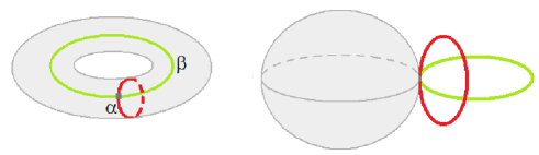
Many computer application areas involve topological methods which usually mean a significant reduction in the amount of data. Homology is an algorithmically computable topological invariant that characterizes an object by its “holes” (in any dimension). Informally, holes of a 3D-object are its connected components in dim. , its tunnels in dim. and its cavities in dim. . Cohomology is a topological invariant obtained by an algebraic duality of the notion of homology. Although the formal definition of cohomology is motivated primarily by algebraic considerations, homology and cohomology of 3D objects are isomorphic, that is, they provide the same topological information. Nevertheless, cohomology has an additional ring structure provided by the cup product (denoted by ). The cup product can be seen as the way the holes obtained in homology are related to each other. For example, think of the torus, and the wedge sum of two loops and a -sphere. Both objects have two tunnels and one cavity; but the cavity () of the first object can be decomposed in the product of the two tunnels ( and ), that is, ; the cavity of the second object cannot (see Fig. 1). This information would contribute to a better understanding of the degree of topological complexity of the analyzed digital object, and would shed light on its geometric features.
In [4, 5], a method for computing the cohomology ring of 3D binary digital images is stated. In those works, the cohomology ring computation is performed over the (unique) simplicial complex associated to the digital binary-valued picture using the -adjacency. However, one could assert that a more natural combinatorial structure when dealing with 3D digital images is the one provided by cubical complexes. One way to compute the cohomology ring of a cubical complex is to convert it into a simplicial complex by subdividing each cell and applying the known formulas for computing the cohomology ring of . In this paper, we present formulas to directly compute the cohomology ring of 3D cubical complexes without making use of additional triangulations. Besides, we describe a strategy to tackle the cohomology ring computation on a 3D binary-valued digital picture. This paper extends a preliminary version (see [2]).
The paper is organized as follows. In Section 2, we recall the concept of AT-model and extend it to general polyhedral cell complexes; given the AT-model for a polyhedral cell complex, we give the formulas of a new AT-model obtained after a subdivision; this result will be the key to prove the validity of the formulas of the cohomology ring of cubical complexes. In Section 3, formulas for computing the cohomology ring of 3D cubical complexes are established. Section 4 is devoted to describe the process to obtain an AT-model of a 3D digital image that provides the ingredients for the cohomology ring computation. Finally, some conclusions and plans for future are drawn in Section 5.
2 AT-models for Polyhedral Cell Complexes
In this section, we recall first the concept of AT-model (see [4, 5]) for a cell complex, which consists of an algebraic set of data that provides homological information. Given the AT-model for a polyhedral cell complex, we show the formulas of a new AT-model obtained after a subdivision; this result will be the key for the formulas of the cohomology ring of cubical complexes in the next section.
Since we are working with objects embedded in , the homology groups are torsion-free [1, ch.10], so computing homology over a field is enough to characterize shapes [11, p. 332]. This fact, together with the isomorphism (over any field) between the homology and cohomology groups [11, p. 320], enables us to consider as the ground ring throughout the paper.
A polyhedral cell complex in , is given by a finite collection of cells which are convex polytopes (vertices, edges, polygons and polyhedra), together with all their faces and such that the intersection between two of them is either empty or a face of each of them. A proper face of is a face of whose dimension is strictly less than the one of . A facet of is a proper face of of maximal dimension. A maximal cell of is a cell of which is not a proper face of any other cell of . Observe that if the cells of are -simplices, is a simplicial complex (see [11]); in the case that the cells of are -cubes, then is a cubical complex (see [9]). A -cell of either a simplicial complex or a cubical complex can be denoted by the list of its vertices.
For any graded set , one can consider formal sums of elements of , which are called -chains, and which form abelian groups with respect to the component-wise addition (mod ). These groups are called -chain groups and denoted by . The collection of all the chain groups associated to is denoted by and called also chain group, for simplicity. Let be the elements of for a fixed . Given two -chains and , where for , the expression refers to . For example, fixed and , the expression is and is if and otherwise.
The polyhedral chain complex associated to the polyhedral cell complex is the collection where:
-
(a)
each is the corresponding chain group generated by the -cells of ;
-
(b)
the boundary operator connects two immediate dimensions. The boundary of a -cell is the formal sum of all its facets. It is extended to -chains by linearity.
For example, consider a triangle with vertices , , . The boundary of the triangle is the formal sum of its edges, that is, .
Given a polyhedral cell complex , an algebraic-topological model (AT-model [4, 5]) for is a set of data , where is a graded subset of and are three families of maps , and , such that, for each :
-
(1)
, , , ;
-
(2)
, , .
As a result, the chain group is isomorphic to the homology (and to the cohomology) of . In particular, the number of vertices of coincides with the number of connected components of , the number of edges of with the number of tunnels of and the number of -cells of with the number of cavities of . Fixed , for each , is a representative cycle of a homology generator of dim. . Define an homomorphism such that if is a -cell of then
Then, is a representative cocycle of a cohomology generator of dim. . An isomorphism between and the homology (resp. cohomology) of maps each to the homology class represented by (resp. the cohomology class represented by ) (see [4, 5]).
a) b) c)
From now on, we will omit subscripts on behalf of simplicity.
Example 2.1
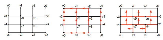
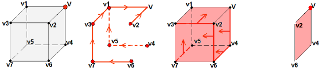
Let be an abstract cubical representation of the hollow torus given in Fig. 2. An AT-model for is the set of data given in the following table:
| , | ||||
| , | ||||
| , | ||||
| any edge | ||||
| any square |
where ; ; ; ; ; is the only path in from to in Fig. 2.b (for example, ); given an edge of , is the sum of the squares that correspond to the path starting from and following the arrows in Fig. 2.c (for example, ); representative cycles of homology generators are the vertex , the tunnels and and the cavity which is the sum of the squares of .
An algorithm for computing AT-models for polyhedral cell complexes appears for example in [4, 5]. In fact, in those papers, the algorithm is designed for simplicial complexes but the adaptation to polyhedral cell complexes is straightforward. That algorithm runs in time where is the number of cells of the given polyhedral cell complex. If an AT-model for a polyhedral cell complex is computed using that algorithm then it is also satisfied that if then and .
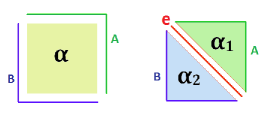
Let be a polyhedral cell complex. Fixed , we say that a -cell is subdivided into two new -cells and by a new -cell (see, for example, Fig. 3) if:
-
(a)
is a facet of and ;
-
(b)
;
-
(c)
.
The following lemma establishes how to obtain a new AT-model for after subdividing by a -cell a -cell of into two new -cells and . This result will be used to prove the equivalence between the new formula to compute the cup product on cubical complexes and the classical one on simplicial complexes.
Lemma 2.2
Let be an AT-model for a polyhedral cell complex computed using the algorithm given in [4, 5]. Let be a -cell, which is subdivided into two -cells and by a new -cell . Let if , and otherwise; ; and the boundary operator of given by: for any . Denote by , and by . Then, the set is an AT-model for , where , and are given by:
-
1.
;
, for any ; -
2.
, for any ; -
3.
If , ;
, for any .
ProofWe have to check that is an AT-model for . We will only check that and . The rest of the conditions are left to the reader.
Let , , and .
-
1.
:
If ; .
-
2.
:
.
(recall that since in an AT-model).
Besides,
Observe that , given by if and for any , is a chain-group isomorphism.
3 3D Cubical Cohomology Ring
In [12, 9], the authors consider cubical complexes as the geometric building blocks to compute the homology of digital images. In this section, we adapt to the cubical setting, the method developed in [4, 5] for computing the simplicial cohomology ring of 3D binary-valued digital pictures. We must mention [14, 10] as related works dealing with the cup product on cubical chain complexes in a theoretical context.
Since we are working with objects embedding in , it is satisfied that homology and cohomology are isomorphic. However, cohomology has the advantage over homology of having an additional ring structure given by the cup product, that is a topological invariant. This product provides information about the relationship between the generators of (co)homology, that enables to discriminate, for instance, pairs of cycles in different contexts, as in Fig. 1. Notice that, in 3D, the only non-trivial cup products are those corresponding to elements of cohomology of dim. . If the cup product of two elements of cohomology of dim. is not zero, then it is a sum of elements of cohomology of dim. . Recall that given an AT-model for a polyhedral cell complex , it is satisfied that is isomorphic to the homology and to the cohomology of .
3.1 Cohomology Ring of Simplicial Complexes
We recall now how the cup product is defined in the simplicial setting using AT-models:
Definition 3.1
Observe that for each , is a sum of -simplices representing one cavity. Then, is a sum of s and s over whose result is or . Therefore, is a sum of -simplices of of dim. , representing the cavities obtained by “multiplying” the two representative cycles and (think of the two tunnels of a hollow torus).
It is known that two objects with non-isomorphic cohomology rings, are not topologically equivalent (more precisely, they are not homotopic) [11]. To use the information of the cohomology ring for this aim, one can construct both matrices and collecting the results of the cup product of cohomology classes of dim. of each object, if the rank of and are different, then we can assert that both objects are not homotopic (see [5]).
3.2 Cohomology Ring of Cubical Complexes
Now, let be a cubical complex. Our aim is to obtain a direct formula for the cup product on without making use of any triangulation.
Suppose that the vertices of are labeled in a way that:
-
(P1)
Each square of with vertices has the edges , , and in its boundary.
For example, a cubical complex whose set of vertices is a subset of (the set of points with integer coordinates in 3D space ) with vertices labeled using the lexicographical order, satisfies P1.
Definition 3.2
Let be a cubical complex satisfying P1 and an AT-model for . Let be the set of squares of and let and be two edges of . The cup product of and is
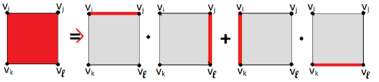
where on a square with vertices (see Fig. 4) is:
and is extended to -chains (sums of square) by linearity.
For simplicity, we sometimes use the notations for , and analogously for the simplicial cup product.
Example 3.1
Let be an abstract cubical representation of the hollow torus given in Fig. 2. Consider the AT-model for , given in Example 2.1. Recall that ; and , , and is the sum of the squares of , representing the connected component, the two tunnels and the cavity.
Apply the formula given in Def. 3.2 in order to obtain the cup product of and in :
then, . Recall that is the square in representing the cavity of the hollow torus. Therefore, the product of the two tunnels of the hollow torus is the cavity.
The following theorem shows the validity of the definition of (Def. 3.2). That is, it is stated that we obtain the same result by applying the formula of Def. 3.2 to compute the cup product on the cubical complex, than making first a triangulation in order to obtain a simplicial complex, and applying the classical definition of the cup product given in Def. 3.1, afterwards.
Consider successive subdivisions of each cube of a given cubical complex until each one is converted in six tetrahedra, and such that each square of is subdivided by the edge (see Fig. 5.d). Let us denote this resulting simplicial complex by . Observe that with this particular subdivision, if is a -simplex of , with , obtained by a subdivision of a square of , then and will correspond to edges in .
Theorem 3.1
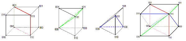
a) b) c) d)
ProofObserve that since and are edges of , then , that is, and . Observe also that on any edge since .
We have to prove that .
Let . Let and be the two triangles obtained after subdividing by the edge . Remember that and . Notice that coincides with if we replace by in the expression of . Therefore, it is enough to prove that :
This concludes the proof.
4 Cubical Cohomology Ring of 3D Digital Pictures
In this section, we develop the main bulk of the paper: beginning from a cubical complex that represents a 3D binary digital picture whose foreground has one connected component, first we compute an AT-model for the boundary of the object; then, having in mind that the homology of contains the homology of , we obtain an AT-model for with the representative cycles of homology generators lying in ; finally, applying the formula given in Section 3, the cohomology ring is computed from such an AT-model.
4.1 From Digital Pictures to Cubical Complexes
Each point of can be identified with a unit cube (called voxel) centered at this point, with facets parallel to the coordinate planes. This gives us an intuitive and simple correspondence between points in and voxels in .
Consider a 3D binary digital picture , where (the foreground) is finite, having as the underlying grid and fixing the -adjacency for the points of and the -adjacency for the points of (the background). We say that a voxel is in the boundary of if (i.e., if the point of identified with is in ) and has a -neighbor in .
Take the cubical complex for whose elements are the unit cubes (voxels) centered at the points of together with all their faces. Observe that this cubical complex with vertices labeled by the corresponding cartesian coordinates and considering the lexicographical order, satisfies (P1) (see page (P1)).
Without lack of generality, we consider that the foreground is connected.
The elements of are all the squares of which are shared by a voxel of and a voxel of together with all their faces.
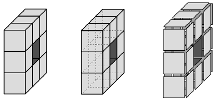
a) b) c)
4.2 AT-model for
Our interest now is to adapt the incremental algorithm for computing an AT-model given in [4, 5] to the particular complex .
First, consider the set of edges and vertices of as a graph and compute a spanning forest . Let be the trees of corresponding to the connected components of . Fixed , , take a vertex of and consider it as the root of .
Computing an AT-model for .
| Input: | The complex , |
| the set of trees of a spanning forest of , | |
| the set of roots of the trees of . |
-
1.
Initialize for any ; , , for some , . For to do From to the height of do For each vertex at level , and edge linking with its parent do , , . -
2.
While there are edges in do If there is a square with exactly one edge in its boundary do , , , . Else take an edge then , . -
3.
While there is a square in do . If then . Else take an edge in then . For each edge in do , , . -
4.
For each do .
| Output: the AT-model for . |
The auxiliary set is defined to indicate the cells which have already been used. In Step 1, neither the vertices nor the edges of create cycles except for the root . In Step 3, if a square has edges in its boundary that created cycles in a previous step, then one of these cycles is destroyed. Otherwise, this square creates a new cycle (a cavity). In the last step, the representative cycles of homology generators are computed.
Observe that all the steps of Alg. 4.2 are quadratic in the number of elements of (worse case complexity) except for the last part of Step 3 which is cubic in the number of edges of .
Example 4.1
The AT-model of a hollow cube (see Fig. 7) is:
| Step 1 | |||||
| , | |||||
| Step 2 | Any edge | 0 | |||
| Step 3 |
where is the only path in from to ; is the square at which the arrow corresponding to an edge in Fig. 7.c points, except for which is ; and is the sum of the six squares of .
a) b) c) d)
4.3 AT-model for
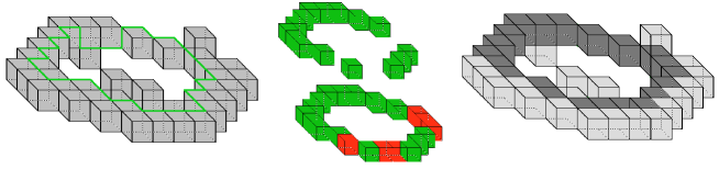
Now, we use a face reduction technique (see, for example, [3, 9, 13]) in order to obtain a cell complex such that homology, cohomology and cohomology ring of coincide with that of , and such that the cells of are also cells of .
Face Reduction Process.
| Input: A cubical complex . Initially, . | ||
| While | there exist such that is in do | |
| For | each cell such that is in do | |
| redefine as . | ||
| Remove and from the current ; | ||
| Output: the cell complex . |
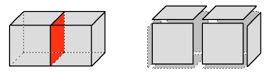
a) b)
Observe that after the face reduction process, we obtain a cell complex with the same topological information as but with much less cells. Now, starting from an AT model for , compute an AT-model for adding the cells of incrementally as follows:
AT-model for .
| Input: | An AT-model for : and the cells | ||
| of ordered by increasing dimension. | |||
| Initially, | , , for each ; | ||
| , , for each ; . | |||
| For | to do | ||
| take | a cell, , of , then | ||
| , | |||
| For | to do | ||
| Output: the AT-model for . |
Observe that in the algorithm, a cycle is never created because the cycles of are also cycles of . Therefore, when a cell of is added, then is never null and therefore a class of homology is always eliminated (that is, a cell of is removed from ). Alg. 4.3 is , where is the number of cells of (worst case complexity).
a) b) c)
4.4 From Cubical Complexes to Digital Pictures
Now, given a digital picture , suppose that we have computed an AT-model for , following the steps given in Subsections 4.1, 4.2 and 4.3. For each in , is a representative cycle of a homology generator of and, therefore, of , since the homology of and coincide and the representative cycles are in . Recall that if is a vertex, then is a vertex representing a connected component; if is an edge, then is a sum of edges representing a tunnel; and if is a square, then is a sum of squares representing a cavity.
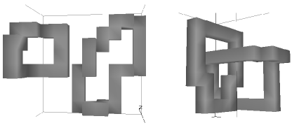
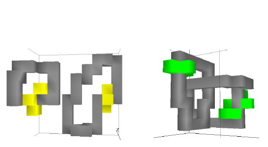
Given a representative cycle of a homology generator, our aim in this subsection is to draw the equivalent cycle in the picture .
First, if is a vertex then, is a face of a square in . This square is shared by a voxel of and a voxel of . Then, associate the voxel to the vertex .
Second, if is a sum of edges, suppose that is a simple cycle (if not, it can always be decomposed in simple ones). Visit all the edges of the cycle in order. If an edge, , and the next edge, , are facets of a square , then associate the single voxel of which has in its boundary, to the edges and . After that, visit all the edges that have not been associated to any voxel. If a voxel is associated with the next edge of the current one, , and there is a voxel having in its boundary, such that is in the boundary of and and are -neighbor, then associate to . If not, look at the previous edge and do the same procedure.
a) b)
If not, take any voxel of that contains , having a -neighbor voxel in .
Finally, if is a sum of squares, associate, to each square , the single voxel of which has in its boundary.
4.5 Cohomology ring of
Given a digital picture , its associated cubical complex and having computed an AT-model for , the last step of the process is the computation of the cohomology ring. This can be performed using the formula for the cubical cup product given in Def. 3.2.
Example 4.2
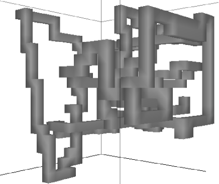
This example shows an application of to discriminate different embeddings of the same object. Consider the cubical complex (resp. ) associated to a digital picture where the set consists in two once-linked “circles” (resp. two unlinked “circles”). See Fig. 10. Both complexes have two tunnels and no cavities, so these properties are not able to distinguish them.
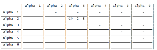
Now, denote by and , the cubical complexes associated to the background of and (white voxels of Fig. 10). Compute an AT-model for , and its cohmology ring, for . We obtain that the multiplication table for the cup product on is null whereas on is not (see Fig. 11). This fact allows us to assert that the two complexes and are not topologically equivalent.
Example 4.3
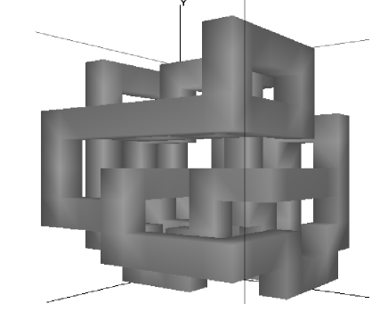
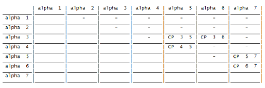
Consider the picture in Fig. 12. The cubical complex associated to the white voxels of the picture has connected component, tunnels and cavities. The cup product is trivial for any two pairs of homology classes except for two tunnels named as and wich is the sum of two of the three cavities (see Fig. 12).
Example 4.4
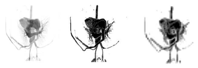
MRA of chest showing the heart and great vessels.
a) b) c)
Originally it was a stack of 14 gray-scale digital images in DICOM format, each one of size 320x320. This 2D stack can be see as the 3D digital image “chest” of dimensions 320x320x14 (see Fig. 14.a). After a binary process, we obtain the picture in Fig 14.b). “resized” 80x80x28
Let be the cubical complex that represents , let be
5 Conclusions and Future Work
In this paper we present formulas to directly compute the cohomology ring of 3D cubical complexes and develop a method for the computation on 3D binary-valued pictures. This computation on cubical complexes can be regarded as a starting point to compute the cup product on general polyhedral cell complexes, which is, in fact, our last goal. As related work, we must mention [8], where homology of 3D pictures using particular cell structures provided by the 26-adjacency is performed. The restriction to the 3D-world allows to work over , what facilitates the calculus. However, a harder task could be the one of extending the formulas of the cohomology ring to higher dimensions what could be applied to more general contexts out of digital images. In this sense, cohomology ring of nD simplicial complexes using AM-models and working in the integer domain, has been established in [6]. Another goal for future work is the one of applying theoretical results to irregular graph pyramids and compute the cohomology ring on the cell complexes associated to such structures. In the paper [7], representative cocycles for cohomology generators on irregular graph pyramids are computed, what can be considered a first step in this direction.
References
- [1] Alexandroff P., Hopf H.: Topologie I. Springer, Berlin 1935
- [2] Gonzalez-Diaz R., Jimenez M.J., Medrano B.: Cohomology ring of 3D cubical complexes. Proc. of the 13th. International Workshop on Combinatorial Image Analysis, IWCIA 2009. Progress in Combinatorial Image Analysis (2009) 139-150.
- [3] Gonzalez-Diaz R., Jimenez M.J., Medrano B., Molina-Abril H., Real P.: Integral Operators for Computing Homology Generators at Any Dimension. Proc. of the 13th Iberoamerican Congress on Pattern Recognition, CIARP 2008. LNCS v. 5197, 356-363 (2008)
- [4] Gonzalez-Diaz R., Real P.: Towards Digital Cohomology. Proc. of the 11th Int. Conf. on Discrete Geometry for Computer Imagery, DGCI 2003, LNCS, v. 2886 (2003) 92-101
- [5] Gonzalez-Diaz R., Real P.: On the Cohomology of Digital Images. Discrete Applied Math., v. 147 (2005) 245-263
- [6] Gonzalez-Diaz R., Jimenez M.J., Medrano B., Real P.: Chain homotopies for object topological representations. Discrete Applied Mathematics, v. 157 (2009) 490-499
- [7] Gonzalez-Diaz R., Ion A., Iglesias-Ham, M. and Kropatsch, W. G.: Irregular Graph Pyramids and Representative Cocycles of Cohomology Generators. Int. Workshop GbRPR09. LNCS v. 5534 (2009) 263-272
- [8] Molina-Abril H., Real P.: Advanced Homological Information of Digital Volume via Cell Complexes. Int. Workshop SSPR 2008, LNCS v. 5342 (2008) 361-371
- [9] Kaczynski T., Mischaikow K., Mrozek M.: Computational Homology. Applied Mathematical Sciences, v. 157, 2004
- [10] Kadeishvili, T.: DG Hopf Algebras with Steenrods i-th coproducts. Bull. Georgian Acad. Sci. 158 (1998) 203-206
- [11] Munkres J.R.: Elements of Algebraic Topology. Addison-Wesley Co. 1984
- [12] Niethammer, M., Stein, A.N., Kalies, W.D., Pilarczyk, P., Mischaikow, K., Tannenbaum, A.: Analysis of blood vessel topology by cubical homology. 2002 International Conference on Image Processing, Proceedings IEEE ICIP, v. 2 (2002) 969-972
- [13] Peltier S., Ion A., Kropatsch W.G., Damiand G., Haxhimusa Y.: Directly computing the generators of image homology using graph pyramids. Image and Vision Computing, In Press, Corrected Proof.
- [14] Serre J.P.: Homologie Singuliere des espaces fibres, applications. Ann. Math. v. 54 (1951) 429-501
