A novel parallel algorithm for Gaussian Elimination of sparse unsymmetric matrices

Abstract

We describe a new algorithm for Gaussian Elimination suitable for general (unsymmetric and possibly singular) sparse matrices of any entry type, which has a natural parallel and distributed-memory formulation but degrades gracefully to sequential execution.

We present a sample MPI implementation of a program computing the rank of a sparse integer matrix using the proposed algorithm. Some preliminary performance measurements are presented and discussed, and the performance of the algorithm is compared to corresponding state-of-the-art algorithms for floating-point and integer matrices.

1 Introduction

This paper presents a new algorithm for Gaussian Elimination, initially developed for computing the rank of some homology matrices with entries in the integer ring $\mathbb{Z}$. It has a natural parallel formulation in the message-passing paradigm and does not make use of collective and blocking communication, but degrades gracefully to sequential execution when run on a single compute node.

Gaussian Elimination algorithms with exact computations have been analyzed in [3]; the authors however concluded that there was —to that date— no practical parallel algorithm for computing the rank of sparse matrices, when exact computations are wanted (e.g., over finite fields or integer arithmetic): well-known Gaussian Elimination algorithms fail to be effective, since, during elimination, entries in pivot position may become zero.

The “Rheinfall” algorithm presented here is based on the observation that a sparse matrix can be put in a “block echelon form” with minimal computational effort. One can then run elimination on each block of rows of the same length independently (i.e., in parallel); the modified rows are then sent to other processors, which keeps the matrix arranged in block echelon form at all times. The procedure terminates when all blocks have been reduced to a single row, i.e., the matrix has been put in row echelon form.

The “Rheinfall” algorithm is independent of matrix entry type, and can be used for integer and floating-point matrices alike: numerical stability is comparable with Gaussian Elimination with partial pivoting (GEPP). However, some issues related to the computations with inexact arithmetic have been identified in the experimental evaluation, which suggest that “Rheinfall” is not a convenient alternative to existing algorithms for floating-point matrices; see Section 4.2 for details.

Any Gaussian Elimination algorithm can be applied equally well to a matrix column- or row-wise; here we take the row-oriented approach.

2 Description of the “Rheinfall” Algorithm

We shall first discuss the Gaussian Elimination algorithm for reducing a matrix to row echelon form; practical applications like computing matrix rank or linear system solving follow by simple modifications.

Let $A=(a_{ij}|i=0,\ldots,n-1;j=0,\ldots,m-1)$ be a $n\times m$ matrix with entries in a “sufficiently good” ring $\Bbbk$ (a field, a unique factorization domain or a principal ideal domain).

Definition 1

Given a matrix $A$, let $z_{i}:=\min\{j|a_{ij}\not=0\}$ be the column index of the first non-zero entry in the $i$-th row of $A$; for a null row, define $z_{i}:=m$. We say that the $i$-th row of $A$ starts at column $z_{i}$.

The matrix $A$ is in block echelon form iff $z_{i}\geq z_{i-1}$ for all $i=1,\ldots,n-1$.

The matrix $A$ is in row echelon form iff either $z_{i}>z_{i-1}$ or $z_{i}=m$.

Every matrix can be put into block echelon form by a permutation of the rows. For reducing the $n\times m$ matrix $A$ to row echelon form, a “master” process starts $m$ Processing Units $P[0]$, …, $P[m-1]$, one for each matrix column: $P[c]$ handles rows starting at column $c$. Each Processing Unit (PU for short) runs the code in procedure ProcessingUnit from Algorithm 1 concurrently with other PUs; upon reaching the done state, it returns its final output to the “master” process, which assembles the global result.

Algorithm 1 Reduce a matrix to row echelon form by Gaussian Elimination. Left and top right: Algorithm run by processing unit $P[c]$. Bottom right: Sketch of the “master” procedure. Input to the algorithm is an $n\times m$ matrix $A$, represented as a list of rows $r_{i}$. Row and column indices are $0$-based.

⬇

1def ProcessingUnit(c):

2 u $\leftarrow$ nil

3 Q $\leftarrow$ empty list

4 output $\leftarrow$ nil

5 state $\leftarrow$ running

6 while state is running:

7 wait for messages to arrive

8 append Row messages to $Q$

9 select best pivot row $t$ from $Q$

10 if u is nil:

11 u $\leftarrow$ t

12 else:

13 if $t$ has a better pivot than $u$:

14 exchange $u$ and $t$

15 for each row $r$ in $Q$:

16 $r^{\prime}$ $\leftarrow$ eliminate(r,u)

17 $c^{\prime}$ $\leftarrow$ first nonzero col. of $r^{\prime}$

18 send $r^{\prime}$ to $P[c^{\prime}]$

19 delete $r$ from $Q$

20 if received message End:

21 wait for all sent messages to arrive

22 output $\leftarrow$ u

23 send End to $P[c+1]$

24 state $\leftarrow$ done

25 return output

⬇

1def Master(A):

2 start a PU $P[c]$ for each column $c$ of $A$

3 for i in $\{0,\ldots,n-1\}$:

4 c $\leftarrow$ first nonzero column of $r_{i}$

5 send $r_{i}$ to $P[c]$

6 send End message to $P[0]$

7 wait until $P[m-1]$ recv. a End message

8 result $\leftarrow$ collect output from all PUs

9 return result

A Processing Unit can send messages to every other PU. Messages can be of two sorts: Row messages and End messages. The payload of a Row message received by $P[c]$ is a matrix row $r$, extending from column $c$ to $m-1$; End messages carry no payload and just signal the PU to finalize computations and then stop execution. In order to guarantee that the End message is the last message that a running PU can receive, we make two assumptions on the message exchange system: (1) that messages sent from one PU to another arrive in the same order they were sent, and (2) that it is possible for a PU to wait until all the messages it has sent have been delivered. Both conditions are satisfied by MPI-compliant message passing systems.

The eliminate function at line 16 in Algorithm 1 returns a row $r^{\prime}=\alpha r+\beta u$ choosing $\alpha,\beta\in\Bbbk$ so that $r^{\prime}$ has a $0$ entry in all columns $j\leq c$. The actual definition of eliminate depends on the coefficient ring of $A$. Note that $u[c]\not=0$ by construction.

The “master” process runs the Master procedure in Algorithm 1. It is responsible for starting the $m$ independent Processing Units $P[0]$, …, $P[m-1]$; feeding the matrix data to the processing units at the beginning of the computation; and sending the initial End message to PU $P[0]$. When the End message reaches the last Processing Unit, the computation is done and the master collects the results.

Lines 3–5 in Master are responsible for initially putting the input matrix $A$ into block echelon form; there is no separate reordering step. This is an invariant of the algorithm: by exchanging rows among PUs after every round of elimination is done, the working matrix is kept in block echelon form at all times.

Theorem 2.1

Algorithm 1 reduces any given input matrix $A$ to row echelon form in finite time.

The simple proof is omitted for brevity.

2.1 Variant: computation of matrix rank

The Gaussian Elimination algorithm can be easily adapted to compute the rank of a general (unsymmetric and possibly rectangular) sparse matrix: one just needs to count the number of non-null rows of the row echelon form.

Function ProcessingUnit in Algorithm 1 is modified to return an integer number: the result shall be $1$ if at least one row has been assigned to this PU ($u\not=\textsc{nil}$) and $0$ otherwise.

Procedure Master performs a sum-reduce when collecting results: replace line 8 with $\textit{result}\leftarrow$ sum-reduce of output from $P[c]$, for $c=1,\ldots,m$.

2.2 Variant: LUP factorization

We shall outline how Algorithm 1 can be modified to produce a variant of the familiar LUP factorization. For the rest of this section we assume that $A$ has coefficients in a field and is square and full-rank.

It is useful to recast the Rheinfall algorithm in matrix multiplication language, to highlight the small differences with the usual LU factorization by Gaussian Elimination. Let $\Pi_{0}$ be the permutation matrix that reorders rows of $A$ so that $\Pi_{0}A$ is in block echelon form; this is where Rheinfall’s PUs start their work. If we further assume that PUs perform elimination and only after that they all perform communication at the same time,then we can write the $k$-th elimination step as multiplication by a matrix $E_{k}$ (which is itself a product of elementary row operations matrices), and the ensuing communication step as multiplication by a permutation matrix $\Pi_{k+1}$ which rearranges the rows again into block echelon form (with the proviso that the $u$ row to be used for elimination of other rows in the block comes first). In other words, after step $k$ the matrix $A$ has been transformed to $E_{k}\Pi_{k-1}\cdots E_{0}\Pi_{0}A$.

Theorem 2.2

Given a square full-rank matrix $A$, the Rheinfall algorithm outputs a factorization $\Pi A=LU$, where:

• $U=E_{n-1}\Pi_{n-1}\cdots E_{0}\Pi_{0}A$ is upper triangular;

• $\Pi=\Pi_{n-1}\cdots\Pi_{0}$ is a permutation matrix;

• $L=\Pi_{n-1}\cdots\Pi_{1}\cdot E_{0}^{-1}\Pi^{-1}_{1}E_{1}^{-1}\cdots\Pi^{-1}_{n-1}E^{-1}_{n-1}$ is lower unitriangular.

The proof is omitted for brevity.

The modified algorithm works by exchanging triplets $(r,h,s)$ among PUs; every PU stores one such triple $(u,i,l)$, and uses $u$ as pivot row. Each processing unit $P[c]$ receives a triple $(r,h,s)$ and sends out $(r^{\prime},h,s^{\prime})$, where:

• The $r$ rows are initially the rows of $\Pi_{0}A$; they are modified by successive elimination steps as in Algorithm 1: $r^{\prime}=r-\alpha u$ with $\alpha=r[c]/u[c]$.

• $h$ is the row index at which $r$ originally appeared in $\Pi_{0}A$; it is never modified.

• The $s$ rows start out as rows of the identity matrix: $s=e_{h}$ initially. Each time an elimination step is performed on $r$, the corresponding operation is performed on the $s$ row: $s^{\prime}=s+\alpha l$.

When the End message reaches the last PU, the Master procedure collects triplets $(u_{c},i_{c},l_{c})$ from PUs and constructs:

• the upper triangular matrix $U=(u_{c})_{c=1,\ldots,n}$;

• a permutation $\pi$ of the indices, mapping the initial row index $i_{c}$ into the final index $c$ (this corresponds to the $\Pi$ permutation matrix);

• the lower triangular matrix $L$ by assembling the rows $l_{c}$ after having permuted columns according to $\pi$.

2.3 Pivoting

A key observation in Rheinfall is that all rows assigned to a PU start at the same column. This implies that pivoting is restricted to the rows in a block, but also that each PU may independently choose the row it shall use for elimination.

A form of threshold pivoting can easily be implemented within these constraints: assume that $A$ has floating-point entries and let $Q^{+}=Q\cup\{u\}$ be the block of rows worked on by Processing Unit $P[c]$ at a certain point in time (including the current pivot row $u$). Let $b=\max\left\{|r[c]|:r\in Q^{+}\right\}$; choose as pivot the sparsest row $r$ in $Q^{+}$ such that $|r[c]|\geq\gamma\cdot b$, where $\gamma\in[0,1]$ is the chosen threshold. This guarantees that elements of $L$ are bounded by $\gamma^{-1}$.

When $\gamma=1$, threshold pivoting reduces to partial pivoting (albeit restricted to block-scope), and one can repeat the error analysis done in [4, Section 3.4.6] almost verbatim. The main difference with the usual column-scope partial pivoting is that different pivot rows may be used at different times: when a new row with a better pivoting entry arrives, it replaces the old one. This could result in the matrix growth factor being larger than with GEPP; only numerical experiments can tell how much larger and whether this is an issue in actual practice. However, no such numerical experiments have been carried out in this preliminary exploration of the Rheinfall algorithm.

Still, the major source of instability when using the Rheinfall algorithm on matrices with floating-point entries is its sensitivity to “compare to zero”: after elimination has been performed on a row, the eliminating PU must determine the new starting column. This requires scanning the initial segment of the (modified) row to determine the column where the first nonzero lies. Changes in the threshold $\epsilon>0$ under which a floating-point number is considered zero can significantly alter the final outcome of Rheinfall processing.

Stability is not a concern with exact arithmetic (e.g., integer coefficients or finite fields): in this cases, leeway in choosing the pivoting strategy is better exploited to reduce fill-in or avoid entries growing too fast. Experiments on which pivoting strategy yields generally better results with exact arithmetic are still underway.

3 Sample implementation

A sample program has been written that implements matrix rank computation and LU factorization with the variants of Algorithm 1 described before. Source code is publicly available from http://code.google.com/p/rheinfall.

Since there is only a limited degree of parallelism available on a single computing node, processing units are not implemented as separate continuously-running threads; rather, the ProcessingUnit class provides a step() method, which implements a single pass of the main loop in procedure ProcessingUnit (cf. lines  15–24 in Algorithm 1). The main computation function consists of an inner loop that calls each PU’s step() in turn, until all PUs have performed one round of elimination. Incoming messages from other MPI processes are then received and dispatched to the destination PU. This outer loop repeats until there are no more PUs in Running state.

When a PU starts its step() procedure, it performs elimination on all rows in its “inbox” $Q$ and immediately sends the modified rows to other PUs for processing. Incoming messages are only received at the end of the main inner loop, and dispatched to the appropriate PU. Communication among PUs residing in the same MPI process has virtually no cost: it is implemented by simply adding a row to another PU’s “inbox”. When PUs reside in different execution units, MPI_Issend is used: each PU maintains a list of sent messages and checks at the end of an elimination cycle which ones have been delivered and can be removed.

4 Sequential performance

The “Rheinfall” algorithm can of course be run on just one processor: processing units execute a single step() pass (corresponding to lines 15–24 in Algorithm 1), one after another; this continues until the last PU has switched to Done state.

4.1 Integer performance

In order to get a broad picture of “Rheinfall” sequential performance, the rank-computation program is being tested an all the integer matrices in the SIMC collection [2]. A selection of the results are shown in Table 1, comparing the performance of the sample Rheinfall implementation to the integer GEPP implementation provided by the free software library LinBox [1, 6].

Results in Table 1 show great variability: the speed of “Rheinfall” relative to LinBox changes by orders of magnitude in one or the other direction. The performance of both algorithms varies significantly depending on the actual arrangement of nonzeroes in the matrix being processed, with no apparent correlation to simple matrix features like size, number of nonzeroes or fill percentage.

Table 2 shows the running time on the transposes of the test matrices. Both in LinBox’s GEPP and in “Rheinfall”, the computation times for a matrix and its transpose could be as different as a few seconds versus several hours! However, the variability in Rheinfall is greater, and looks like it cannot be explained by additional arithmetic work alone. More investigation is needed to better understand how “Rheinfall” workload is determined by the matrix nonzero pattern.

4.2 Floating-point performance

In order to assess the “Rheinfall” performance in floating-point uses cases, the LU factorization program has been tested on a subset of the test matrices used in [5]. Results are shown in Table 3, comparing the Mflop/s attained by the “Rheinfall” sample implementation with the performance of SuperLU 4.2 on the same platform.

The most likely cause for the huge gap in performance between “Rheinfall” and SuperLU lies in the strict row-orientation of “Rheinfall”: SuperLU uses block-level operations, whereas Rheinfall only operates on rows one by one. However, row orientation is a defining characteristics of the “Rheinfall” algorithm (as opposed to a feature of its implementation) and cannot be circumvented. Counting also the “compare to zero” issue outlined in Section 2.3, one must conclude that “Rheinfall” is generally not suited for inexact computation.

5 Parallel performance and scalability

The “Rheinfall” algorithm does not impose any particular scheme for mapping PUs to execution units. A column-cyclic scheme has been currently implemented.

Let $p$ be the number of MPI processes (ranks) available, and $m$ be the total number of columns in the input matrix $A$. The input matrix is divided into vertical stripes, each comprised of $w$ adjacent columns. Stripes are assigned to MPI ranks in a cyclic fashion: MPI process $k$ (with $0\leq k<p$) hosts the $k$-th, $(k+p)$-th, $(k+2p)$-th, etc. stripe; in other words, it owns processing units $P[w\cdot(k+a\cdot p)+b]$ where $a=0,1,\ldots$ and $0\leq b<w$.

5.1 Experimental results

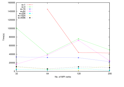
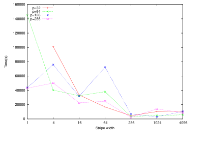
Figure 1: Left: Plot of the running time (in seconds, $y$-axis) of the sample Rheinfall implementation on the matrix M0,6-D10, versus the number $p$ of MPI ranks ($x$-axis). Right: Plot of the running time (in seconds, $y$-axis) of the sample Rheinfall implementation on the matrix M0,6-D10, versus stripe width $w$ ($x$-axis).

In order to assess the parallel performance and scalability of the sample “Rheinfall” implementation, the rank-computation program has been run on the matrix M0,6-D10 (from the Mgn group of SIMC [2]; see Table 1 for details). The program has been run with a varying number of MPI ranks and different values of the stripe width parameter $w$: see Figure 1.

The plots in Figure 1 show that running time generally decreases with higher $w$ and larger number $p$ of MPI ranks allocated to the computation, albeit not regularly. This is particularly evident in the plot of running time versus stripe width (Figure 1, right), which shows an alternation of performance increases and decreases. A more detailed investigation is needed to explain this behavior; we can only present here some working hypotheses.

The $w$ parameter influences communication in two different ways. On the one hand, there is a lower bound $O(m/w)$ on the time required to pass the End message from $P[0]$ to $P[m]$. Indeed, since the End message is always sent from one PU to the next one, then we only need to send one End message per stripe over the network. This could explain why running time is almost the same for $p=128$ and $p=256$ when $w=1$: it is dominated by the time taken to pass the End message along.

On the other hand, MPI messages are collected after each processing unit residing on a MPI rank has performed a round of elimination; this means that a single PU can slow down the entire MPI rank if it gets many elimination operations to perform. The percentage of running time spent executing MPI calls has been collected using the mpiP tool [8]; a selection of relevant data is available in Table 4. The three call sites for which data is presented measure three different aspects of communication and workload balance:

• The MPI_Recv figures measure the time spent in actual row data communication (the sending part uses MPI_Issend which returns immediately).

• The MPI_Iprobe calls are all done after all PUs have performed one round of elimination: thus they measure the time a given MPI rank has to wait for data to arrive.

• The MPI_Barrier is only entered after all PUs residing on a given MPI rank have finished their job; it is thus a measure of workload imbalance.

Now, processing units corresponding to higher column indices naturally have more work to do, since they get the rows at the end of the elimination chain, which have accumulated fill-in. Because of the way PUs are distributed to MPI ranks, a larger $w$ means that the last MPI rank gets more PUs of the final segment: the elimination work is thus more imbalanced. This is indeed reflected in the profile data of Table 4: one can see that the maximum time spent in the final MPI_Barrier increases with $w$ and the number $p$ of MPI ranks, and can even become 99% of the time for some ranks when $p=256$ and $w=4096$.

However, a larger $w$ speeds up delivery of Row messages from $P[c]$ to $P[c^{\prime}]$ iff $(c^{\prime}-c)/w\equiv 0(\textrm{mod\leavevmode\nobreak\ }p)$. Whether this is beneficial is highly dependent on the structure of the input matrix: internal regularities of the input data may result on elimination work being concentrated on the same MPI rank, thus slowing down the whole program. Indeed, the large percentages of time spent in MPI_Iprobe for some values of $p$ and $w$ show that the matrix nonzero pattern plays a big role in determining computation and communication in Rheinfall. Static analysis of the entry distribution could help determine an assignment of PUs to MPI ranks that keeps the work more balanced.

6 Conclusions and future work

The “Rheinfall” algorithm is basically a different way of arranging the operations of classical Gaussian Elimination, with a naturally parallel and distributed-memory formulation. It retains some important features from the sequential Gaussian Elimination; namely, it can be applied to general sparse matrices, and is independent of matrix entry type. Pivoting can be done in Rheinfall with strategies similar to those used for GEPP; however, Rheinfall is not equally suited for exact and inexact arithmetic.

Poor performance when compared to state-of-the-art algorithms and some inherent instability due to the dependency on detection of nonzero entries suggest that “Rheinfall” is not a convenient alternative for floating-point computations.

For exact arithmetic (e.g., integers), the situation is quite the opposite: up to our knowledge, “Rheinfall” is the first practical distributed-memory Gaussian Elimination algorithm capable of exact computations. In addition, it is competitive with existing implementations also when running sequentially.

The distributed-memory formulation of “Rheinfall” can easily be mapped on the MPI model for parallel computations. An issue arises on how to map Rheinfall’s Processing Units to actual MPI execution units; the simple column-cyclic distribution discussed in this paper was found experimentally to have poor workload balance. Since the workload distribution and the communication graph are both determined by the matrix nonzero pattern, a promising future direction could be to investigate the use of graph-based partitioning to determine the distribution of PUs to MPI ranks.

Matrix	rows	columns	nonzero	fill%	Rheinfall	LinBox
M0,6-D8	862290	1395840	8498160	0.0007	23.81	36180.55
M0,6-D10	616320	1274688	5201280	0.0007	23378.86	13879.62
olivermatrix.2	78661	737004	1494559	0.0026	2.68	115.76
Trec14	3159	15905	2872265	5.7166	116.86	136.56
GL7d24	21074	105054	593892	0.0268	95.42	61.14
IG5-18	47894	41550	1790490	0.0900	1322.63	45.95

Table 1: CPU times (in seconds) for computing the matrix rank of selected integer matrices; boldface font marks the best result in each row. The “Rheinfall” column reports times for the sample C++ implementation. The “LinBox” column reports times for the GEPP implementation in LinBox version 1.1.7. The programs were run on the UZH “Schroedinger” cluster, equipped with Intel Xeon X5560 CPUs @ 2.8GHz and running 64-bit SLES 11.1 Linux; codes were compiled with GCC 4.5.0 with options -O3 -march=native.

Matrix	Rheinfall (T)	Rheinfall	LinBox (T)	LinBox
M0,6-D8	No mem.	23.81	50479.54	36180.55
M0,6-D10	37.61	23378.86	26191.36	13879.62
olivermatrix.2	0.72	2.68	833.49	115.76
Trec14	No mem.	116.86	43.85	136.56
GL7d24	4.81	95.42	108.63	61.14
IG5-18	12303.41	1322.63	787.05	45.95

Table 2: CPU times (in seconds) for computing the matrix rank of selected integer matrices and their transposes; boldface font marks the best result in each row. The table compares running times of the Rheinfall/C++ and GEPP LinBox 1.1.7 codes. The columns marked with (T) report CPU times used for the transposed matrix. Computation of the transposes of matrices “M0,6-D8” and “Trec14” exceeded the available $24\,\mathrm{GB}$ of RAM. Hardware, compilation flags and running conditions are as in Table 1, which see also for matrix size and other characteristics.

Matrix	$N$	nonzero	fill%	Rheinfall	SuperLU
bbmat	38744	1771722	0.118	83.37	1756.84
g7jac200sc	59310	837936	0.023	87.69	1722.28
lhr71c	70304	1528092	0.030	No mem.	926.34
mark3jac140sc	64089	399735	0.009	92.67	1459.39
torso1	116158	8516500	0.063	97.01	1894.19
twotone	120750	1224224	0.008	91.62	1155.53

Table 3: Average Mflop/s attained in running LU factorization of square $N\times N$ matrices; boldface font marks the best result in each row. The table compares the performance of the sample Rheinfall/C++ LU factorization with SuperLU 4.2. The test matrices are a subset of those used in [5]. See Table 1 for hardware characteristics.

$p$	$w$	MPI Total%			MPI_Recv%		MPI_Iprobe%		MPI_Barrier%
		Avg.$\pm\sigma$	Max.	Min.	Avg.	Max.	Avg.	Max.	Avg.	Max.
16	16	$18.79\pm 0.32$	19.61	18.37	79.96	81.51	3.13	3.29	0.00	0.00
32	16	$11.54\pm 0.53$	12.87	10.93	4.41	71.97	14.19	14.97	0.00	0.00
64	16	$12.25\pm 0.20$	12.78	11.77	1.12	55.94	34.57	36.13	0.00	0.00
128	16	$20.51\pm 0.55$	23.87	19.33	31.62	35.06	61.08	64.17	0.00	0.00
16	256	$26.77\pm 1.79$	29.50	23.29	89.69	92.31	1.27	1.50	0.00	0.20
32	256	$10.17\pm 1.34$	13.57	7.83	78.51	85.33	13.10	18.08	0.00	0.01
64	256	$16.55\pm 2.16$	22.15	11.74	61.46	73.13	27.20	43.73	0.00	0.67
128	256	$15.43\pm 0.64$	18.65	14.35	6.15	10.97	90.98	95.27	0.00	0.02
256	256	$38.92\pm 1.94$	43.24	32.99	6.12	14.20	89.38	97.41	0.00	0.60
16	4096	$9.08\pm 1.62$	13.81	7.22	50.57	66.97	7.52	10.35	0.00	0.19
32	4096	$6.53\pm 1.97$	12.33	3.71	36.80	58.48	28.30	51.23	1.51	3.71
64	4096	$6.81\pm 1.52$	12.01	4.53	8.73	30.15	72.13	93.92	10.88	26.93
128	4096	$16.73\pm 7.80$	44.72	8.59	5.12	21.82	46.82	92.24	43.69	86.65
256	4096	$45.78\pm 28.32$	88.22	9.91	0.00	9.18	11.94	96.68	86.09	98.63

Table 4: Percentage of running time spent in MPI communication for the sample Rheinfall/C implementation on the matrix M0,6-D10, with varying number of MPI ranks and stripe width parameter $w$. Columns MPI_Recv, MPI_Iprobe and MPI_Barrier report on the percentage of MPI time spent spent servicing these calls; in these cases, the minimum is always very close to zero hence it is omitted from the table. Tests were executed on the UZH cluster “Schroedinger”; see Table 1 for hardware details. The MPI layer was provided by OpenMPI version 1.4.3, using the TCP/IP transport.

References

- [1] Dumas, J.G., Gautier, T., Giesbrecht, M., Giorgi, P., Hovinen, B., Kaltofen, E., Saunders, B.D., Turner, W.J., Villard, G.: LinBox: A Generic Library for Exact Linear Algebra. In: Cohen, A., Gao, X.S., Takayama, N. (eds.) Mathematical Software: ICMS 2002 (Proceedings of the first International Congress of Mathematical Software. pp. 40–50. World Scientific (2002)
- [2] Dumas, J.G.: The Sparse Integer Matrices Collection. http://ljk.imag.fr/membres/Jean-Guillaume.Dumas/simc.html
- [3] Dumas, J.G., Villard, G.: Computing the rank of large sparse matrices over finite fields. In: CASC’2002 Computer Algebra in Scientific Computing. pp. 22–27. Springer-Verlag (2002)
- [4] Golub, G., Van Loan, C.: Matrix Computation. Johns Hopkins University Press, 2nd edn. (1989)
- [5] Grigori, L., Demmel, J.W., Li, X.S.: Parallel symbolic factorization for sparse LU with static pivoting. SIAM J. Scientific Computing 29(3), 1289–1314 (2007)
- [6] LinBox website. http://linalg.org/
- [7] Valiant, L.G.: A bridging model for parallel computation. Commun. ACM 33, 103–111 (August 1990), http://doi.acm.org/10.1145/79173.79181
- [8] Vetter, J., Chambreau, C.: mpiP: Lightweight, Scalable MPI profiling. http://www.llnl.gov/CASC/mpiP (2004)