Quantum correlations and mutual synchronization

Abstract

We consider the phenomenon of mutual synchronization in a fundamental quantum system of two detuned quantum harmonic oscillators dissipating into the environment. We identify the conditions leading to this spontaneous phenomenon showing that the ability of the system to synchronize is related to the existence of disparate decay rates and is accompanied by robust quantum discord and mutual information between the oscillators, preventing the leak of information from the system.

I Introduction

Synchronization phenomena have been observed in a broad range of physical, chemical and biological systems under a variety of circumstances Pikovsky . In some instances, synchronization (also known as entrainment in this context) is induced by the presence of an external forcing or driving that acts as a pacemaker; in others it appears spontaneously as a consequence of the interaction between the elements. The latter case is the most relevant from the point of view of complexity since it appears as an emergent phenomenon that takes place despite the natural differences between the elements. Collective synchronization, whose simplest description can be given in terms of coupled self-sustained oscillators, is found in relaxation oscillator circuits, networks of neurons, cardiac pacemaker cells or fireflies that flash in unison Strogatz . A key ingredient for collective synchronization is dissipation, which is responsible for collapsing any trajectory of the system in phase space in a lower dimensional manifold.

Synchronization has also been studied in the quantum world in the case of entrainment induced by an external driving Hanggi . Difficulties in addressing quantum collective synchronization come from the fact that in linear oscillators dissipation will lead to the death of the oscillations after a transient while the extension to the quantum world of nonlinear phase oscillators does not allow for an insightful treatment. In this work, however, we take a step toward the understanding of quantum collective synchronization, showing that it is possible to fully characterize synchronization during the transient dynamics. We find that synchronization happens in the presence of a common bath due to a separation between dissipation rates. Different groups have recently approached this subject considering the (classical) synchronization of nanoscopic and microscopic systems susceptible of having quantum behavior Lipson ; Marquardt ; Milburn . In this work we establish the connections between the phenomenon of synchronization and quantum correlations in the system.

II System

We consider two coupled quantum harmonic oscillators dissipating into the environment PazRoncagliaPRLPRA ; Liugoan ; hupazang with different frequencies Galve_PRA2010 , which is arguably one of the most fundamental prototypical models. Current experimental realizations in the quantum regime include nanoelectromechanical structures and optomechanical devices NEMS_optomech as well as separately trapped ions whose direct coupling has been reported recently Wineland-Blatt . The system Hamiltonian for $\hbar=1$ and unit masses is

$$H_{S}=\frac{p_{1}^{2}}{2}+\frac{p_{2}^{2}}{2}+\frac{1}{2}(\omega_{1}^{2}x_{1}^{2}+\omega_{2}^{2}x_{2}^{2})+\lambda x_{1}x_{2},$$ (1)

where $|\lambda|<\omega_{1}\omega_{2}$ (attractive potential) and we allow for frequency diversity. The free Hamiltonian is diagonalized by a rotation in the $x_{1}-x_{2}$ plane, with $\theta$ the angle that gives the eigenvectors $\{{X}_{\pm}\}$ a function of the coupling $\tan 2\theta={2\lambda}/{\omega_{2}^{2}-\omega_{1}^{2}}$. Master equations for both a common bath (CB) and separate baths (SB) have been compared by also analyzing entanglement decay time in Ref. Galve_PRA2010 , where both the similarity of the frequencies of the oscillators and the coupling strength were shown to contribute to the preservation of entanglement for a CB, leading to asymptotic entanglement in the case of identical frequencies PazRoncagliaPRLPRA ; Prauzner ; Liugoan . The transition from SB to one CB underlies the capability of entanglement generation discussed in Ref. SB_CB and a physical implementation of the latter has been proposed recently Paz_CB .

Following Ref. Galve_PRA2010 , the system dynamics is described by a master equation that is valid in the weak-coupling limit between the system and environment, without the rotating-wave approximation breuer . Even if the obtained master equation has the same form as the exact one hupazang , the coefficients are approximated for weak coupling $\gamma$ between the system and environment. Taking this equation for strong coupling can lead to unphysical values for the reduced density and violation of positivity can appear at low temperatures and for certain initial states breuer . In the following we restrict our analysis to small $\gamma=0.01\omega_{1}$ where we never encounter any unphysical dynamics. This is consistent with the fact that deviations of this master equation from one in the Lindblad form (preserving positivity) are in fact small for high temperatures (here $T=10\omega_{1}$ in natural units). Particularly useful for the purpose of understanding the physical behavior of the oscillators dissipation is the master equation in the basis of the normal modes of the system Hamiltonian as given in Appendix A.

An important observation is that our results do not in fact depend on the specific choice of this master equation. In particular, in Appendix B we compare our results with the one obtained from a master equation in the Linblad form, obtained by a rotating-wave approximation. Within this approximation the master equation is known to be in the Lindblad form breuer ; rivas and we find almost exactly the same results as that obtained with the master equation (7). Therefore the phenomena predicted in the following do not depend on the specific details of the considered master equation.

III Synchronization

The dynamical behavior of the two oscillators can be analyzed through their average positions, variances, and correlations, as we deal here with Gaussian states. The presence of a CB or of two (even if identical) SB leads to different friction terms in the dynamical equations of both first- and second-order moments Galve_PRA2010 with profound consequences. We recall that for a CB only the sum of positions $x_{+}=x_{1}+x_{2}$ is actually dissipating and this does not coincide with $X_{+}$ unless the oscillators are identical.

Figure 1(a) shows the variance dynamics of two oscillators starting from two vacuum squeezed states. To quantify synchronization between two functions $f(t)$ and $g(t)$, we adopted a commonly used indicator, namely, $C_{f,g}(t,\Delta t)=\overline{\delta f\delta g}/\sqrt{\overline{\delta f^{2}}~{}\overline{\delta g^{2}}}$ where the bar stands for a time average $\overline{f}=\int_{t}^{t+\Delta t}dt^{\prime}f(t^{\prime})$ with time window $\Delta t$ and $\delta f=f-\overline{f}$. For similar evolutions $|C|\sim 1$, while $|C|\sim 0$ for different dynamics. The position variances for CB [Fig. 1(a)] show a transient dynamics without any similarity between them, also in antiphase ($C_{\langle x^{2}_{1}\rangle\langle x^{2}_{2}\rangle}<0$), before reaching full synchronization [Fig. 1(b)].

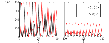
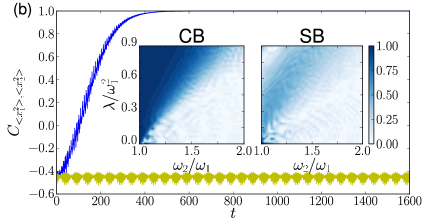
Figure 1: (a) $\langle x^{2}_{1}(t)\rangle/{\cal S}$ (light color) and $\langle x^{2}_{2}(t)\rangle/{\cal S}$ (black) normalized with the shot noise ${\cal S}$, for $\omega_{2}=1.4\omega_{1}$ and $\lambda=0.7\omega_{1}^{2}$ starting from squeezed states for a CB and (b) synchronization $C_{\langle x^{2}_{1}\rangle\langle x^{2}_{2}\rangle}(t,15)$ for a CB (dark color) and SB (light color) for temperature $T=10\omega_{1}$ (in natural units). The insets show synchronization values $|C_{\langle x^{2}_{1}\rangle\langle x^{2}_{2}\rangle}|$ varying $\omega_{2}/\omega_{1}$ and $\lambda/\omega_{1}^{2}$ at $t=300$. Time $t$ is scaled with $\omega_{1}$ (and is therefore adimensional) and $\gamma=0.01\omega_{1}$, here and in the following. The initial state is separable with squeezing parameters $2$ and $4$, respectively, in the two oscillators.

A comprehensive analysis shows that this behavior is robust considering (i) different initial conditions, (ii) any second-order moments of the two oscillators (either of positions $x_{1,2}$ or momenta $p_{1,2}$ or any arbitrary quadrature), and (iii) a whole range of couplings and detunings. Regarding (i), an important observation is that while in an isolated system the dynamics is strongly determined by the initial conditions, this is not the case in the presence of an environment. After a transient (in which the initial conditions have an important role), we actually find synchronization independently of the initial state, with detuning and oscillator coupling therefore being the only relevant parameters. The full analysis (iii) for a CB allows us to conclude that synchronization arises faster for nearly resonant oscillators and that the deteriorating effect of detuning can be proportionally compensated for by strong coupling, as represented in the CB inset of Fig. 1(b).

Moving now to the case of separate baths, a completely different scenario appears. The quality of the synchronization is generally poor (small $|C|$), not improving in time and dependent on the initial condition. The full parameters map for $|C|$ is shown in the SB inset of Fig. 1(b). In this case the oscillators do not synchronize in spite of their coupling even considering long times when finally the system thermalizes.

The appearance of a synchronous dynamics only for a CB can be understood by considering the time evolution of the second-order moments. The matrix governing their time evolution Galve_PRA2010 (see also Appendix A) has complex eigenvalues $\{\mu_{i}\}$ ($i=1,..,10$), named in the following dynamical eigenvalues. Their real and imaginary parts determine the decays and oscillatory dynamics of all second-order moments and variances. As shown in Fig. 2(a), when $\lambda=0$ all the eigenvalues are along the line $-0.01$ and for increasing coupling in the case of one CB they move in the complex plane assuming three different real values. In contrast, for SB all dynamical eigenvalues have similar real parts that remain almost unchanged when varying parameters. Hence for SB the ratio between the maximum and the minimum eigenvalues ${\rm Re}(\mu_{M})/{\rm Re}(\mu_{m})\approx 1$ is almost constant for all parameters, while for a CB $and$ for parameters for which synchronization is found [CB inset in Fig. 1(b)] ${\rm Re}(\mu_{M})/{\rm Re}(\mu_{m})<<1$, as shown in Fig. 2(b). In this parameters regime, after a transient time, only the least-damped eigenvector survives, thus fixing the frequency of the whole dynamics of the moments. As a consequence of this mechanism, synchronization is observed by considering the expectation values of any quadrature of the oscillators as well as higher-order moments.

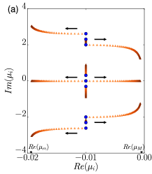
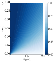
Figure 2: (a) Eigenvalues $\mu_{i}$ in the complex plane for a CB for $\omega_{2}/\omega_{1}=1.31$ and increasing the coupling from $\lambda=0$ [circles with ${\rm Re}(\mu_{i})\sim-0.01$] to $\lambda=0.9\omega_{1}^{2}$ in the direction of darker colors. (b) Ratio between minimum and maximum eigenvalue ${\rm Re}(\mu_{m})/{\rm Re}(\mu_{M})$ for a CB.

We obtain an approximated analytical estimation of time scales by considering the master equation in the eigenbasis $\{{X}_{\pm},{P}_{\pm}\}$ of the free Hamiltonian [Eq. (1], as detailed in Appendix A. The master equations for common and separate baths have the same expression in the case of detuned oscillators and the nature of dissipation (a CB or SB) appears only in the form of the damping coefficients. By eliminating the oscillating terms in the dynamics in the interaction picture, one obtains that, within this approximation, the decay rates of $\left<{P}_{\pm}^{2}\right>$ are given by

$$\tilde{\Gamma}_{\pm\pm}^{SB} = c^{2}\Gamma_{11}+s^{2}\Gamma_{22}\pm cs\Gamma_{12}$$ (2)

for SB and

$$\tilde{\Gamma}_{\pm\pm}^{CB}=(c\pm s)(c\Gamma_{11}\pm s\Gamma_{22})+(1\pm 2sc)\Gamma_{12}$$ (3)

for a CB, where $c=\cos\theta$, $s=\sin\theta$ (with $\theta$ previously defined diagonalization angle of $H_{S}$), and $\Gamma_{11,22,12}$ appear in the original master equation (see the Appendix of Ref. Galve_PRA2010 ). These approximated decays for the variances, together with their average $(\tilde{\Gamma}_{--}+\tilde{\Gamma}_{++})/2$ (for $\left<{P}_{+}{P}_{-}\right>$), for a CB and SB do agree very well with the real parts of the dynamical eigenvalues.

As mentioned before, synchronization (for a CB) is observed by looking at the dynamics of both first- and second-order moments: the ratio between minimum and maximum dynamical eigenvalues is the same in both cases. Still, our interest is in the second-order moments due to their relevance in the quantum information shared by the oscillators. Furthermore, inspection of first-order moment dynamics allows us to establish connections with what is known in classical systems Pikovsky . Two studied scenarios for classical synchronization are the diffusive coupling where both oscillator dampings depend on the difference of the velocity and the direct coupling where each one depends on the velocity of the other Pikovsky . The quantum harmonic oscillators considered here for a CB display in their first-order moments a diffusive coupling up to a change of sign, which explains the antiphase character of their synchronization.

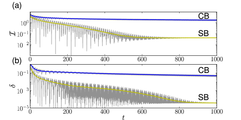
Figure 3: (a) Mutual information and (b) discord on a logarithmic scale for a common bath and separate baths (SB). Both the exact time evolutions and the filtered ones (Gaussian filter) are shown. The parameters are $\omega_{2}=1.05\omega_{1}$ and $\lambda=0.3\omega_{1}^{2}$.

IV Quantum correlations

Once the conditions for synchronization to arise have been established, we explore this phenomenon by focusing on the information aspects, through mutual information shared by the oscillators and their quantum correlations. In particular, the total correlations between the oscillators are measured by the mutual information ${\cal{I}}(\varrho)=S(\varrho_{1})+S(\varrho_{2})-S(\varrho)$ where $S$ stands for the von Neumann entropy, and $\varrho_{1(2)}$ is the reduced density matrix of each harmonic oscillator. A possible partition of correlations into quantum and classical parts that has received much attention recently is given by the quantum discord zurek ; vedral $\delta(\varrho)=\min_{\{\Pi_{i}\}}\left[S(\varrho_{2})-S(\varrho)+S(\varrho_{1}|\{\Pi_{i}\})\right]$, with the conditional entropy defined as $S(\varrho_{1}|\{\Pi_{j}\})=\sum_{i}p_{i}S(\varrho_{1|\Pi_{i}})$, $\varrho_{1|\Pi_{i}}=\Pi_{i}\varrho\Pi_{i}/{p_{i}}$ density matrix after a complete measurement $\{\Pi_{j}\}$ on the second oscillator, and $p_{i}={\rm Tr}_{12}(\Pi_{i}\varrho)$. The importance of this measure of the quantumness of correlations relies on its capability to distinguish and understand classical and quantum behaviors discord . Quantum discord has been reported recently also for continuous variables in Gaussian states paris-adesso .

Dissipation degrades all quantum and classical correlations ijqi . Nevertheless, important differences are found when comparing a CB and SB for the same parameter choices. In Fig. 3 we show a fast decay of all the total [Fig. 3(a)] and quantum [Fig. 3(b)] correlations for SB. In contrast, for a CB we find that after a short transient both mutual information and discord oscillate around an almost constant value and their decay is nearly frozen. For these parameters and a common environment the oscillators synchronize and $C_{\langle x^{2}_{1}\rangle\langle x^{2}_{2}\rangle}=0.95$ at $t\sim 270$. The robustness of the quantum correlations for long times in synchronizing oscillators in a CB and the deep differences with the case of SB is surprising also because their respective asymptotic values are really similar for detuned oscillators. In other words, the upper CB curve in Fig. 3(a) [or Fig. 3(b)] will eventually thermalize, converging to a value very similar the one obtained for SB, while strong differences in the asymptotic values actually appear only in the case of identical oscillators PazRoncagliaPRLPRA . As a further result, the effect of increasing the temperature is mostly on the asymptotic state while the main features of the dynamics described here are still observed.

We now focus on the case of a CB to look for specific quantum features of the synchronization exploring different parameters regimes. The comparison of mutual information and discord in cases in which there is synchronization or the system dissipates without having time to synchronize is given in Fig. 4 (upper and lower curves, respectively) where we filter out the fast oscillations to highlight the decay dynamics. For small coupling and large detuning, discord (shown in Fig. 4 for $\lambda/\omega_{1}^{2}=0.3$ and $\omega_{2}/\omega_{1}=1.4$) and mutual information are rapidly degraded. In this case, when $t=200$ there is no synchronous dynamics and $C_{\langle x^{2}_{1}\rangle\langle x^{2}_{2}\rangle}\sim 0$. In contrast, for strong coupling or for small detuning, synchronization occurs fast: for $\lambda/\omega_{1}^{2}=0.8$ and $\omega_{2}/\omega_{1}=1.05$, $C_{\langle x^{2}_{1}\rangle\langle x^{2}_{2}\rangle}(t=200)\sim 1$. In this case, after a short transient, the dynamics of discord is almost frozen and it remains $robust$ against decoherence. In exploring different parameter regimes we conclude that fast decay of classical and quantum correlations is found in cases in which there is no synchronization while the emergence of synchronization accompanies robust correlations against dissipation (frozen decay). The inset in Fig. 4 represents the value of the discord after the fast decay (here for $t=300$), where it is expected to be already in the plateau. There is a rather suggestive similarity to the synchronization map for a CB shown in the inset of Fig. 1(b). Considering that also entropy shows in this regime a slow growth, we conclude that synchronized oscillators are characterized by a reduced leakage of information into the environment.

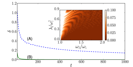
Figure 4: Evolution of the discord for a CB and the parameters $\omega_{2}/\omega_{1}=1.05$ and $\lambda=0.8\omega_{1}^{2}$ (dashed line A) and $\omega_{2}/\omega_{1}=1.4$ and $\lambda=0.3\omega_{1}^{2}$ (solid line B). The inset represents the quantum discord at $t=300$ for a CB.

One might wonder if the presence of a synchronous dynamics has any effect on entanglement, as in contrast with pure states mixed states with large quantum correlations can have even vanishing entanglement Galve_PRA2011 . The presence of the environment for oscillators with different frequencies leads to a complete loss of entanglement in finite short times unless the couplings to the CB are ”balanced” Galve_PRA2010 . In the general case of detuned oscillators, even for large couplings, entanglement decay is typically faster than the time scales at which the system reaches synchronous dynamics both for a CB and SB, mostly at this temperature ($T=10\omega_{1}$). Still, longer survival times for entanglement in a CB are found for small detunings and strong couplings Galve_PRA2010 .

V Dependence on initial conditions

We mentioned before that initial conditions do not play any important role in the appearance of synchronization. Indeed synchronous dynamics of the moments appears when an eigenmode dominates because of its slow dissipation rate and this goes beyond the specificity of the choice of the initial state. However, the details of the dynamics do depend on the latter as we illustrate for the following initial conditions:
(i) the separable vacuum state: $\rho=|0\rangle\langle 0|\otimes|0\rangle\langle 0|$
(ii) the two-mode squeezed states

$$\rho = U_{12}(r)\left(|0\rangle\langle 0|\otimes|0\rangle\langle 0|\right)U_{12}^{\dagger}(r)$$

where $U_{12}(r)=\exp{\left[-r(a_{1}^{\dagger}a_{2}^{\dagger}-a_{1}a_{2})/2\right]}$ and $a_{i}(a_{i}^{\dagger})$ are the usual annihilation (creation) operators; and (iii) the separable squeezed state:

$$\rho = U_{1}(r_{1})|0\rangle\langle 0|U_{1}^{\dagger}(r_{1})\otimes U_{2}(r_{2})|0\rangle\langle 0|U_{2}^{\dagger}(r_{2}),$$

with $U_{i}(r_{i})=\exp{\left[-r(a_{i}^{\dagger 2}-a_{i}^{2})/2\right]}$.

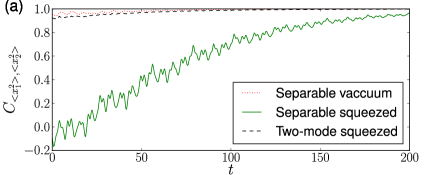
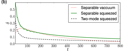
Figure 5: (a) Synchronization indicator and (b) decay of quantum correlations for different initial conditions in the case of a common bath: separable squeezed state with squeezings $r_{1}=2$ and $r_{2}=4$ (solid line), separable vacuum state (dotted line), and entangled two-mode squeezed state (dashed line) with squeezing $r=2$. Other parameters are $\omega_{2}/\omega_{1}=1.1$ and $\lambda=0.8\omega_{1}^{2}$

Instead, quantum correlations $\delta$ depend on the initial condition in the sense that more or less of the latter will be present. However after the short transient they always reach a plateau where information leakage to the environment is greatly reduced. Both information leakage reduction and synchronization are part of the same underlying phenomenon: that of a dissipation channel being much slower than the other. This behavior is seen in Fig. 5 where quantum correlations and the synchronization indicator are displayed for different initial conditions. We must further stress here that, since the asymptotic thermal state has $\delta\sim 10^{-4}$, the plateau is expected to be very long.

VI Conclusions

Our analysis of the dynamics of dissipative quantum harmonic oscillators has allowed us to establish under which conditions synchronization appears. This phenomenon can appear in rather different forms but, in this paper it was reported during the transient dynamics of a (quantum or classical) system coupled to an environment and relaxing toward equilibrium. The emergence of synchronization was explained in terms of different temporal decays governing the system evolution and related to a separation between the eigenvalues of the matrix generating the dynamics. We traced synchronization between second-order moment evolution from the existence of a slowly decaying eigenmode and found approximated expressions for the variance decay coefficients in very good agreement with the real parts of the dynamical eigenvalues. We found that synchronization arises in the presence of a common bath, but not for separate ones, for any strength of the coupling between oscillators. It could be of interest to study the transition between such different scenarios SB_CB . The relevant parameters are $\lambda/\omega_{1}^{2}$ and $\omega_{2}/\omega_{1}$ since the dependence on initial conditions is actually weak.

We have then characterized mutual synchronization from a quantum information perspective through mutual information and quantum discord exploring their dynamics in different parameters regimes. We found that there is a signature of synchronization in the information shared by the oscillators. We have shown that discord and mutual information are more robust when the oscillators synchronize. In spite of the fact that after thermalizing the asymptotic discord is negligible for both a CB and SB, the decay toward this value is clearly frozen in the presence of synchronization. In this case total and quantum correlations display a very slow decay (plateau) and the leak of information into the bath is reduced. The identification of the conditions for the occurrence of synchronization and its connection with quantum correlations reported here provides the path towards future extensions such as the study of arrays and networks, the analysis of the role of different environments, or the exploration of eventual connections with biological systems in which synchronization is a widespread phenomenon.

Appendix A Master equation in the normal modes basis

The master equations describing the evolution of the reduced density matrix of the system of two different oscillators, up to second order in the coupling strength, have been reported in Ref. Galve_PRA2010 for both a common and separate baths. Here we provide these equations in the basis of the eigenmodes of the Hamiltonian. We stress that the exact master equation at all coupling orders has the same structure as ours, the difference being in the form of its coefficients breuer ; hupazang . For weak coupling this equation is a very good approximation to the exact one. Furthermore, in Appendix B we show that the full evolution almost perfectly matches that of a master equation obtained by a rotating-wave approximation, the latter being always positive due to its Lindblad form.

A.1 Common bath

In the case of a common bath, we assume for the interaction Hamiltonian between the system and the environment the form $H_{I}^{CB}=\sum_{k}g_{k}(b_{k}+b_{k}^{\dagger})x_{+}$, where $x_{+}=x_{1}+x_{2}$, $b_{k}(b_{k}^{\dagger})$ creates (annihilates) an excitation (with energy $\Omega_{k}$) over the $k$th mode of the bath, and where the coupling coefficients $g_{k}$ are related to the density of states of the bath $J(\Omega)$ through $J(\Omega)=\sum_{k}\left(g_{k}^{2}/\Omega_{k}\right)\delta(\Omega-\Omega_{k})$. We assume an Ohmic environment with a Lorentz-Drude cut-off function, whose spectral density is

$$J(\Omega)=\frac{2\gamma}{\pi}\Omega\frac{\Lambda^{2}}{\Lambda^{2}+\Omega^{2}}.$$ (4)

The results represented in this work are obtained with bath-system coupling $\gamma=0.01\omega_{1}$ and cutoff $\Lambda=50\omega_{1}$.

The eigenvectors of $H_{S}$ are

$$X_{-} = \cos\theta x_{1}-\sin\theta x_{2},$$ (5)

$$X_{+} = \cos\theta x_{2}+\sin\theta x_{1},$$ (6)

with $\tan 2\theta={2\lambda}/{\omega_{2}^{2}-\omega_{1}^{2}}$. The system eigenfrequencies $\Omega_{\pm}$ are always different due to the coupling ${2}\Omega_{\pm}^{2}=\omega_{1}^{2}+\omega_{2}^{2}\pm\sqrt{4\lambda^{2}+(\omega_{2}^{2}-\omega_{1}^{2})^{2}}$. Neglecting energy renormalization, the master equation in this eigenvector basis reads

$$\frac{d\rho(t)}{dt}=-i[H_{S},{\rho}(t)]-\frac{\tilde{D}^{CB}_{--}}{2}[X_{-},[X_{-},\rho]]-\frac{\tilde{D}^{CB}_{++}}{2}[X_{+},[X_{+},\rho]]-\tilde{D}^{CB}_{+-}[X_{+},[X_{-},\rho]]$$

$$+\frac{\tilde{F}^{CB}_{--}}{2}[X_{-},[P_{-},\rho]]+\frac{\tilde{F}^{CB}_{++}}{2}[X_{+},[P_{+},\rho]]+\frac{\tilde{F}^{CB}_{+-}}{2}[X_{+},[P_{-},\rho]]+\frac{\tilde{F}^{CB}_{-+}}{2}[X_{-},[P_{+},\rho]]$$

$$-i\left(\frac{\tilde{\Gamma}^{CB}_{--}}{2}[X_{-},\{P_{-},\rho\}]+\frac{\tilde{\Gamma}^{CB}_{++}}{2}[X_{+},\{P_{+},\rho\}]+\frac{\tilde{\Gamma}^{CB}_{+-}}{2}[X_{+},\{P_{-},\rho\}]+\frac{\tilde{\Gamma}^{CB}_{-+}}{2}[X_{-},\{P_{+},\rho\}]\right),$$ (7)

with

$$\tilde{D}^{CB}_{--} = (c-s)(cD_{11}-sD_{22})+(1-2sc)D_{12}$$

$$\tilde{D}^{CB}_{++} = (c+s)(cD_{11}+sD_{22})+(1+2sc)D_{12}$$

$$\tilde{D}^{CB}_{+-} = \frac{c^{2}-s^{2}}{2}(D_{11}+D_{22}+2D_{12})+sc(D_{11}-D_{22})$$

$$\tilde{F}^{CB}_{--} = (c-s)(cF_{11}-sF_{22})+(1-2sc)F_{12}$$

$$\tilde{F}^{CB}_{++} = (c+s)(cF_{11}+sF_{22})+(1+2sc)F_{12}$$

$$\tilde{F}^{CB}_{-+} = (c-s)(cF_{22}+sF_{11})+(c^{2}-s^{2})F_{12}$$

$$\tilde{F}^{CB}_{+-} = (c+s)(cF_{11}-sF_{22})+(c^{2}-s^{2})F_{12}$$

$$\tilde{\Gamma}^{CB}_{--} = (c-s)(c\Gamma_{11}-s\Gamma_{22})+(1-2sc)\Gamma_{12}$$

$$\tilde{\Gamma}^{CB}_{++} = (c+s)(c\Gamma_{11}+s\Gamma_{22})+(1+2sc)\Gamma_{12}$$

$$\tilde{\Gamma}^{CB}_{-+} = (c-s)(c\Gamma_{22}+s\Gamma_{11})+(c^{2}-s^{2})\Gamma_{12}$$

$$\tilde{\Gamma}^{CB}_{+-} = (c+s)(c\Gamma_{11}-s\Gamma_{22})+(c^{2}-s^{2})\Gamma_{12}$$ (8)

where $c=\cos\theta$, $s=\sin\theta$, and the dissipation ($\Gamma_{i,j}$) and diffusion ($D_{i,j},F_{i,j}$) coefficients are defined in the Appendix of Ref. Galve_PRA2010 , specifically in Eqs. (A18)-(A20). The related set of equations of motion is

$$\frac{d\langle X_{i}X_{j}\rangle}{dt} = \frac{1}{2}\left(\{X_{i},P_{j}\}+\{X_{j},P_{i}\}\right)$$ (9)

$$\frac{d\langle P_{i}P_{j}\rangle}{dt} = -\frac{1}{2}(\Omega_{i}^{2}\langle\{X_{i},P_{j}\}\rangle+\Omega_{j}^{2}\langle\{X_{j},P_{i}\}\rangle)$$ (10)

$$- (\tilde{\Gamma}^{CB}_{i,i}+\tilde{\Gamma}^{CB}_{j,j})\langle P_{i}P_{j}\rangle-\tilde{\Gamma}^{CB}_{i,-i}\langle P_{j}P_{-i}\rangle$$

$$- \tilde{\Gamma}^{CB}_{j,-j}\langle P_{i}P_{-j}\rangle+\tilde{D}^{CB}_{i,j}$$

$$\frac{d\langle\{X_{i},P_{j}\}\rangle}{dt} = 2\langle P_{i}P_{j}\rangle-2\Omega_{j}^{2}\langle X_{i}X_{j}\rangle+\tilde{F}^{CB}_{i,j}$$ (11)

$$- \tilde{\Gamma}^{CB}_{j,j}\langle\{X_{i},P_{j}\}\rangle-\tilde{\Gamma}^{CB}_{j,-j}\langle X_{i}P_{-j}\rangle$$

where $i,j=+,-$.

The time evolution of the vector ${\bf{R}}$ of all ten moments can be written in a compact matrix form

$$\dot{\bf{R}}=\mathcal{M}{\bf{R}}+{\bf N}.$$ (12)

The complex eigenvalues of $\mathcal{M}$ are $\{\mu_{i}\}$ with $i=1...10$, elsewhere referred as dynamical eigenvalues.

A.2 Separate baths

When the two environments are thought to be identical and independent from each other, the interaction Hamiltonian becomes

$$H_{I}^{SB}=\sum_{i=1}^{2}\sum_{k}g_{k}(b_{k}^{i}+b_{k}^{i\dagger})x_{i}$$ (13)

where the annihilation (creation) operators $b_{k}^{i}(b_{k}^{i\dagger})$ belong, respectively, to the $i$th thermal bath. The density of states of both of them is that of Eq. (4), with the same $\gamma$ and $\Lambda$ introduced before. The master equation has the same structure of Eq. (7) but the coefficients are modified as follows:

$$\tilde{D}^{SB}_{--} = c^{2}D_{11}+s^{2}D_{22}-2csD_{12}$$

$$\tilde{D}^{SB}_{++} = c^{2}D_{11}+s^{2}D_{22}+2csD_{12}$$

$$\tilde{D}^{SB}_{+-} = cs(D_{11}-D_{22})+(c^{2}-s^{2})D_{12}$$

$$\tilde{F}^{SB}_{--} = c^{2}F_{11}+s^{2}F_{22}-2csF_{12}$$

$$\tilde{F}^{SB}_{++} = c^{2}F_{11}+s^{2}F_{22}+2csF_{12}$$

$$\tilde{F}^{SB}_{-+} = \tilde{F}^{SB}_{+-}=cs(F_{11}-F_{22})+(c^{2}-s^{2})F_{12}$$

$$\tilde{\Gamma}^{SB}_{--} = c^{2}\Gamma_{11}+s^{2}\Gamma_{22}-2cs\Gamma_{12}$$

$$\tilde{\Gamma}^{SB}_{++} = c^{2}\Gamma_{11}+s^{2}\Gamma_{22}+2cs\Gamma_{12}$$

$$\tilde{\Gamma}^{SB}_{-+} = \tilde{\Gamma}^{SB}_{+-}=cs(\Gamma_{11}-\Gamma_{22})+(c^{2}-s^{2})\Gamma_{12}$$ (14)

Once these coefficients are used instead of those coming from a common bath, the equations of motion are formally identical to those of Eqs. (9)-(11).

Appendix B Independent decay rates

The eigenmodes (5) and (6) diagonalize the Hamiltonian of the system $H_{S}$ but are still indirectly coupled through the heat bath(s) as seen from Eqs. (9)-(11). This means that the eigenmodes cannot be considered as independent channels for dissipation. Yet if we rewrite their master equation in interaction picture, we can neglect fast oscillating terms, as usual in the rotating-wave approximation, that is, eliminate exponents such as $e^{\pm i(\Omega_{+}+\Omega_{-})t}$ due to their highly oscillatory behavior in comparison with the overall slower dynamics rivas ; vasile . If we takethatwhich also rotate though more slowly, those such as $e^{\pm i(\Omega_{+}-\Omega_{-})t}$, and keep only nonrotating terms. Finally, this procedure leads to an effective total decoupling of the eigenmodes, which then dissipate independently to the heat bath(s) with the decay rates $\tilde{\Gamma}_{\pm\pm}^{CB}$ and $\tilde{\Gamma}_{\pm\pm}^{SB}$ [Eqs. (2) and (3)]. In some sense this time averaging approximation can be seen as renormalizing all dissipation coefficients having mixed indices $+-$ (and $-+$) to zero, hence rendering the master equation as a tensor product of two independent evolutions. This could seem a bit too far fetched, but a comparison of the full dynamics and this approximation seems to be quite accurate as clear from Fig. 6, where we compare $\tilde{\Gamma}_{\pm\pm}^{CB}$ and their average with the three different values of ${\rm Re}(\mu_{i})$.

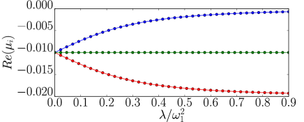
Figure 6: Rates $\tilde{\Gamma}_{++}^{CB}$, $\tilde{\Gamma}_{--}^{CB}$, from Eq. (3) and and $(\tilde{\Gamma}_{++}^{CB}+\tilde{\Gamma}_{--}^{CB})/2$ (dots) are compared with the (three different) real parts of the dynamical eigenvalues ${\rm Re}(\mu_{i})$ (continuous line) in the case of a common bath for $\omega_{2}/\omega_{1}=1.31$.

Inspection of these analytical expressions when varying system parameters confirms that dynamical eigenmode decays for SB all have similar real parts (in general $\Gamma_{12}$ small and $\Gamma_{11}\simeq\Gamma_{22}$), while for a CB the decays can be significantly different (a factor $20$ in Fig. 6). This difference between decay rates can be up to several orders of magnitude for parameters where synchronization appears faster. Synchronization is therefore linked to imbalanced dissipation rates of the eigenmodes, allowing the mode that survives longer to govern the dynamics. Within the discussed approximation its frequency is found to be $2\Omega_{-}$ with $\Omega_{-}$ previously defined as the frequency of the eigenmode $X_{-}$. This is independent of bath coefficients and we find very good agreement with the exact frequency.

It can be easily seen that the rotating-wave approximation described in this appendix, neglecting all highly oscillatory terms with exponents $e^{\pm i(\Omega_{+}\pm\Omega_{-})t}$, leads to (CB and SB) master equations in the Kossakowski-Lindblad form breuer . In particular, in the case of a common bath it can be found that

$$\frac{d\rho}{dt} = -i[H_{S},{\rho}(t)]$$

$$- \sum_{i=+,-}\frac{(\tilde{D}^{CB}_{ii}/\Omega_{i})+\tilde{\Gamma}^{CB}_{ii}}{4}[A_{i}^{\dagger}A_{i}\rho+\rho A_{i}^{\dagger}A_{i}-2A_{i}\rho A_{i}^{\dagger}]$$

$$- \sum_{i=+,-}\frac{(\tilde{D}^{CB}_{ii}/\Omega_{i})-\tilde{\Gamma}^{CB}_{ii}}{4}[A_{i}A_{i}^{\dagger}\rho+\rho A_{i}A_{i}^{\dagger}-2A_{i}^{\dagger}\rho A_{i}]$$

where $A_{\pm}=\sqrt{\Omega_{\pm}/2}X_{\pm}+i/\sqrt{2\Omega_{\pm}}P_{\pm}$. In spite of formal differences between Eqs. (7) and (B) we actually find very good agreement between their dynamical evolutions. In Fig. 7 we show that, in the limit of weak coupling considered here, predictions for synchronization and discord are actually almost indistinguishable. Maximum deviations in this case are at least two order of magnitude smaller than the represented quantities. As expected, deviations increase for stronger system-environment coupling. The really weak dependence on the details of the master equation [Eqs. (7) and (B)] when comparing the dynamical behavior of synchronization and quantum correlations between the oscillators further strengthens the generality of our results.

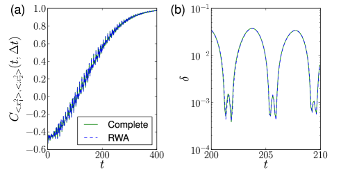
Figure 7: (a) Synchronization and (b) discord obtained from the complete master equation (7) compared with the values obtained after the rotating-wave approximation as described in the text in the case of common bath for $\omega_{2}/\omega_{1}=1.4,~{}\lambda=0.7\omega_{1}^{2}$.

References

- (1) A. Pikovsky, M. Rosenblum, J. Kurths, Synchronization: A Universal Concept in Nonlinear Sciences (Cambridge University Press, Cambridge, 2001).
- (2) S.H. Strogatz, Nonlinear Dynamics And Chaos: With Applications To Physics, Biology, Chemistry, And Engineering, (Westview, BOulder, CO, 2001).
- (3) I. Goychuk, J. Casado-Pascual, M. Morillo, J. Lehmann, and P. Hänggi, Phys. Rev. Lett. 97, 210601 (2006); O. V. Zhirov and D. L. Shepelyansky, ibid. 100, 014101 (2008); S-B. Shim, M. Imboden and P. Mohanty, Science, 316, 95 (2007).
- (4) M.Zhang, G. Wiederhecker, S. Manipatruni, A. Barnard, P. L. McEuen and M. Lipson, arXiv:1112.3636v1.
- (5) G. Heinrich, M. Ludwig, J. Qian, B. Kubala and F. Marquardt, Phys. Rev. Lett. 107 043603 (2011).
- (6) C. A. Holmes, C. P. Meaney, G. J. Milburn, arXiv:1105.2086.
- (7) J. P. Paz and A. J. Roncaglia, Phys. Rev. Lett. 100, 220401 (2008); J. P. Paz and A. J. Roncaglia, Phys. Rev. A 79, 032102 (2009).
- (8) K-L. Liu and H-S. Goan, Phys. Rev. A 76 022312 (2007)
- (9) B. L. Hu, J. P. Paz and Y. Zhang, Phys. Rev. D 45 2843 (1992); C-H. Chou, T. Yu, B. L. Hu, Phys. Rev. E 77 011112 (2008)
- (10) F. Galve, G. L. Giorgi and R. Zambrini, Phys. Rev. A 81, 062117 (2010).
- (11) T. Rocheleau, T. Ndukum, C. Macklin, J. B. Hertzberg, A. A. Clerk, and K. C. Schwab, Nature (London) 463, 72 (2010); D. Van Thourhout and J. Roels, Nature Phot. 4 211, (2010); F. Marino, F. S. Cataliotti, A. Farsi, M. Siciliani de Cumis, and Francesco Marin, Phys. Rev. Lett. 104, 073601 (2010); P. Verlot, A. Tavernarakis, T. Briant, P.-F. Cohadon, and A. Heidmann, Phys. Rev. Lett. 104, 133602 (2010);
- (12) K. R. Brown, C. Ospelkaus, Y. Colombe, A. C. Wilson, D. Leibfried, and D. J. Wineland, Nature (London), 471, 196 (2011); M. Harlander, R. Lechner, M. Brownnutt, R. Blatt, and W. Hänsel,ibid. 471, 200 (2011).
- (13) J. S. Prauzner-Bechcicki, J. Phys. A: Math. Gen., 37 L173 (2004)
- (14) T. Zell, F. Queisser, and R. Klesse , Phys. Rev. Lett. 102, 160501 (2009).
- (15) C. Cormick and J. P. Paz, Phys. Rev. A 81, 022306 (2010)
- (16) H. P. Breuer and F. Petruccione The Theory of Open Quantum Systems (2002, Oxford University Press).
- (17) A. Rivas, A. D. K. Plato, S. F. Huelga and M. B. Plenio, New J. Phys. 12, 113032 (2010)
- (18) H. Ollivier and W. H. Zurek, Phys. Rev. Lett. 88, 017901 (2001).
- (19) L. Henderson and V. Vedral, J. Phys. A 34, 6899 (2001).
- (20) A. Datta, A. Shaji, and C. M. Caves, Phys. Rev. Lett. 100, 050502 (2008); B. P. Lanyon, M. Barbieri, M. P. Almeida and A. G. White, ibid. 101, 200501 (2008); L. Mazzola, J. Piilo, and S. Maniscalco, ibid. 104, 200401 (2010); T. Werlang, C. Trippe, G. A. P. Ribeiro and G. Rigolin, ibid. 105, 095702 (2010).
- (21) P. Giorda and M. G. A. Paris, Phys. Rev. Lett. 105, 020503 (2010); G. Adesso and A. Datta, ibid. 105, 030501 (2010).
- (22) G. L. Giorgi, F. Galve, and R. Zambrini, Int. J. Quantum Inf. 9, 1825 (2011).
- (23) F. Galve, G. L. Giorgi, and R. Zambrini, Phys. Rev. A 83, 012102 (2011).
- (24) R. Vasile, S. Olivares, M. G. A. Paris, and S. Maniscalco, Phys. Rev. A 80 062324 (2009).