Functional A Posteriori Error Estimates for Elliptic Problems in Exterior Domains

Abstract

This paper is concerned with the derivation of computable and guaranteed upper bounds of the difference between the exact and the approximate solution of an exterior domain boundary value problem for a linear elliptic equation. Our analysis is based upon purely functional argumentation and does not attract specific properties of an approximation method. Therefore, the estimates derived in the paper at hand are applicable to any approximate solution that belongs to the corresponding energy space. Such estimates (also called error majorants of the functional type) have been derived earlier for problems in bounded domains of $\mathbb{R}^{N}$ (see [2, 3]).
Key Words A posteriori error estimates of functional type, elliptic boundary value problems in exterior domains
AMS MSC-Classifications 65 N 15

1 Introduction

The main focus of our investigations is to suggest a method of deriving guaranteed and computable upper bounds of the difference between the exact solution $u$ of an elliptic exterior domain boundary value problem and any approximation from the corresponding energy space. We discuss the method with the paradigm of the prototypical elliptic problem

$$-\operatorname{div}A\nabla u =f \text{in }\Omega,\makebox[0.0pt]{}$$ (1.1)

$$u|_{\gamma} =g \text{on }\gamma:=\operatorname{\partial}\Omega.\makebox[0.0pt]{}$$ (1.2)

We assume that $\Omega\subset\mathbb{R}^{N}$ with $N\geq 1$ is an exterior domain, i.e. $\mathbb{R}^{N}\setminus\Omega$ is compact, with Lipschitz continuous boundary $\gamma$ (see Figure 1).

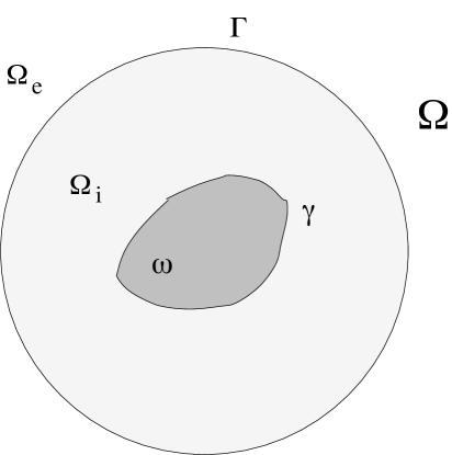
Figure 1: exterior domain $\Omega$ with artificial interface $\Gamma$

Throughout this paper we will use the weighted Lebesgue function spaces

$$\operatorname{\mathsf{L}}^{2}_{s}(\Omega):=\left\{\varphi\,\mid\,\rho^{s}\varphi\in\operatorname{\mathsf{L}}^{2}(\Omega)\right\},\quad s\in\mathbb{R}.$$

Here $\rho:=(1+r^{2})^{1/2}$ and $r(x):=|x|$ denotes the radius vector. $\operatorname{\mathsf{L}}^{2}_{s}(\Omega)$ is a Hilbert space equipped with the scalar product

$$\left\langle\varphi,\psi\right\rangle_{s,\Omega}:=\left\langle\rho^{s}\varphi,\rho^{s}\psi\right\rangle_{\Omega}:=\int_{\Omega}\rho^{2s}\varphi\psi\,\text{d}\lambda,$$

where $\varphi$ and $\psi$ belong to $\operatorname{\mathsf{L}}^{2}_{s}(\Omega)$ and $\lambda$ is Lebesgue’s measure. We denote the corresponding norms by $\left|\left|\varphi\right|\right|_{s,\Omega}=\left|\left|\rho^{s}\varphi\right|\right|_{\Omega}$. If $s=0$ then $\operatorname{\mathsf{L}}^{2}_{s}(\Omega)$ coincides with the usual Lebesgue space $\operatorname{\mathsf{L}}^{2}(\Omega)$. For the sake of simplicity we keep the same notation for spaces of vector-valued functions. Moreover, we introduce the weighted Sobolev space

$$\overset{}{\operatorname{\mathsf{H}}}{}^{1}_{-1}(\Omega):=\left\{\varphi\in\operatorname{\mathsf{L}}^{2}_{-1}(\Omega)\,\mid\,\nabla\varphi\in\operatorname{\mathsf{L}}^{2}(\Omega)\right\},$$

which is a Hilbert space as well with respect to the scalar product

$$(\varphi,\psi)\mapsto\left\langle\varphi,\psi\right\rangle_{-1,\Omega}+\left\langle\nabla\varphi,\nabla\psi\right\rangle_{\Omega}.$$

By $\overset{\circ}{\operatorname{\mathsf{H}}}{}^{1}_{-1}(\Omega)$ we denote the closure of $\overset{\circ}{\operatorname{\mathsf{C}}}{}^{\infty}(\Omega)$, the space of compactly supported smooth test functions, in the norm of $\overset{}{\operatorname{\mathsf{H}}}{}^{1}_{-1}(\Omega)$. Whenever we consider Sobolev spaces of bounded domains we use the usual unweighted $\operatorname{\mathsf{L}}^{2}$-scalar products and -norms.

For dimensions $N\geq 3$ the solution theory for the problem (1.1)-(1.2) is based on the weighted Poincare/Friedrich estimate (see Corollary 16 (i) and Remark 17 of the appendix)

$$\left|\left|\varphi\right|\right|_{-1,\Omega}\leq\frac{2}{N-2}\left|\left|\nabla\varphi\right|\right|_{\Omega}\quad\forall\,\varphi\in\overset{\circ}{\operatorname{\mathsf{H}}}{}^{1}_{-1}(\Omega),\makebox[0.0pt]{}$$ (1.3)

the Lax-Milgram theorem and, if needed, an adequate extension operator for the boundary data. Let $u_{\gamma}$ be some function in $\overset{}{\operatorname{\mathsf{H}}}{}^{1}_{-1}(\Omega)$ satisfying the boundary condition (1.2). The weak solution $u\in\overset{\circ}{\operatorname{\mathsf{H}}}{}^{1}_{-1}(\Omega)+u_{\gamma}\subset\overset{}{\operatorname{\mathsf{H}}}{}^{1}_{-1}(\Omega)$ of (1.1)-(1.2) is then defined by the variational formulation

$$\left\langle A\nabla u,\nabla w\right\rangle_{\Omega} =\left\langle f,w\right\rangle_{\Omega}\quad\forall\,w\in\overset{\circ}{\operatorname{\mathsf{H}}}{}^{1}_{-1}(\Omega).\makebox[0.0pt]{}$$ (1.4)

By (1.3) the left hand side of (1.4) is a strongly coercitive sesqui-linear form over $\overset{\circ}{\operatorname{\mathsf{H}}}{}^{1}_{-1}(\Omega)$ provided that the real-matrix-valued function $A$ is measurable, bounded a.e., symmetric and uniformly strongly elliptic, i.e.

$$\exists\,c_{A}>0\quad\forall\,\xi\in\mathbb{R}^{N}\quad\forall\,x\in\Omega\quad c_{A}|\xi|^{2}\leq A(x)\xi\cdot\xi.\makebox[0.0pt]{}$$ (1.5)

If $f\in\operatorname{\mathsf{L}}^{2}_{1}(\Omega)$ then by the Cauchy-Scharz inequality the right hand side of (1.4) is a linear and continuous functional over $\overset{\circ}{\operatorname{\mathsf{H}}}{}^{1}_{-1}(\Omega)$. Thus, under these assumptions the problem (1.4) is uniquely solvable in $\overset{\circ}{\operatorname{\mathsf{H}}}{}^{1}_{-1}(\Omega)+u_{\gamma}$ by Lax-Milgram’s theorem.

If $N=1,2$ one can apply the same arguments with the difference that (1.3) has to be modified. For $N=1$ and, for example, $\Omega\subset\mathbb{R}_{+}$ we have by Corollary 16 (iii) and Remark 17

$$\left|\left|\varphi\right|\right|_{-1,\Omega}\leq 2\left|\left|\varphi^{\prime}\right|\right|_{\Omega}\quad\forall\,\varphi\in\overset{\circ}{\operatorname{\mathsf{H}}}{}^{1}_{-1}(\Omega).\makebox[0.0pt]{}$$ (1.6)

Hence, we get the same solution theory with tiny restrictions on $\Omega$, which easily can be removed by a translation. For $N=2$ the singularities are stronger and additionally we have to utilize logarithmic terms. By Corollary 16 (ii) and Remark 17 we have for domains $\Omega\subset\mathbb{R}^{2}$, such that the complement $\mathbb{R}^{2}\setminus\Omega$ contains the unit ball,

$$\left|\left|\varphi/(r\ln r)\right|\right|_{\Omega}\leq 2\left|\left|\nabla\varphi\right|\right|_{\Omega}\quad\forall\,\varphi\in\overset{\circ}{\operatorname{\mathsf{H}}}{}^{1}_{-1,\ln}(\Omega),\makebox[0.0pt]{}$$ (1.7)

where

$$\overset{}{\operatorname{\mathsf{H}}}{}^{1}_{-1,\ln}(\Omega):=\left\{\varphi\,\mid\,\varphi/(r\ln r),\nabla\varphi\in\operatorname{\mathsf{L}}^{2}(\Omega)\right\}$$

is a Hilbert space equipped with the natural scalar product

$$(\varphi,\psi)\mapsto\left\langle\varphi/(r\ln r),\psi/(r\ln r)\right\rangle_{\Omega}+\left\langle\nabla\varphi,\nabla\psi\right\rangle_{\Omega}$$

and again $\overset{\circ}{\operatorname{\mathsf{H}}}{}^{1}_{-1,\ln}(\Omega)$ denotes the closure of $\overset{\circ}{\operatorname{\mathsf{C}}}{}^{\infty}(\Omega)$ in the norm of $\overset{}{\operatorname{\mathsf{H}}}{}^{1}_{-1,\ln}(\Omega)$. Consequently, we obtain for all $f$ with $r\ln rf\in\operatorname{\mathsf{L}}^{2}(\Omega)$ and all $u_{\gamma}$ in $\overset{}{\operatorname{\mathsf{H}}}{}^{1}_{-1,\ln}(\Omega)$ satisfying the boundary condition (1.2) a unique solution $u$ belonging to $\overset{\circ}{\operatorname{\mathsf{H}}}{}^{1}_{-1,\ln}(\Omega)+u_{\gamma}$.

We summarize the results in the following

Theorem 1

Let $N\geq 3$ as well as $f\in\operatorname{\mathsf{L}}^{2}_{1}(\Omega)$ and $u_{\gamma}\in\overset{}{\operatorname{\mathsf{H}}}{}^{1}_{-1}(\Omega)$ satisfying the boundary condition (1.2). Then the exterior boundary value problem (1.1)-(1.2) is uniquely weakly solvable in $\overset{\circ}{\operatorname{\mathsf{H}}}{}^{1}_{-1}(\Omega)+u_{\gamma}$. The solution operator is continuous.

From the above discussion, it is clear that for $N=1,2$ the existence of weak solutions in suitable spaces can also be proved.

Remark 2

The boundary data $g$ and its extension $u_{\gamma}$ can be described in more detail. In the bounded domain case it is well known that there exists a bounded linear trace operator and a corresponding bounded linear extension operator (right inverse) mapping $\overset{}{\operatorname{\mathsf{H}}}{}^{1}(\Omega)$ to $\overset{}{\operatorname{\mathsf{H}}}{}^{1/2}(\gamma)$ and vice verse. Hence, by restriction we get a bounded linear trace operator

$$\tau_{\gamma}:\overset{}{\operatorname{\mathsf{H}}}{}^{1}_{-1}(\Omega)\to\overset{}{\operatorname{\mathsf{H}}}{}^{1/2}(\gamma)$$

and by extension and applying an obvious cutting technique we obtain a bounded linear extension operator

$$E:\overset{}{\operatorname{\mathsf{H}}}{}^{1/2}(\gamma)\to\overset{}{\operatorname{\mathsf{H}}}{}^{1}_{-1}(\Omega)$$

for our exterior domain $\Omega$, which even maps to functions with (arbitrarily thin) compact support. As in the bounded domain case, $E$ is a right inverse of $\tau_{\gamma}$. Then we may specify $g\in\overset{}{\operatorname{\mathsf{H}}}{}^{1/2}(\gamma)$ and $u_{\gamma}:=Eg\in\overset{}{\operatorname{\mathsf{H}}}{}^{1}_{-1}(\Omega)$ as well as our variational formulation for $u=\tilde{u}+Eg$: Find $\tilde{u}\in\overset{\circ}{\operatorname{\mathsf{H}}}{}^{1}_{-1}(\Omega)$, such that

$$B(\tilde{u},w):=\left\langle A\nabla\tilde{u},\nabla w\right\rangle_{\Omega}=\left\langle f,w\right\rangle_{\Omega}-\left\langle A\nabla Eg,\nabla w\right\rangle_{\Omega}=:F(w)\quad\forall\,w\in\overset{\circ}{\operatorname{\mathsf{H}}}{}^{1}_{-1}(\Omega).$$

Finally, we introduce

$$\operatorname{\mathsf{D}}(\Omega):=\left\{\varphi\in\operatorname{\mathsf{L}}^{2}(\Omega)\,\mid\,\operatorname{div}\varphi\in\operatorname{\mathsf{L}}^{2}_{1}(\Omega)\right\},$$

which is a Hilbert space with respect to the canonical scalar product

$$(\varphi,\psi)\mapsto\left\langle\varphi,\psi\right\rangle_{\Omega}+\left\langle\operatorname{div}\varphi,\operatorname{div}\psi\right\rangle_{1,\Omega}.$$

2 Upper bounds for the deviation from the exact solution in dimensions $N\geq 3$

Let $v$ be an approximation of $u\in\overset{\circ}{\operatorname{\mathsf{H}}}{}^{1}_{-1}(\Omega)+u_{\gamma}\subset\overset{}{\operatorname{\mathsf{H}}}{}^{1}_{-1}(\Omega)$, where $v$ is assumed just to belong to $\overset{}{\operatorname{\mathsf{H}}}{}^{1}_{-1}(\Omega)$ since the boundary condition may not be satisfied exactly. Our goal is to obtain upper bounds for the difference between $\nabla u$ and $\nabla v$ in terms of the norm

$$\left|\left|\varphi\right|\right|_{A,\Omega}:=\left|\left|A^{1/2}\varphi\right|\right|_{\Omega}=\left\langle A\varphi,\varphi\right\rangle_{\Omega}^{1/2}.$$

We use (1.4) and get for all $w\in\overset{\circ}{\operatorname{\mathsf{H}}}{}^{1}_{-1}(\Omega)$

$$\left\langle A\nabla(u-v),\nabla w\right\rangle_{\Omega} =\left\langle f,w\right\rangle_{\Omega}-\left\langle A\nabla v,\nabla w\right\rangle_{\Omega}.\makebox[0.0pt]{}$$ (2.1)

Before we proceed we note two useful results.

Theorem 3

Let $u,v\in\overset{}{\operatorname{\mathsf{H}}}{}^{1}_{-1}(\Omega)$ be as above. Moreover, let $\Phi$ be a linear and continuous functional over $\overset{\circ}{\operatorname{\mathsf{H}}}{}^{1}_{-1}(\Omega)$ and $c_{\Phi}>0$, such that for all $w\in\overset{\circ}{\operatorname{\mathsf{H}}}{}^{1}_{-1}(\Omega)$

$$\left\langle A\nabla(u-v),\nabla w\right\rangle_{\Omega}=\Phi(w)\leq c_{\Phi}\left|\left|\nabla w\right|\right|_{A,\Omega}$$

holds. Then

$$\left|\left|\nabla(u-v)\right|\right|_{A,\Omega} \leq c_{\Phi}+2\left|\left|\nabla(\hat{u}-\hat{v})\right|\right|_{A,\Omega}\makebox[0.0pt]{}$$ (2.2)

for all $$\hat{u},\hat{v}\in\overset{}{\operatorname{\mathsf{H}}}{}^{1}_{-1}(\Omega) \hat{u}-\hat{v} u-v \gamma u-v \overset{\circ}{\operatorname{\mathsf{H}}}{}^{1}_{-1}(\Omega)$$, for which coincides with on the boundary . If additionally belongs to then

$$\left|\left|\nabla(u-v)\right|\right|_{A,\Omega} \leq c_{\Phi}.\makebox[0.0pt]{}$$ (2.3)

Proof We consider

$$w:=u-v-(\hat{u}-\hat{v})\in\overset{\circ}{\operatorname{\mathsf{H}}}{}^{1}_{-1}(\Omega).$$

Using Cauchy-Schwarz’ inequality we obtain

$$\left|\left|\nabla w\right|\right|_{A,\Omega}^{2} =\left\langle A\nabla(u-v),\nabla w\right\rangle_{\Omega}-\left\langle A\nabla(\hat{u}-\hat{v}),\nabla w\right\rangle_{\Omega}$$

$$\leq\left(c_{\Phi}+\left|\left|\nabla(\hat{u}-\hat{v})\right|\right|_{A,\Omega}\right)\left|\left|\nabla w\right|\right|_{A,\Omega}$$

and thus $\left|\left|\nabla w\right|\right|_{A,\Omega}\leq c_{\Phi}+\left|\left|\nabla(\hat{u}-\hat{v})\right|\right|_{A,\Omega}$. By the triangle inequality we get (2.2). (2.3) is trivial since we can set $w:=u-v$, i.e. $\hat{u}:=\hat{v}:=0$. $\square$

We may be more specific using the trace and extension operators from Remark 2.

Corollary 4

Let the assumptions of Theorem 3 be satisfied. Then

$$\left|\left|\nabla(u-v)\right|\right|_{A,\Omega}\leq c_{\Phi}+2\left|\left|\nabla E(g-\tau_{\gamma}v)\right|\right|_{A,\Omega}\leq c_{\Phi}+2c_{\gamma}\left|\left|g-\tau_{\gamma}v\right|\right|_{\overset{}{\operatorname{\mathsf{H}}}{}^{1/2}(\gamma)}.$$

Here $c_{\gamma}>0$ is the constant in the inequality

$$\left|\left|\nabla E\varphi\right|\right|_{A,\Omega}\leq c_{\gamma}\left|\left|\varphi\right|\right|_{\overset{}{\operatorname{\mathsf{H}}}{}^{1/2}(\gamma)}\quad\forall\varphi\in\overset{}{\operatorname{\mathsf{H}}}{}^{1/2}(\gamma).\makebox[0.0pt]{}$$ (2.4)

Proof Setting $\hat{u}:=Eg$ and $\hat{v}:=E\tau_{\gamma}v$ as well as using (2.4) proves the inequalities. We note that (2.3) follows directly from the corollary as well. $\square$

In the subsequent sections we introduce and discuss some different functionals $\Phi$ and corresponding constants $c_{\Phi}$.

2.1 First estimate

For any $y\in\operatorname{\mathsf{D}}(\Omega)$ and any $w\in\overset{\circ}{\operatorname{\mathsf{H}}}{}^{1}_{-1}(\Omega)$ we have

$$\left\langle\operatorname{div}y,w\right\rangle_{\Omega}+\left\langle y,\nabla w\right\rangle_{\Omega} =0.\makebox[0.0pt]{}$$ (2.5)

Combining (2.1) and (2.5) we obtain for all $w\in\overset{\circ}{\operatorname{\mathsf{H}}}{}^{1}_{-1}(\Omega)$ and all $y\in\operatorname{\mathsf{D}}(\Omega)$

$$\left\langle A\nabla(u-v),\nabla w\right\rangle_{\Omega} =\left\langle f+\operatorname{div}y,w\right\rangle_{\Omega}+\left\langle y-A\nabla v,\nabla w\right\rangle_{\Omega}=:\Phi(w).\makebox[0.0pt]{}$$ (2.6)

By Cauchy-Schwarz’ inequality, (1.3) with $c_{N}:=2/(N-2)$ and (1.5) we estimate the right hand side $\Phi(w)$ of (2.6) as follows:

$$\left|\left\langle f+\operatorname{div}y,w\right\rangle_{\Omega}\right| \leq\left|\left|f+\operatorname{div}y\right|\right|_{1,\Omega}\left|\left|w\right|\right|_{-1,\Omega}\leq c_{N}\left|\left|f+\operatorname{div}y\right|\right|_{1,\Omega}\left|\left|\nabla w\right|\right|_{\Omega}\makebox[0.0pt]{}$$ (2.7)

$$\leq\frac{c_{N}}{\sqrt{c_{A}}}\left|\left|f+\operatorname{div}y\right|\right|_{1,\Omega}\left|\left|\nabla w\right|\right|_{A,\Omega}$$

$$\left|\left\langle y-A\nabla v,\nabla w\right\rangle_{\Omega}\right| \leq\left|\left|y-A\nabla v\right|\right|_{A^{-1},\Omega}\left|\left|\nabla w\right|\right|_{A,\Omega}\makebox[0.0pt]{}$$ (2.8)

By Corollary 4 we arrive at the following result.

Proposition 5

Let $u,v$ be as in Theorem 3. Then

$$\makebox[0.0pt]{}\left|\left|\nabla(u-v)\right|\right|_{A,\Omega}\leq\frac{c_{N}}{\sqrt{c_{A}}}\left|\left|f+\operatorname{div}y\right|\right|_{1,\Omega}+\left|\left|y-A\nabla v\right|\right|_{A^{-1},\Omega}+2c_{\gamma}\left|\left|g-\tau_{\gamma}v\right|\right|_{\overset{}{\operatorname{\mathsf{H}}}{}^{1/2}(\gamma)},$$ (2.9)

where $y$ is an arbitrary vector field in $\operatorname{\mathsf{D}}(\Omega)$.

Remark 6

If $v$ satisfies the prescribed boundary condition, then (2.9) implies

$$\makebox[0.0pt]{}\left|\left|\nabla(u-v)\right|\right|_{A,\Omega}\leq\frac{c_{N}}{\sqrt{c_{A}}}\left|\left|f+\operatorname{div}y\right|\right|_{1,\Omega}+\left|\left|y-A\nabla v\right|\right|_{A^{-1},\Omega}.$$ (2.10)

The estimates (2.9) and (2.10)) show that deviations from exact solutions of exterior boundary value problems have the same structure as for problems in bounded domains, namely they contain weighted residuals of basic relations with weights given by constants in the corresponding embedding inequalities.

2.2 Second estimate

Assume that $\Omega$ is decomposed into two subdomains $\Omega_{i}$ and $\Omega_{e}$ with interface $\Gamma:=\operatorname{\partial}\Omega_{e}$ (see Figure 1) and that the fields $y\in\operatorname{\mathsf{D}}(\Omega)$ exactly satisfy the relation

$$\operatorname{div}y+f=0\quad\text{in }\Omega_{e}.\makebox[0.0pt]{}$$ (2.11)

In particular, this situation may arise if the source term $f$ has compact support and $y$ is represented (in the exterior domain $\Omega_{e}$) as a linear combination of solenoidal fields having proper decay at infinity. In this case, the estimate of Proposition 5 turns trivially to

$$\left|\left|\nabla(u-v)\right|\right|_{A,\Omega}\leq c_{o}\left|\left|f+\operatorname{div}y\right|\right|_{\Omega_{i}}+\left|\left|y-A\nabla v\right|\right|_{A^{-1},\Omega}+2c_{\gamma}\left|\left|g-\tau_{\gamma}v\right|\right|_{\overset{}{\operatorname{\mathsf{H}}}{}^{1/2}(\gamma)},\makebox[0.0pt]{}$$ (2.12)

which holds for all $y\in\operatorname{\mathsf{D}}(\Omega)$ additionally satisfying (2.11), where the weight constant is

$$\makebox[0.0pt]{}c_{o}:=\frac{c_{N}(1+\left|\left|r\right|\right|_{\infty,\Omega_{i}})}{\sqrt{c_{A}}},$$ (2.13)

which follows directly from

$$\left|\left|f+\operatorname{div}y\right|\right|_{1,\Omega}=\left|\left|f+\operatorname{div}y\right|\right|_{1,\Omega_{i}}\leq|\rho|_{\infty,\Omega_{i}}\left|\left|f+\operatorname{div}y\right|\right|_{\Omega_{i}}\leq(1+|r|_{\infty,\Omega_{i}})\left|\left|f+\operatorname{div}y\right|\right|_{\Omega_{i}}.$$

But we also may derive another estimate. We rewrite (2.7) and use Cauchy-Schwarz’ inequality in $\Omega_{i}$

$$\left|\left\langle f+\operatorname{div}y,w\right\rangle_{\Omega}\right|=\left|\left\langle f+\operatorname{div}y,w\right\rangle_{\Omega_{i}}\right|\leq\left|\left|f+\operatorname{div}y\right|\right|_{\Omega_{i}}\left|\left|w\right|\right|_{\Omega_{i}}\makebox[0.0pt]{}$$ (2.14)

and estimate

$$\left|\left|w\right|\right|_{\Omega_{i}}\leq c_{\Omega_{i}}\left|\left|\nabla w\right|\right|_{\Omega_{i}}\leq\frac{c_{\Omega_{i}}}{\sqrt{c_{A}}}\left|\left|\nabla w\right|\right|_{A,\Omega}.\makebox[0.0pt]{}$$ (2.15)

Here $c_{\Omega_{i}}$ denotes a Poincare/Friedrich constant associated with the bounded domain $\Omega_{i}$, i.e. the best constant of the inequality

$$\left|\left|\varphi\right|\right|_{\Omega_{i}}\leq c_{\Omega_{i}}\left|\left|\nabla\varphi\right|\right|_{\Omega_{i}}\quad\forall\,\varphi\in\left\{\psi\in\overset{}{\operatorname{\mathsf{H}}}{}^{1}(\Omega_{i})\,\mid\,\tau_{\operatorname{\partial}\Omega_{i}}\psi|_{\gamma}=0\text{ on }\gamma\right\},$$

where $\tau_{\operatorname{\partial}\Omega_{i}}:\overset{}{\operatorname{\mathsf{H}}}{}^{1}(\Omega_{i})\to\overset{}{\operatorname{\mathsf{H}}}{}^{1/2}(\operatorname{\partial}\Omega_{i})$ denotes the trace operator. In this case, we have again (2.12) but now with the (optional) weight constant

$$\makebox[0.0pt]{}c_{o}:=\frac{c_{\Omega_{i}}}{\sqrt{c_{A}}}.$$ (2.16)

We note that the constant (2.13) may also be achieved by (2.7) and the argument (2.14) if we replace the estimate (2.15) by

$$\left|\left|w\right|\right|_{\Omega_{i}} \leq(1+|r|_{\infty,\Omega_{i}})\left|\left|w\right|\right|_{-1,\Omega_{i}}\leq(1+|r|_{\infty,\Omega_{i}})\left|\left|w\right|\right|_{-1,\Omega}\leq\frac{c_{N}}{\sqrt{c_{A}}}(1+|r|_{\infty,\Omega_{i}})\left|\left|\nabla w\right|\right|_{A,\Omega}.$$

We summarize and get our second a posteriori error estimate.

Proposition 7

For all $y\in\operatorname{\mathsf{D}}(\Omega)$ with (2.11) we have

$$\left|\left|\nabla(u-v)\right|\right|_{A,\Omega}\leq c_{o}\left|\left|f+\operatorname{div}y\right|\right|_{\Omega_{i}}+\left|\left|y-A\nabla v\right|\right|_{A^{-1},\Omega}+2c_{\gamma}\left|\left|g-\tau_{\gamma}v\right|\right|_{\overset{}{\operatorname{\mathsf{H}}}{}^{1/2}(\gamma)},$$

where $c_{o}$ is defined either by (2.13) or by (2.16).

Remark 8

In general, the number $c_{\Omega_{i}}$ will be smaller and thus provides a better bound than $c_{N}(1+\left|\left|r\right|\right|_{\infty,\Omega_{i}})$. On the other hand, the number $c_{N}(1+\left|\left|r\right|\right|_{\infty,\Omega_{i}})/\sqrt{c_{A}}$ is an easily computable upper bound for the best possible constant $c_{o}$.

2.3 Third estimate

Let $y_{i}$ and $y_{e}$ be the restrictions of some $y\in\operatorname{\mathsf{L}}^{2}(\Omega)$ to $\Omega_{i}$ and $\Omega_{e}$, respectively. Assuming $y_{i}\in\operatorname{\mathsf{D}}(\Omega_{i})$ and $y_{e}\in\operatorname{\mathsf{D}}(\Omega_{e})$ but not necessarily $y\in\operatorname{\mathsf{D}}(\Omega)$ we use the equations

$$\left\langle y_{i},\nabla w\right\rangle_{\Omega_{i}}+\left\langle\operatorname{div}y_{i},w\right\rangle_{\Omega_{i}} =\left\langle\tau_{n,\Gamma}y_{i},\tau_{\Gamma}w\right\rangle_{\Gamma},\makebox[0.0pt]{}$$ (2.17)

$$\left\langle y_{e},\nabla w\right\rangle_{\Omega_{e}}+\left\langle\operatorname{div}y_{e},w\right\rangle_{\Omega_{e}} =-\left\langle\tau_{n,\Gamma}y_{e},\tau_{\Gamma}w\right\rangle_{\Gamma},\makebox[0.0pt]{}$$ (2.18)

which hold for all $w\in\overset{\circ}{\operatorname{\mathsf{H}}}{}^{1}_{-1}(\Omega)$ and in the sense of the traces $\tau_{\Gamma}:\overset{}{\operatorname{\mathsf{H}}}{}^{1}_{-1}(\Omega)\to\overset{}{\operatorname{\mathsf{H}}}{}^{1/2}(\Gamma)$ and $\tau_{n,\Gamma}:\operatorname{\mathsf{D}}(\Omega_{i})\to\overset{}{\operatorname{\mathsf{H}}}{}^{-1/2}(\Gamma)$ respectively $\tau_{n,\Gamma}:\operatorname{\mathsf{D}}(\Omega_{e})\to\overset{}{\operatorname{\mathsf{H}}}{}^{-1/2}(\Gamma)$. At this point we assume that the interface $\Gamma$ is Lipschitz (in order to guarantee that the traces are well defined). By $\left\langle\varphi,\psi\right\rangle_{\Gamma}$ we denote the duality product of $\overset{}{\operatorname{\mathsf{H}}}{}^{-1/2}(\Gamma)$ and $\overset{}{\operatorname{\mathsf{H}}}{}^{1/2}(\Gamma)$. We recall that the normal traces $\tau_{n,\Gamma}y_{i}$ and $\tau_{n,\Gamma}y_{e}$ possess weak surface divergences in $\overset{}{\operatorname{\mathsf{H}}}{}^{-1/2}(\Gamma)$ as well. If $y\in\operatorname{\mathsf{D}}(\Omega)$, then $\operatorname{div}y_{i}=\operatorname{div}y$ in $\Omega_{i}$ and $\operatorname{div}y_{e}=\operatorname{div}y$ in $\Omega_{e}$. Hence, in this case adding (2.17) and (2.18) we obtain by (2.5)

$$\left\langle\tau_{n,\Gamma}y_{i}-\tau_{n,\Gamma}y_{e},\tau_{\Gamma}w\right\rangle_{\Gamma}=\left\langle y,\nabla w\right\rangle_{\Omega_{i}}+\left\langle\operatorname{div}y,w\right\rangle_{\Omega}=0$$

for all $w\in\overset{\circ}{\operatorname{\mathsf{H}}}{}^{1}_{-1}(\Omega)$. Therefore, we get

$$\tau_{n,\Gamma}y_{i}=\tau_{n,\Gamma}y_{e}$$

for all $y\in\operatorname{\mathsf{D}}(\Omega)$ since $\tau_{\Gamma}$ is surjective.

On our way to find $\Phi$ like in (2.6) we now insert (2.17), (2.18) instead of (2.5) into (2.1) and obtain

$$\left\langle A\nabla(u-v),\nabla w\right\rangle_{\Omega} =\left\langle f+\operatorname{div}y_{i},w\right\rangle_{\Omega_{i}}+\left\langle f+\operatorname{div}y_{e},w\right\rangle_{\Omega_{e}}\makebox[0.0pt]{}$$ (2.19)

$$\qquad+\left\langle y-A\nabla v,\nabla w\right\rangle_{\Omega}+\left\langle\tau_{n,\Gamma}y_{e}-\tau_{n,\Gamma}y_{i},\tau_{\Gamma}w\right\rangle_{\Gamma}=:\Phi(w).$$

The third term of $\Phi(w)$ will be estimated by (2.8) and for the last term we may use the continuity of the trace operator $\tau_{\Gamma}$ in combination with a Poincare/Friedrich estimate, i.e.

$$\left|\left|\tau_{\Gamma}\varphi\right|\right|_{\overset{}{\operatorname{\mathsf{H}}}{}^{1/2}(\Gamma)}\leq c_{\Gamma}\left|\left|\nabla\varphi\right|\right|_{A,\Omega}\quad\forall\varphi\in\overset{\circ}{\operatorname{\mathsf{H}}}{}^{1}_{-1}(\Omega),\makebox[0.0pt]{}$$ (2.20)

and obtain

$$\left|\left\langle\tau_{n,\Gamma}y_{e}-\tau_{n,\Gamma}y_{i},\tau_{\gamma}w\right\rangle_{\Gamma}\right| \leq\left|\left|\tau_{n,\Gamma}y_{e}-\tau_{n,\Gamma}y_{i}\right|\right|_{\overset{}{\operatorname{\mathsf{H}}}{}^{-1/2}(\Gamma)}\left|\left|\tau_{\Gamma}w\right|\right|_{\overset{}{\operatorname{\mathsf{H}}}{}^{1/2}(\Gamma)}\makebox[0.0pt]{}$$ (2.21)

$$\leq c_{\Gamma}\left|\left|\tau_{n,\Gamma}y_{e}-\tau_{n,\Gamma}y_{i}\right|\right|_{\overset{}{\operatorname{\mathsf{H}}}{}^{-1/2}(\Gamma)}\left|\left|\nabla w\right|\right|_{A,\Omega}.$$

To estimate the second term of $\Phi(w)$ we again use (1.3) and (1.5) and obtain

$$\left|\left\langle f+\operatorname{div}y_{e},w\right\rangle_{\Omega_{e}}\right| \leq\left|\left|f+\operatorname{div}y_{e}\right|\right|_{1,\Omega_{e}}\left|\left|w\right|\right|_{-1,\Omega_{e}}\leq\left|\left|f+\operatorname{div}y_{e}\right|\right|_{1,\Omega_{e}}\left|\left|w\right|\right|_{-1,\Omega}\makebox[0.0pt]{}$$ (2.22)

$$\leq\frac{c_{N}}{\sqrt{c_{A}}}\left|\left|f+\operatorname{div}y_{e}\right|\right|_{1,\Omega_{e}}\left|\left|\nabla w\right|\right|_{A,\Omega}.$$

Considering the first (and last) term of $\Phi(w)$ we have once more at least two options as in section 2.2 to obtain the estimate

$$\left|\left\langle f+\operatorname{div}y_{i},w\right\rangle_{\Omega_{i}}\right| \leq c_{o}\left|\left|f+\operatorname{div}y_{i}\right|\right|_{\Omega_{i}}\left|\left|\nabla w\right|\right|_{A,\Omega}\makebox[0.0pt]{}$$ (2.23)

with $c_{o}$ defined either by (2.13) or (2.16).

Finally with (2.19) and (2.8), (2.21), (2.22), (2.23) we get by Corollary 4 the third estimate.

Proposition 9

For all $y\in\operatorname{\mathsf{L}}^{2}(\Omega)$ with $y_{i}\in\operatorname{\mathsf{D}}(\Omega_{i})$ and $y_{e}\in\operatorname{\mathsf{D}}(\Omega_{e})$ we have

$$\makebox[0.0pt]{}\left|\left|\nabla(u-v)\right|\right|_{A,\Omega} \leq c_{o}\left|\left|f+\operatorname{div}y_{i}\right|\right|_{\Omega_{i}}+\frac{c_{N}}{\sqrt{c_{A}}}\left|\left|f+\operatorname{div}y_{e}\right|\right|_{1,\Omega_{e}}+\left|\left|y-A\nabla v\right|\right|_{A^{-1},\Omega}$$ (2.24)

$$\qquad+c_{\Gamma}\left|\left|\tau_{n,\Gamma}y_{e}-\tau_{n,\Gamma}y_{i}\right|\right|_{\overset{}{\operatorname{\mathsf{H}}}{}^{-1/2}(\Gamma)}+2c_{\gamma}\left|\left|g-\tau_{\gamma}v\right|\right|_{\overset{}{\operatorname{\mathsf{H}}}{}^{1/2}(\gamma)}$$

with $c_{o}$ from Proposition 7. The right hand side of (2.24) vanishes if and only if $v$ coincides with $u$ and $y$ with $A\nabla u$.

Remark 10

There are many ways to deduce (2.20). We just mention that $\tau_{\Gamma}\varphi$ can be considered as a trace of a function defined in $\Omega_{i}$ or $\Omega_{e}$ or even of a function, which is just defined in a small neighborhood of $\Gamma$. Thus, we may adjust the constant $c_{\Gamma}$ according to our needs.

Remark 11

This estimate suggests even a solution method: We construct approximations using locally supported trial functions in $\Omega_{i}$, e.g. FEM, and utilize global approximations properly behaving at infinity for $\Omega_{e}$. These two types of approximations are usually difficult to meet together exactly on the artificial boundary $\Gamma$. However, Proposition 9 shows that this is not required because we can use instead the penalty term with known penalty factor $c_{\Gamma}$. In addition, we have one more parameter, the ‘radius’ of the interface $\Gamma$. Since $\Gamma$ is artificial and arbitrary we can use this parameter in the algorithm in order to obtain better results.

Remark 12

At this point we shall note that all our estimates are sharp, which easily can be seen by setting $v:=u\in\overset{}{\operatorname{\mathsf{H}}}{}^{1}_{-1}(\Omega)$ and $y:=A\nabla u\in\operatorname{\mathsf{D}}(\Omega)$.

Remark 13

In Propositions 5, 7, 9 we can always replace the last summand of the right hand side by $2\left|\left|\nabla(\hat{u}-\hat{v})\right|\right|_{A,\Omega}$ or $2\left|\left|\nabla E(g-\tau_{\gamma}v)\right|\right|_{A,\Omega}$ using Theorem 3 and Corollary 4.

3 Upper bounds in dimension $N=2$

Of course, Theorem 3 holds for $N=2$ as well and the modifications on the estimates depend just on the Poincare/Friedrich estimate and thus they are obvious using the proper Cauchy-Schwarz inequality. We achieve

Proposition 14

Let $\Omega\subset\mathbb{R}^{2}$, such that $\mathbb{R}^{2}\setminus\Omega$ contains the unit ball.

• For all $y\in\operatorname{\mathsf{D}}(\Omega)$

  $$\left|\left|\nabla(u-v)\right|\right|_{A,\Omega}\leq\frac{2}{\sqrt{c_{A}}}\left|\left|r\ln r(f+\operatorname{div}y)\right|\right|_{\Omega}+\left|\left|y-A\nabla v\right|\right|_{A^{-1},\Omega}+2c_{\gamma}\left|\left|g-\tau_{\gamma}v\right|\right|_{\overset{}{\operatorname{\mathsf{H}}}{}^{1/2}(\gamma)}.$$

• For all $y\in\operatorname{\mathsf{D}}(\Omega)$ with $\operatorname{div}y+f=0$ in $\Omega_{e}$

  $$\left|\left|\nabla(u-v)\right|\right|_{A,\Omega}\leq c_{o}\left|\left|f+\operatorname{div}y\right|\right|_{\Omega_{i}}+\left|\left|y-A\nabla v\right|\right|_{A^{-1},\Omega}+2c_{\gamma}\left|\left|g-\tau_{\gamma}v\right|\right|_{\overset{}{\operatorname{\mathsf{H}}}{}^{1/2}(\gamma)},$$

  where $c_{o}=\min\left\{2\left|\left|r\ln r\right|\right|_{\infty,\Omega_{i}},c_{\Omega_{i}}\right\}/\sqrt{c_{A}}$.

• For all $y\in\operatorname{\mathsf{L}}^{2}(\Omega)$ with $y_{i}\in\operatorname{\mathsf{D}}(\Omega_{i})$ and $y_{e}\in\operatorname{\mathsf{D}}(\Omega_{e})$

  $$\left|\left|\nabla(u-v)\right|\right|_{A,\Omega} \leq c_{o}\left|\left|f+\operatorname{div}y_{i}\right|\right|_{\Omega_{i}}+\frac{2}{\sqrt{c_{A}}}\left|\left|r\ln r(f+\operatorname{div}y_{e})\right|\right|_{1,\Omega_{e}}+\left|\left|y-A\nabla v\right|\right|_{A^{-1},\Omega}$$

  $$\qquad+c_{\Gamma}\left|\left|\tau_{n,\Gamma}y_{e}-\tau_{n,\Gamma}y_{i}\right|\right|_{\overset{}{\operatorname{\mathsf{H}}}{}^{-1/2}(\Gamma)}+2c_{\gamma}\left|\left|g-\tau_{\gamma}v\right|\right|_{\overset{}{\operatorname{\mathsf{H}}}{}^{1/2}(\gamma)}.$$

Analogously, Remarks 8, 10, 11, 12, 13 hold.

Appendix A Appendix

A.1 Lower bounds for the error

We note by a standard variational argument

$$\left|\left|\nabla(u-v)\right|\right|_{A,\Omega}^{2} =\sup_{y\in\operatorname{\mathsf{L}}^{2}(\Omega)}\left(2\left\langle A\nabla(u-v),y\right\rangle_{\Omega}-\left|\left|y\right|\right|_{A,\Omega}^{2}\right).$$

Thus, we obtain for all $w\in\overset{}{\operatorname{\mathsf{H}}}{}^{1}_{-1}(\Omega)$ the estimate

$$\left|\left|\nabla(u-v)\right|\right|_{A,\Omega}^{2} \geq 2\left\langle A\nabla(u-v),\nabla w\right\rangle_{\Omega}-\left|\left|\nabla w\right|\right|_{A,\Omega}^{2}$$

$$=2\left\langle A\nabla u,\nabla w\right\rangle_{\Omega}-\left\langle A\nabla(2v+w),\nabla w\right\rangle_{\Omega},$$

which is sharp since one can put $w=u-v$. But to exclude the unknown exact solution $u$ from the right hand side we need $w\in\overset{\circ}{\operatorname{\mathsf{H}}}{}^{1}_{-1}(\Omega)$ since then by (1.4)

$$\left|\left|\nabla(u-v)\right|\right|_{A,\Omega}^{2} \geq 2\left\langle f,w\right\rangle_{\Omega}-\left\langle A\nabla(2v+w),\nabla w\right\rangle_{\Omega}.\makebox[0.0pt]{}$$ (A.1)

But this estimate is no longer sharp because we can not put $w=u-v$ anymore. In fact, with $A\nabla u\in\operatorname{\mathsf{D}}(\Omega)$ and $\operatorname{div}A\nabla u=-f$ we get for $w\in\overset{}{\operatorname{\mathsf{H}}}{}^{1}_{-1}(\Omega)$

$$\left\langle A\nabla u,\nabla w\right\rangle_{\Omega}=\left\langle f,w\right\rangle_{\Omega}+\left\langle\tau_{n,\gamma}A\nabla u,\tau_{\gamma}w\right\rangle_{\gamma}.$$

Hence, we obtain the estimate

$$\left|\left|\nabla(u-v)\right|\right|_{A,\Omega}^{2} \geq 2\left\langle f,w\right\rangle_{\Omega}-\left\langle A\nabla(2v+w),\nabla w\right\rangle_{\Omega}+2\left\langle\tau_{n,\gamma}A\nabla u,\tau_{\gamma}w\right\rangle_{\gamma}$$

for all $w\in\overset{}{\operatorname{\mathsf{H}}}{}^{1}_{-1}(\Omega)$, which is sharp and coincides with (A.1) if $w\in\overset{\circ}{\operatorname{\mathsf{H}}}{}^{1}_{-1}(\Omega)$. But the unknown exact solution $u$ still appears on the right-hand side, i.e. the normal trace of $A\nabla u$ on $\gamma$. Furthermore, if $\left\langle\tau_{n,\gamma}A\nabla u,\tau_{\gamma}w\right\rangle_{\gamma}>0$ then (A.1) can not be sharp.

A.2 Poincare type estimates for exterior domains

We introduce the radial derivative $\operatorname{\partial}_{r}:=\xi\cdot\nabla$, where $\xi(x):=x/r(x)$. Furthermore, $B_{\varepsilon}$ and $S_{\varepsilon}$ denote the open ball and sphere of radius $\varepsilon$ centered at the origin in $\mathbb{R}^{N}$, respectively. We will use the ideas of [4, Lemma 4.1] and [1, Poincare’s estimate III, p. 57] with some minor useful modifications.

Lemma 15

Let $\Omega\subset\mathbb{R}^{N}$, $N\geq 1$, be a domain and $\beta\in\mathbb{R}$. For all $u\in\overset{\circ}{\operatorname{\mathsf{C}}}{}^{\infty}(\Omega)$ the following Poincare estimates hold:

• If $\beta>1-N/2$ then

  $$(2\beta+N-2)\left|\left|r^{\beta-1}u\right|\right|_{\Omega}\leq 2\left|\left|r^{\beta}\operatorname{\partial}_{r}u\right|\right|_{\Omega}.$$

• Let $B_{1}\subset\mathbb{R}^{N}\setminus\Omega$. If $\beta\geq(3-N)/2$ or $\beta\leq 1-N/2$ then

  $$|2\beta+N-3|\left|\left|\frac{r^{\beta-1}}{\ln r}u\right|\right|_{\Omega}\leq 2\left|\left|r^{\beta}\operatorname{\partial}_{r}u\right|\right|_{\Omega}.$$

• If $N=1$ then

  $$|2\beta-1|\left|\left|(1+r)^{\beta-1}u\right|\right|_{\Omega}\leq 2\left|\left|(1+r)^{\beta}\operatorname{\partial}_{r}u\right|\right|_{\Omega}+\left|2\min\{0,2\beta-1\}\right|^{1/2}|u(0)|,$$

  where $u$ will be extended by zero to $\mathbb{R}$.

For the estimates derived in this paper it suffices to set $\beta=0$. In this particular case, the above lemma implies

Corollary 16

Let $\Omega\subset\mathbb{R}^{N}$, $N\geq 1$, be a domain. For all $u\in\overset{\circ}{\operatorname{\mathsf{C}}}{}^{\infty}(\Omega)$ the following Poincare estimates hold:

• If $N\geq 3$ then

  $$\left|\left|u\right|\right|_{-1,\Omega}\leq\left|\left|u/(1+r)\right|\right|_{\Omega}\leq\left|\left|u/r\right|\right|_{\Omega}\leq\frac{2}{N-2}\left|\left|\operatorname{\partial}_{r}u\right|\right|_{\Omega}\leq\frac{2}{N-2}\left|\left|\nabla u\right|\right|_{\Omega}.$$

• If $N=2$ and $B_{1}\subset\mathbb{R}^{2}\setminus\Omega$ then

  $$\left|\left|u/(r\ln r)\right|\right|_{\Omega}\leq 2\left|\left|\operatorname{\partial}_{r}u\right|\right|_{\Omega}\leq 2\left|\left|\nabla u\right|\right|_{\Omega}.$$

• If $N=1$ then

  $$\left|\left|u\right|\right|_{-1,\Omega}\leq\left|\left|u/(1+r)\right|\right|_{\Omega}\leq 2\left|\left|\operatorname{\partial}_{r}u\right|\right|_{\Omega}+\sqrt{2}|u(0)|\leq 2\left|\left|u^{\prime}\right|\right|_{\Omega}+\sqrt{2}|u(0)|.$$

  Hence, if $\Omega\subset\mathbb{R}_{\pm}$ we have

  $$\left|\left|u\right|\right|_{-1,\Omega}\leq\left|\left|u/(1+r)\right|\right|_{\Omega}\leq 2\left|\left|\operatorname{\partial}_{r}u\right|\right|_{\Omega}\leq 2\left|\left|u^{\prime}\right|\right|_{\Omega}.$$

Remark 17

Of course, by continuity all these estimates extend to appropriate weighted $\overset{}{\operatorname{\mathsf{H}}}{}^{1}$-Sobolev spaces.

Proof Let $\Omega\subset\mathbb{R}^{N}$, $N\geq 1$, be a domain and $u\in\overset{\circ}{\operatorname{\mathsf{C}}}{}^{\infty}(\Omega)$. By partial integration we get for all $\alpha\in\mathbb{R}$ and $\varepsilon>0$

$$2\int_{\Omega\setminus B_{\varepsilon}}r^{\alpha}u\operatorname{\partial}_{r}u\,\text{d}\lambda =\int_{\Omega\setminus B_{\varepsilon}}r^{\alpha}\operatorname{\partial}_{r}|u|^{2}\,\text{d}\lambda$$

$$=-(\alpha+N-1)\int_{\Omega\setminus B_{\varepsilon}}r^{\alpha-1}|u|^{2}\,\text{d}\lambda-\varepsilon^{\alpha}\int_{S_{\varepsilon}}|u|^{2}\,\text{d}\sigma.$$

Thus, for all $\gamma\in\mathbb{R}$ and $\beta:=(\alpha+1)/2$

$$\qquad\left|\left|r^{\beta}\operatorname{\partial}_{r}u+\gamma r^{\beta-1}u\right|\right|_{\Omega\setminus B_{\varepsilon}}^{2}$$

$$=\left|\left|r^{\beta}\operatorname{\partial}_{r}u\right|\right|_{\Omega\setminus B_{\varepsilon}}^{2}+|\gamma|^{2}\left|\left|r^{\beta-1}u\right|\right|_{\Omega\setminus B_{\varepsilon}}^{2}+2\gamma\underbrace{\left\langle r^{\beta}\operatorname{\partial}_{r}u,r^{\beta-1}u\right\rangle_{\Omega\setminus B_{\varepsilon}}}_{\displaystyle=\int_{\Omega\setminus B_{\varepsilon}}r^{\alpha}u\operatorname{\partial}_{r}u\,\text{d}\lambda}$$

$$=\left|\left|r^{\beta}\operatorname{\partial}_{r}u\right|\right|_{\Omega\setminus B_{\varepsilon}}^{2}+\gamma(\gamma-2\beta-N+2)\left|\left|r^{\beta-1}u\right|\right|_{\Omega\setminus B_{\varepsilon}}^{2}-\gamma\varepsilon^{2\beta-1}\int_{S_{\varepsilon}}|u|^{2}\,\text{d}\sigma.$$

Now the left hand side of this equality converges by the monotone convergence theorem. Since $r^{\nu}\in\operatorname{\mathsf{L}}^{1}(U_{1})$, if and only if $\nu>-N$, and $|\int_{S_{\varepsilon}}|u|^{2}\,\text{d}\sigma|\leq c\varepsilon^{N-1}$ the right hand side converges for $\beta>1-N/2$ by Lebesgue’s dominated convergence theorem in $\mathbb{R}$. Hence, for $\varepsilon\to 0$ we obtain

$$\left|\left|r^{\beta}\operatorname{\partial}_{r}u+\gamma r^{\beta-1}u\right|\right|_{\Omega}^{2}=\left|\left|r^{\beta}\operatorname{\partial}_{r}u\right|\right|_{\Omega}^{2}+\gamma(\gamma-2\beta-N+2)\left|\left|r^{\beta-1}u\right|\right|_{\Omega}^{2}.$$

Choosing $\gamma:=2\beta+N-2>0$ we finally get by the triangle inequality

$$\gamma\left|\left|r^{\beta-1}u\right|\right|_{\Omega}\leq 2\left|\left|r^{\beta}\operatorname{\partial}_{r}u\right|\right|_{\Omega}.$$

Since we are especially interested in the case $\beta=0$ this estimate is only applicable in dimensions $N\geq 3$.

For $N=1$ we proceed as follows: For all $\alpha\in\mathbb{R}$ we have

$$\qquad 2\int_{\mathbb{R}_{\pm}}(1+r)^{\alpha}u\operatorname{\partial}_{r}u\,\text{d}\lambda=\pm 2\int_{\mathbb{R}_{\pm}}(1\pm t)^{\alpha}u(t)u(t)^{\prime}\,\text{d}t$$

$$=\pm 2\int_{\mathbb{R}_{\pm}}(1\pm t)^{\alpha}\big{(}|u(t)|^{2}\big{)}^{\prime}\,\text{d}t=-\alpha\int_{\mathbb{R}_{\pm}}(1\pm t)^{\alpha-1}|u(t)|^{2}\,\text{d}t-|u(0)|^{2}$$

and thus

$$2\int_{\mathbb{R}}(1+r)^{\alpha}u\operatorname{\partial}_{r}u\,\text{d}\lambda=-\alpha\int_{\mathbb{R}}(1+r)^{\alpha-1}|u(t)|^{2}\,\text{d}\lambda-2|u(0)|^{2}.$$

Hence, for all $\gamma\in\mathbb{R}$ and $\beta:=(\alpha+1)/2$

$$\qquad\left|\left|(1+r)^{\beta}\operatorname{\partial}_{r}u+\gamma(1+r)^{\beta-1}u\right|\right|_{\Omega}^{2}$$

$$=\left|\left|(1+r)^{\beta}\operatorname{\partial}_{r}u\right|\right|_{\Omega}^{2}+|\gamma|^{2}\left|\left|(1+r)^{\beta-1}u\right|\right|_{\Omega}^{2}+2\gamma\underbrace{\left\langle(1+r)^{\beta}\operatorname{\partial}_{r}u,(1+r)^{\beta-1}u\right\rangle_{\Omega}}_{\displaystyle=\int_{\Omega}(1+r)^{\alpha}u\operatorname{\partial}_{r}u\,\text{d}\lambda}$$

$$=\left|\left|(1+r)^{\beta}\operatorname{\partial}_{r}u\right|\right|_{\Omega}^{2}+\gamma(\gamma-2\beta+1)\left|\left|(1+r)^{\beta-1}u\right|\right|_{\Omega}^{2}-2\gamma|u(0)|^{2}.$$

As before the triangle inequality and the choice $\gamma:=2\beta-1$, but now without any restrictions on $\beta$, lead to

$$|\gamma|\left|\left|(1+r)^{\beta-1}u\right|\right|_{\Omega} \leq\left|\left|(1+r)^{\beta}\operatorname{\partial}_{r}u\right|\right|_{\Omega}+\left(\left|\left|(1+r)^{\beta}\operatorname{\partial}_{r}u\right|\right|_{\Omega}^{2}-2\gamma|u(0)|^{2}\right)^{1/2}$$

$$\leq 2\left|\left|(1+r)^{\beta}\operatorname{\partial}_{r}u\right|\right|_{\Omega}+\left|2\min\{0,\gamma\}\right|^{1/2}|u(0)|.$$

The remaining case $N=2$ requires the use of logarithms. Moreover, the origin is now a problematic singularity, which has to be removed from our domain. Therefore, we may assume $B_{1}\subset\mathbb{R}^{N}\setminus\Omega$ and $N\geq 1$, having $N=2$ in mind. We start once more for all $\alpha\in\mathbb{R}$ with

$$2\int_{\Omega}\frac{r^{\alpha}}{\ln r}u\operatorname{\partial}_{r}u\,\text{d}\lambda =\int_{\Omega}\frac{r^{\alpha}}{\ln r}\operatorname{\partial}_{r}|u|^{2}\,\text{d}\lambda$$

$$=-(\alpha+N-1)\int_{\Omega}\frac{r^{\alpha-1}}{\ln r}|u|^{2}\,\text{d}\lambda+\int_{\Omega}\frac{r^{\alpha-1}}{\ln^{2}r}|u|^{2}\,\text{d}\lambda.$$

Now our usual procedure gives for $\gamma\in\mathbb{R}$ and $\beta:=(\alpha+1)/2\geq 0$

$$\qquad\left|\left|r^{\beta}\operatorname{\partial}_{r}u+\gamma\frac{r^{\beta-1}}{\ln r}u\right|\right|_{\Omega}^{2}$$

$$=\left|\left|r^{\beta}\operatorname{\partial}_{r}u\right|\right|_{\Omega}^{2}+|\gamma|^{2}\left|\left|\frac{r^{\beta-1}}{\ln r}u\right|\right|_{\Omega}^{2}+2\gamma\underbrace{\left\langle r^{\beta}\operatorname{\partial}_{r}u,\frac{r^{\beta-1}}{\ln r}u\right\rangle_{\Omega}}_{\displaystyle=\int_{\Omega}\frac{r^{\alpha}}{\ln r}u\operatorname{\partial}_{r}u\,\text{d}\lambda}$$

$$=\left|\left|r^{\beta}\operatorname{\partial}_{r}u\right|\right|_{\Omega}^{2}+\gamma(\gamma+1)\left|\left|\frac{r^{\beta-1}}{\ln r}u\right|\right|_{\Omega}^{2}-\gamma(N+2\beta-2)\left|\left|\frac{r^{\beta-1}}{\sqrt{\ln r}}u\right|\right|_{\Omega}^{2}.$$

Thus, for $\gamma(N+2\beta-2)\geq 0$ we can estimate

$$\left|\left|r^{\beta}\operatorname{\partial}_{r}u+\gamma\frac{r^{\beta-1}}{\ln r}u\right|\right|_{\Omega}^{2}\leq\left|\left|r^{\beta}\operatorname{\partial}_{r}u\right|\right|_{\Omega}^{2}+\gamma(\gamma-2\beta-N+3)\left|\left|\frac{r^{\beta-1}}{\ln r}u\right|\right|_{\Omega}^{2},$$

which leads to the estimate

$$\left|\left|r^{\beta}\operatorname{\partial}_{r}u+\gamma\frac{r^{\beta-1}}{\ln r}u\right|\right|_{\Omega}^{2}\leq\left|\left|r^{\beta}\operatorname{\partial}_{r}u\right|\right|_{\Omega}^{2}$$

if we set $\gamma:=2\beta+N-3$ with the additional constraint $\gamma(\gamma+1)\geq 0$, i.e. $\gamma\geq 0$ or $\gamma\leq-1$. Finally, again by the triangle inequality

$$|\gamma|\left|\left|\frac{r^{\beta-1}}{\ln r}u\right|\right|_{\Omega}\leq 2\left|\left|r^{\beta}\operatorname{\partial}_{r}u\right|\right|_{\Omega}$$

follows for all $\beta\geq(3-N)/2$ or $\beta\leq(2-N)/2$. $\square$

Acknowledgements The authors express their gratitude to the Department of Mathematical Information Technology of the University of Jyväskylä (Finland) for financial support.

Dirk Pauly	Sergey Repin
University of Duisburg-Essen	V.A. Steklov Mathematical Institute
Faculty for Mathematics	St. Petersburg Branch
Campus Essen
Universitätsstr. 2	Fontanka 27
45117 Essen	191011 St. Petersburg
Germany	Russia
e-mail: dirk.pauly@uni-due.de	e-mail: repin@pdmi.ras.ru
and
University of Jyväskylä	University of Jyväskylä
Faculty of Information Technology	Faculty of Information Technology
Department of	Department of
Mathematical Information Technology	Mathematical Information Technology
P.O. Box 35 (Agora)	P.O. Box 35 (Agora)
FI-40014 Jyväskylä	FI-40014 Jyväskylä
Finland	Finland
e-mail: dirk.pauly@jyu.fi	e-mail: serepin@jyu.fi

References

[1] Leis, R., Initial Boundary Value Problems in Mathematical Physics, Teubner, Stuttgart, (1986).
[2] Repin, S., ‘A posteriori error estimates for variational problems with uniformly convex functionals’, Math. Comp., 69, (230), (2000), 481-500.
[3] Repin, S., A posteriori estimates for partial differential equations, Radon Series Comp. Appl. Math., ISBN: 978-3-11-019153-0, Walter de Gruyter, Berlin, (2008).
[4] Saranen, J., Witsch, K.-J., ‘Exterior boundary value problems for elliptic equations’, Ann. Acad. Sci. Fenn. Math., 8, (1), (1983), 3-42.