Coquaternionic quantum dynamics for two-level systems

Abstract

The dynamical aspects of a spin-$\frac{1}{2}$ particle in Hermitian coquaternionic quantum theory is investigated. It is shown that the time evolution exhibits three different characteristics, depending on the values of the parameters of the Hamiltonian. When energy eigenvalues are real, the evolution is either isomorphic to that of a complex Hermitian theory on a spherical state space, or else it remains unitary along an open orbit on a hyperbolic state space. When energy eigenvalues form a complex conjugate pair, the orbit of the time evolution closes again even though the state space is hyperbolic.

Over the last decade or so there have been considerable interests in the study of complexified dynamical systems; both classically Bender2 ; Korsch ; Most06 ; BHH ; BHK ; Fring and quantum mechanically Bender ; Znojil ; BBJ ; Mostafa ; Rotter ; Rivers ; Dorey ; Witten2010 ; Graefe3 ; guenther ; Moiseyevbook . For a classical system, its complex extension typically involves the use of complex phase-space variables: $(x,p)\to(x_{0}+ix_{1},p_{0}+ip_{1})$. Hence the dimensionality of the phase space, i.e. the dynamical degrees of freedom, is doubled, and the Hamiltonian $H(x,p)$ in general also becomes complex. For a quantum system, on the other, its complex extension typically involves the use of a Hamiltonian that is not Hermitian, whereas the dynamical degrees of freedom associated with the space of states—the quantum phase space variables—are kept real. However, a fully complexified quantum dynamics, analogous to its classical counterpart, can be formulated, where state space variables are also complexified Nesterov ; BG .

The present authors recently observed that there are two natural ways in which quantum dynamics can be extended into a fully complex domain BG , where both the Hamiltonian and the state space are complexified. In short, one is to let state space variables and Hamiltonian be quaternion valued; the other is to let them coquaternion valued. The former is related to quaternionic quantum mechanics of Finkelstein and others Finkelstein ; Adler , whereas the latter possesses spectral structures similar to those of PT-symmetric quantum theory of Bender and others Bender ; Znojil ; BBJ ; Mostafa . The purpose of this paper is to work out in some detail the dynamics of an elementary quantum system of a spin-$\frac{1}{2}$ particle under a coquaternionic extension, in a manner analogous to the quaternionic case investigated elsewhere BG2 .

As illustrated in BG , a coquaternionic dynamical system arises from the extension of the real and the imaginary parts of the state vector in the complex-$j$ direction, where $j$ is the second coquaternionic ‘imaginary’ unit (described below). The general dynamics is governed by a coquaternionic Hermitian Hamiltonian, whose eigenvalues are either real or else appear as complex conjugate pairs. Here we examine the evolution of the expectation values of the five Pauli matrices generated by a generic $2\times 2$ coquaternionic Hermitian Hamiltonian. We shall find that, depending on the values of the parameters appearing in the Hamiltonian, the dynamics can be classified into three cases: (a) the eigenvalues of $H$ are real and the dynamics is strongly unitary in the sense that the ‘real part’ of the dynamics on the reduced state space is indistinguishable from that generated by a standard complex Hermitian Hamiltonian; (b) the eigenvalues of $H$ are real and the states evolve unitarily into infinity without forming closed orbits; and (c) the eigenvalues of $H$ form a complex-conjugate pair but the dynamics remains weakly unitary in the sense that the real part of the dynamics, although generating closed orbits, no longer lies on the state space of a standard complex Hermitian system. Interestingly, properties (b) and (c) are in some sense interchanged in a typical PT-symmetric Hamiltonian where the orbits of a spin-$\frac{1}{2}$ system are closed when eigenvalues are real and open otherwise. These characteristics are related to the three cases investigated recently by Kisil Kisil in a more general context of Heisenberg algebra, based on the use of: (i) spherical imaginary unit $i^{2}=-1$; (ii) parabolic imaginary unit $i^{2}=0$; and (iii) hyperbolic imaginary unit $i^{2}=1$. The use of coquaternionic Hermitian Hamiltonians thus provides a concise way of visualising these different aspects of generalised quantum theory.

Before we analyse the dynamics, let us begin by briefly reviewing some properties of coquaternions that are relevant to the ensuing discussion. Coquaternions Cockle , perhaps more commonly known as split quaternions, satisfy the algebraic relation

$$i^{2}=-1,\quad j^{2}=k^{2}=ijk=+1$$ (1)

and the skew-cyclic relation

$$ij=-ji=k,\quad jk=-kj=-i,\quad ki=-ik=j.$$ (2)

The conjugate of a coquaternion $q=q_{0}+iq_{1}+jq_{2}+kq_{3}$ is ${\bar{q}}=q_{0}-iq_{1}-jq_{2}-kq_{3}$. It follows that the squared modulus of a coquaternion is indefinite: ${\bar{q}}q=q_{0}^{2}+q_{1}^{2}-q_{2}^{2}-q_{3}^{2}$. Unlike quaternions, a coquaternion need not have an inverse $q^{-1}={\bar{q}}/({\bar{q}}q)$ if it is null, i.e. if ${\bar{q}}q=0$. The polar decomposition of a coquaternion is thus more intricate than that of a quaternion. If a coquaternion $q$ has the property that ${\bar{q}}q>0$ and that its imaginary part also has a positive norm so that $q_{1}^{2}-q_{2}^{2}-q_{3}^{2}>0$, then $q$ can be written in the form

$$q=|q|\mbox{$\rm e$}^{{\boldsymbol{i}}_{q}\theta_{q}}=|q|(\cos\theta_{q}+{\boldsymbol{i}}_{q}\sin\theta_{q}),$$ (3)

where

$${\boldsymbol{i}}_{q}=\frac{iq_{1}+jq_{2}+kq_{3}}{\sqrt{q_{1}^{2}-q_{2}^{2}-q_{3}^{2}}}\quad{\rm and}\quad\theta_{q}=\tan^{-1}\left(\frac{\sqrt{q_{1}^{2}-q_{2}^{2}-q_{3}^{2}}}{q_{0}}\right).$$ (4)

That a coquaternion with ‘time-like’ imaginary part admits the representation (3) leads to the strong unitary dynamics generated by a coquaternionic Hermitian Hamiltonian. On the other hand, if ${\bar{q}}q>0$ but $q_{1}^{2}-q_{2}^{2}-q_{3}^{2}<0$, i.e. if the imaginary part of $q$ is ‘space-like’, then

$$q=|q|\mbox{$\rm e$}^{{\boldsymbol{i}}_{q}\theta_{q}}=|q|(\cosh\theta_{q}+{\boldsymbol{i}}_{q}\sinh\theta_{q}),$$ (5)

where

$${\boldsymbol{i}}_{q}=\frac{iq_{1}+jq_{2}+kq_{3}}{\sqrt{-q_{1}^{2}+q_{2}^{2}+q_{3}^{2}}}\quad{\rm and}\quad\theta_{q}=\tanh^{-1}\left(\frac{\sqrt{-q_{1}^{2}+q_{2}^{2}+q_{3}^{2}}}{|q_{0}|}\right).$$ (6)

If ${\bar{q}}q>0$ and $q_{1}^{2}-q_{2}^{2}-q_{3}^{2}=0$, then $q=q_{0}(1+{\boldsymbol{i}}_{q})$, where ${\boldsymbol{i}}_{q}=q_{0}^{-1}(iq_{1}+jq_{2}+kq_{3})$ is the null pure-imaginary coquaternion. Finally, if ${\bar{q}}q<0$, then we have

$$q=|q|\mbox{$\rm e$}^{{\boldsymbol{i}}_{q}\theta_{q}}=|q|(\sinh\theta_{q}+{\boldsymbol{i}}_{q}\cosh\theta_{q}),$$ (7)

where

$${\boldsymbol{i}}_{q}=\frac{iq_{1}+jq_{2}+kq_{3}}{\sqrt{-q_{1}^{2}+q_{2}^{2}+q_{3}^{2}}}\quad{\rm and}\quad\theta_{q}=\tanh^{-1}\left(\frac{\sqrt{-q_{1}^{2}+q_{2}^{2}+q_{3}^{2}}}{q_{0}}\right).$$ (8)

As indicated above, the fact that the polar decomposition of a coquaternion is represented either in terms of trigonometric functions or in terms of hyperbolic functions manifest itself in the intricate mixture of spherical and hyperbolic geometries associated with the state space of a spin-$\frac{1}{2}$ system, as we shall describe in what follows.

In the case of a coquaternionic matrix ${\hat{H}}$, its Hermitian conjugate ${\hat{H}}^{\dagger}$ is defined in a manner identical to a complex matrix, i.e. ${\hat{H}}^{\dagger}$ is the coquaternionic conjugate of the transpose of ${\hat{H}}$. Therefore, for a coquaternionic two-level system, a generic Hermitian Hamiltonian satisfying ${\hat{H}}^{\dagger}={\hat{H}}$ can be expressed in the form

$${\hat{H}}=u_{0}{\mathds{1}}+\sum_{l=1}^{5}u_{l}{\hat{\sigma}}_{l},$$ (9)

where $\{u_{l}\}_{l=0..5}\in{\mathds{R}}$, and

$${\hat{\sigma}}_{1} = \left(\begin{array}[]{cc}0&1\\ 1&0\end{array}\right),\quad\!{\hat{\sigma}}_{2}=\left(\begin{array}[]{cc}0&-i\\ i&0\end{array}\right),\quad\!{\hat{\sigma}}_{3}=\left(\begin{array}[]{cc}1&0\\ 0&-1\end{array}\right),$$ (21)

$${\hat{\sigma}}_{4}=\left(\begin{array}[]{cc}0&-j\\ j&0\end{array}\right),\quad\!{\hat{\sigma}}_{5}=\left(\begin{array}[]{cc}0&-k\\ k&0\end{array}\right)$$

are the coquaternionic Pauli matrices. The eigenvalues of the Hamiltonian (9) are given by

$$E_{\pm}=u_{0}\pm\sqrt{u_{1}^{2}+u_{2}^{2}+u_{3}^{2}-u_{4}^{2}-u_{5}^{2}}.$$ (22)

Thus, they are both real if $u_{1}^{2}+u_{2}^{2}+u_{3}^{2}>u_{4}^{2}+u_{5}^{2}$; otherwise they form a complex conjugate pair. This, of course, is a characteristic feature of a PT-symmetric Hamiltonian.

A unitary time evolution in a coquaternionic quantum theory is generated by a one-parameter family of unitary operators $\mbox{$\rm e$}^{-{\hat{A}}t}$, where ${\hat{A}}$ is skew-Hermitian: ${\hat{A}}^{\dagger}=-{\hat{A}}$. As in the case of complex quantum theory, we would like to let the Hamiltonian ${\hat{H}}$ be the generator of the dynamics. For this purpose, let us write

$${\boldsymbol{i}}=\frac{1}{\nu}\,(iu_{2}+ju_{4}+ku_{5}),$$ (23)

where $\nu=\sqrt{u_{2}^{2}-u_{4}^{2}-u_{5}^{2}}$ if $u_{4}^{2}+u_{5}^{2}<u_{2}^{2}$, and $\nu=\sqrt{u_{4}^{2}+u_{5}^{2}-u_{2}^{2}}$ if $u_{2}^{2}<u_{4}^{2}+u_{5}^{2}$. Then we set ${\hat{A}}={\boldsymbol{i}}{\hat{H}}$ and the Schrödinger equation in units $\hbar=1$ is thus given by (cf. BG2 )

$$|{\dot{\psi}}\rangle=-{\boldsymbol{i}}{\hat{H}}|\psi\rangle.$$ (24)

It is worth remarking that when $u_{4}^{2}+u_{5}^{2}<u_{2}^{2}$ we have ${\boldsymbol{i}}^{2}=-1$, whereas when $u_{2}^{2}<u_{4}^{2}+u_{5}^{2}$ we have ${\boldsymbol{i}}^{2}=+1$. In either case ${\boldsymbol{i}}{\hat{H}}$ is a skew-Hermitian operator satisfying $({\boldsymbol{i}}{\hat{H}})^{\dagger}=-{\boldsymbol{i}}{\hat{H}}$; thus $\mbox{$\rm e$}^{-{\boldsymbol{i}}{\hat{H}}t}$ formally generates a unitary time evolution that preserves the norm $\langle\psi|\psi\rangle={\bar{\psi}}_{1}\psi_{1}+{\bar{\psi}_{2}}\psi_{2}$, where ${\bar{\psi}}$ is the coquaternionic conjugate of $\psi$ so that $\langle\psi|$ represents the Hermitian conjugate of $|\psi\rangle$. The conservation of the norm can be checked directly by use of the explicit form of the Schrödinger equation in terms of the components of the state vector:

$$\left(\begin{array}[]{c}{\dot{\psi}}_{1}\\ {\dot{\psi}}_{2}\end{array}\right)=\left(\begin{array}[]{c}-(u_{0}+u_{3}){\boldsymbol{i}}\psi_{1}-u_{1}{\boldsymbol{i}}\psi_{2}-\nu\psi_{2}\\ -(u_{0}-u_{3}){\boldsymbol{i}}\psi_{2}-u_{1}{\boldsymbol{i}}\psi_{1}+\nu\psi_{1}\end{array}\right).$$ (29)

Here we have assumed $u_{4}^{2}+u_{5}^{2}<u_{2}^{2}$ so that $\nu=\sqrt{u_{2}^{2}-u_{4}^{2}-u_{5}^{2}}$; if $u_{2}^{2}<u_{4}^{2}+u_{5}^{2}$, we have $\nu=\sqrt{u_{4}^{2}+u_{5}^{2}-u_{2}^{2}}$ and the sign of $\nu$ in (29) changes.

To investigate properties of the unitary dynamics generated by the Hamiltonian (9) we shall derive the evolution equation satisfied by what one might call a ‘coquaternionic Bloch vector’ ${\vec{\sigma}}$, whose components are given by

$$\sigma_{l}=\frac{\langle\psi|{\hat{\sigma}}_{l}|\psi\rangle}{\langle\psi|\psi\rangle},\quad l=1,\ldots,5.$$ (30)

By differentiating $\sigma_{l}$ in $t$ for each $l$ and using the dynamical equation (29), we deduce, after rearrangements of terms, the following set of generalised Bloch equations:

$$\mbox{$\textstyle\frac{1}{2}$}{\dot{\sigma}}_{1} = \nu\sigma_{3}-\frac{u_{3}}{\nu}(u_{2}\sigma_{2}+u_{4}\sigma_{4}+u_{5}\sigma_{5})$$

$$\mbox{$\textstyle\frac{1}{2}$}{\dot{\sigma}}_{2} = \frac{1}{\nu}(u_{2}u_{3}\sigma_{1}-u_{1}u_{2}\sigma_{3}+u_{0}u_{5}\sigma_{4}-u_{0}u_{4}\sigma_{5})$$

$$\mbox{$\textstyle\frac{1}{2}$}{\dot{\sigma}}_{3} = -\nu\sigma_{1}+\frac{u_{1}}{\nu}(u_{2}\sigma_{2}+u_{4}\sigma_{4}+u_{5}\sigma_{5})$$ (31)

$$\mbox{$\textstyle\frac{1}{2}$}{\dot{\sigma}}_{4} = \frac{1}{\nu}(-u_{3}u_{4}\sigma_{1}+u_{0}u_{5}\sigma_{2}+u_{1}u_{4}\sigma_{3}+u_{0}u_{2}\sigma_{5})$$

$$\mbox{$\textstyle\frac{1}{2}$}{\dot{\sigma}}_{5} = \frac{1}{\nu}(-u_{3}u_{5}\sigma_{1}-u_{0}u_{4}\sigma_{2}+u_{1}u_{5}\sigma_{3}-u_{0}u_{2}\sigma_{4}),$$

where we have assumed $u_{4}^{2}+u_{5}^{2}<u_{2}^{2}$ so that $\nu=\sqrt{u_{2}^{2}-u_{4}^{2}-u_{5}^{2}}$. This is the region in the parameter space where the coquaternion appearing in the Hamiltonian has a time-like imaginary part. Note that these evolution equations preserve the condition:

$$\sigma_{1}^{2}+\sigma_{2}^{2}+\sigma_{3}^{2}-\sigma_{4}^{2}-\sigma_{5}^{2}=1,$$ (32)

which can be viewed as the defining equation for the hyperbolic state space of a coquaternionic two-level system.

Let us now show how the dynamics can be reduced to three-dimensions so as to provide a more intuitive understanding. For this purpose, we define the three reduced spin variables

$$\sigma_{x}=\sigma_{1},\quad\sigma_{y}=\frac{1}{\nu}(u_{2}\sigma_{2}+u_{4}\sigma_{4}+u_{5}\sigma_{5}),\quad\sigma_{z}=\sigma_{3}.$$ (33)

We can think of the space spanned by these reduced spin variables as representing the ‘real part’ of the state space (32). Then a short calculation making use of (31) shows that

$$\mbox{$\textstyle\frac{1}{2}$}{\dot{\sigma}}_{x} = \nu\sigma_{z}-u_{3}\sigma_{y}$$

$$\mbox{$\textstyle\frac{1}{2}$}{\dot{\sigma}}_{y} = u_{3}\sigma_{x}-u_{1}\sigma_{z}$$ (34)

$$\mbox{$\textstyle\frac{1}{2}$}{\dot{\sigma}}_{z} = u_{1}\sigma_{y}-\nu\sigma_{x},$$

or, more concisely, ${\dot{\vec{\sigma}}}=2{\vec{B}}\times{\vec{\sigma}}$ where ${\vec{B}}=(u_{1},\nu,u_{3})$. Hence although the state space of a coquaternionic spin-$\frac{1}{2}$ system is a hyperboloid (32), remarkably in the region $u_{4}^{2}+u_{5}^{2}<u_{2}^{2}$ the reduced spin variables $\sigma_{x},\sigma_{y},\sigma_{z}$ defined by (33) obey the standard Bloch equations (34). In particular, the reduced motions are confined to the two sphere $S^{2}$:

$$\sigma_{x}^{2}+\sigma_{y}^{2}+\sigma_{z}^{2}={\rm const}.,$$ (35)

where the value of the right side of (35) depends on the initial condition (but is positive and is time independent). Put the matter differently, in the parameter region $u_{4}^{2}+u_{5}^{2}<u_{2}^{2}$, the dynamics on the reduced state space $S^{2}$ induced by a coquaternionic Hermitian Hamiltonian is indistinguishable from the conventional unitary dynamics generated by a complex Hermitian Hamiltonian. This corresponds to the situation in a PT-symmetric quantum theory whereby in some regions of the parameter space the Hamiltonian is complex Hermitian (e.g., a harmonic oscillator in the Bender-Boettcher Hamiltonian family $H=p^{2}+x^{2}(ix)^{\epsilon}$ Bender , or the six-parameter $2\times 2$ matrix family in wang ). Some examples of dynamical trajectories are sketched in figure 1.

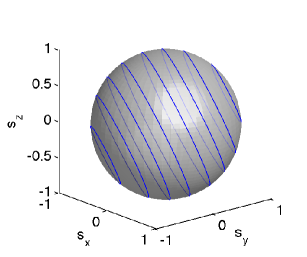
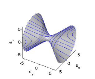
Figure 1: (colour online) Dynamical trajectories on the reduced state spaces. In the parameter region $u_{2}^{2}>u_{4}^{2}+u_{5}^{2}$ the reduced state space is just a two-sphere, upon which the dynamical equations (34) generate Rabi oscillations (left figure). In the parameter region $u_{2}^{2}<u_{4}^{2}+u_{5}^{2}$ the reduced state space is a two-dimensional hyperboloid, and the dynamical equations (41) generate open trajectories on this hyperbolic state space, if the energy eigenvalues are real (right figure). If the eigenvalues are complex, the open trajectories are rotated to form hyperbolic Rabi oscillations.

The evolution of the other dynamical variables $\sigma_{2},\sigma_{4},\sigma_{5}$ can be analysed as follows. Recall that the dynamics (34) preserves the relation (35). Thus, by subtracting (35) from (32) and rearranging terms we deduce that

$$-(u_{2}\sigma_{4}+u_{4}\sigma_{2})^{2}+(u_{4}\sigma_{5}-u_{5}\sigma_{4})^{2}-(u_{5}\sigma_{2}+u_{2}\sigma_{5})^{2}={\rm const}.$$ (36)

This shows that the evolution of the vector $(\sigma_{2},\sigma_{4},\sigma_{5})$ is confined to a hyperbolic cylinder. It turns out that the time evolution of these ‘hidden’ dynamical variables $\sigma_{2},\sigma_{4},\sigma_{5}$ can also be represented in a form similar to Bloch equations if we transform the variables according to $\sigma_{y_{1}}=u_{4}\sigma_{5}-u_{5}\sigma_{4}$, $\sigma_{y_{2}}=u_{5}\sigma_{2}+u_{2}\sigma_{5}$, and $\sigma_{y_{3}}=u_{2}\sigma_{4}+u_{4}\sigma_{2}$. In terms of these auxiliary variables we have

$$\mbox{$\textstyle\frac{1}{2}$}{\dot{\sigma}}_{y_{1}} = -\frac{u_{0}}{\nu}(u_{5}\sigma_{y_{2}}+u_{4}\sigma_{y_{3}})$$

$$\mbox{$\textstyle\frac{1}{2}$}{\dot{\sigma}}_{y_{2}} = -\frac{u_{0}}{\nu}(u_{2}\sigma_{y_{3}}+u_{5}\sigma_{y_{1}})$$ (37)

$$\mbox{$\textstyle\frac{1}{2}$}{\dot{\sigma}}_{y_{3}} = -\frac{u_{0}}{\nu}(u_{4}\sigma_{y_{1}}-u_{2}\sigma_{y_{2}}).$$

It should be evident that these dynamics are confined to a hyperboloid:

$$-\sigma_{y_{1}}^{2}+\sigma_{y_{2}}^{2}+\sigma_{y_{3}}^{2}={\rm const}.$$ (38)

Note, however, that when $u_{0}=0$ we have ${\dot{\sigma}}_{y_{1}}={\dot{\sigma}}_{y_{2}}={\dot{\sigma}}_{y_{3}}=0$ from (37), while $\sigma_{2},\sigma_{4},\sigma_{5}$ are in general evolving in time. Hence in transforming the variables into $\sigma_{y_{1}},\sigma_{y_{2}},\sigma_{y_{3}}$, part of the information concerning the dynamics is lost.

We see from (35) and (36) that on the ‘imaginary part’ of the state space the dynamics is endowed with hyperbolic characteristics, which nevertheless is not visible on the reduced state space, or the ‘real part’ of the state space $S^{2}$ spanned by $\sigma_{x},\sigma_{y},\sigma_{z}$.

When $u_{2}^{2}=u_{4}^{2}+u_{5}^{2}$ so that the imaginary part of the coquaternion appearing in the Hamiltonian is null, a calculation shows that the reduced spin variables obey the following dynamical equations:

$$\mbox{$\textstyle\frac{1}{2}$}{\dot{\sigma}}_{x} = -u_{3}\sigma_{y}$$

$$\mbox{$\textstyle\frac{1}{2}$}{\dot{\sigma}}_{y} = -u_{3}\sigma_{x}+u_{1}\sigma_{z}$$ (39)

$$\mbox{$\textstyle\frac{1}{2}$}{\dot{\sigma}}_{z} = u_{1}\sigma_{y},$$

and preserve $\sigma_{x}^{2}-\sigma_{y}^{2}+\sigma_{z}^{2}$.

When $u_{2}^{2}<u_{4}^{2}+u_{5}^{2}$ so that the imaginary part of the coquaternion in the Hamiltonian is space-like, the structure of the state space, as well as the dynamics, change, and they exhibit an interesting and nontrivial behaviour. The five-dimensional spin variables in this case evolve according to

$$\mbox{$\textstyle\frac{1}{2}$}{\dot{\sigma}}_{1} = -\nu\sigma_{3}-\frac{u_{3}}{\nu}(u_{2}\sigma_{2}+u_{4}\sigma_{4}+u_{5}\sigma_{5})$$

$$\mbox{$\textstyle\frac{1}{2}$}{\dot{\sigma}}_{2} = \frac{1}{\nu}(u_{2}u_{3}\sigma_{1}-u_{1}u_{2}\sigma_{3}+u_{0}u_{5}\sigma_{4}-u_{0}u_{4}\sigma_{5})$$

$$\mbox{$\textstyle\frac{1}{2}$}{\dot{\sigma}}_{3} = \nu\sigma_{1}+\frac{u_{1}}{\nu}(u_{2}\sigma_{2}+u_{4}\sigma_{4}+u_{5}\sigma_{5})$$ (40)

$$\mbox{$\textstyle\frac{1}{2}$}{\dot{\sigma}}_{4} = \frac{1}{\nu}(-u_{3}u_{4}\sigma_{1}+u_{0}u_{5}\sigma_{2}+u_{1}u_{4}\sigma_{3}+u_{0}u_{2}\sigma_{5})$$

$$\mbox{$\textstyle\frac{1}{2}$}{\dot{\sigma}}_{5} = \frac{1}{\nu}(-u_{3}u_{5}\sigma_{1}-u_{0}u_{4}\sigma_{2}+u_{1}u_{5}\sigma_{3}-u_{0}u_{2}\sigma_{4}),$$

where $\nu=\sqrt{u_{4}^{2}+u_{5}^{2}-u_{2}^{2}}$. These evolution equations preserve the normalisation (32). However, in the region $u_{2}^{2}<u_{4}^{2}+u_{5}^{2}$ the reduced spin variables $\sigma_{x},\sigma_{y},\sigma_{z}$ defined by (33) no longer obey the standard Bloch equations (34); instead, they satisfy

$$\mbox{$\textstyle\frac{1}{2}$}{\dot{\sigma}}_{x} = -\nu\sigma_{z}-u_{3}\sigma_{y}$$

$$\mbox{$\textstyle\frac{1}{2}$}{\dot{\sigma}}_{y} = -u_{3}\sigma_{x}+u_{1}\sigma_{z}$$ (41)

$$\mbox{$\textstyle\frac{1}{2}$}{\dot{\sigma}}_{z} = u_{1}\sigma_{y}+\nu\sigma_{x},$$

and preserve the relation

$$\sigma_{x}^{2}-\sigma_{y}^{2}+\sigma_{z}^{2}={\rm const}.$$ (42)

We thus see that at the level of reduced spin variables in three dimensions, the state space changes from a two-sphere (35) to a hyperboloid (42), as the parameters $u_{2},u_{4},u_{5}$ appearing in the Hamiltonian change. This transition corresponds to the transition from a complex Hermitian Hamiltonian into a PT-symmetric non-Hermitian Hamiltonian. Since the energy eigenvalues can still be real even when $u_{2}^{2}<u_{4}^{2}+u_{5}^{2}$, we expect the dynamics to exhibit two distinct characteristics depending on whether the reality condition $u_{1}^{2}+u_{2}^{2}+u_{3}^{2}>u_{4}^{2}+u_{5}^{2}$ is satisfied. Indeed, we found that on a hyperbolic state space, orbits of the unitary dynamics associated with real energies are the ones that are open and run off to infinities. Conversely, when the reality condition is violated, these open orbits are in effect Wick rotated to generate closed orbits. These features can be identified by a closer inspection on the structure of the underlying state space, upon which the dynamical orbits lie. In particular, (41) shows that the dynamics generates a rotation around the axis $(u_{1},\nu,u_{3})$; whereas the state space (42) is a hyperboloid about the axis $(0,1,0)$. We have sketched in figure 2 dynamical orbits resulting from (41), indicating that there indeed is a transition from open to closed orbits as real eigenvalues turn into complex conjugate pairs.

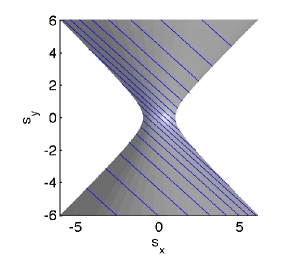
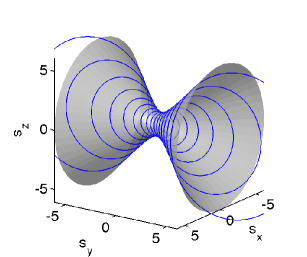
Figure 2: (colour online) Conic sections and PT phase transition: changes of orbit structures. A projection of the orbits on the hyperboloid, for parameters just above the transition to complex energy eigenvalues, is shown on the left side. The orbits form circular sections. On the right side we plot orbits of hyperbolic Rabi oscillations further into complex energy eigenvalues. The energy eigenvalues determine the angle between the axis of rotation and the axis of the hyperboloid. When eigenvalues are complex, the axis of rotation is within the hyperboloid, leading to closed orbits on the state space generated by circular sections. When the imaginary part of the coquaternion appearing in the Hamiltonian is null, we have parabolic sections of the hyperboloid; whereas when the energy eigenvalues are real, the angle of the two axes is larger than $\pi/4$, and open orbits are generated by hyperbolic sections.

Intuitively, one might have expected an opposite transition since in a PT-symmetric model of a spin-$\frac{1}{2}$ system the renormalised Bloch vectors on a spherical state space follow closed orbits when eigenvalues are real, whereas sinks and sources are created when eigenvalues become complex Graefe3 . The apparent opposite behaviour seen here is presumably to do with the facts that the underlying state space is hyperbolic, not spherical, and that no renormalisation is performed here. In figure 2 we have sketched some dynamical trajectories when energy eigenvalues are complex. A projection of the dynamical orbits from the $\sigma_{z}$ axis (for the choice of parameters used in these plots) shows in which way the topology of the orbits are affected by the reality of the energy eigenvalues.

The evolutions of the other dynamical variables $\sigma_{2},\sigma_{4},\sigma_{5}$ are confined to the space characterised by the relation

$$(u_{2}\sigma_{4}+u_{4}\sigma_{2})^{2}-(u_{4}\sigma_{5}-u_{5}\sigma_{4})^{2}+(u_{5}\sigma_{2}+u_{2}\sigma_{5})^{2}={\rm const}.,$$ (43)

instead of the relation (36) of the previous case. However, if we define, as before, three auxiliary variables $\sigma_{y_{1}}=u_{4}\sigma_{5}-u_{5}\sigma_{4}$, $\sigma_{y_{2}}=u_{5}\sigma_{2}+u_{2}\sigma_{5}$, and $\sigma_{y_{3}}=u_{2}\sigma_{4}+u_{4}\sigma_{2}$, then the dynamical equations satisfied by these variables are identical to those in (37), except, of course, that the definition of $\nu$ is different.

It is interesting to remark that when the imaginary part of the coquaternion appearing in the Hamiltonian is space-like, the imaginary unit ${\boldsymbol{i}}$ has the characteristic of a ‘double number’ or a ‘Study number’ introduced by Clifford Clifford , that is, ${\boldsymbol{i}}^{2}=1$. Quantum theories generated by such a number field (instead of the field of complex numbers) and other hyperbolic generalisations, as well as various issues that might arise from such generalisations, have been discussed by various authors (e.g., Hudson ; kocik1999 ; see also Kisil and references cited therein). The use of coquaternionic Hermitian Hamiltonian thus captures dynamical behaviours of different generalisations of quantum mechanics in a simple unified scheme.

We thank the participants of the international conference on Analytic and Algebraic Methods in Physics VII, Prague, 2011, for stimulating discussions. EMG is supported by an Imperial College Junior Research Fellowship.

References

(1) Bender, C. M., Boettcher S. & Meisinger, P. N.
1999 PT-symmetric quantum mechanics. J. Math. Phys.40, 2201.
(2)
Kaushal, R. S. & Korsch, H. J. 2000 Some remarks on complex
Hamiltonian systems. Phys. Lett. A276, 47.
(3)
Mostafazadeh, A. 2006 Real description of classical Hamiltonian
dynamics generated by a complex potential. Phys. Lett. A357,
177.
(4)
Bender, C. M., Holm, D. D. & Hook, D. W. 2007
Complex trajectories of a simple pendulum.
J. Phys. A40, F81.
(5)
Bender, C. M., Hook, D. W. & Kooner, K. S. 2010
Classical particle in a complex elliptic pendulum.
J. Phys. A43, 165201.
(6)
Cavaglia, A., Fring, A. & Bagchi, B. 2011
PT-symmetry breaking in complex nonlinear wave equations and their
deformations. arXiv:1103.1832
(7)
Bender, C. M. & Boettcher S. 1998
Real spectra in non-Hermitian Hamiltonians having PT symmetry.
Phys. Rev. Lett.80, 5243.
(8)
Lévai, G. & Znojil, M. 2000
Systematic search for PT-symmetric potentials with real energy spectra.
J. Phys. A33, 7165.
(9) Bender, C. M., Brody, D. C. & Jones, H. F. 2002
Complex extension of quantum mechanics.
Phys. Rev. Lett.89, 270401.
(10) Mostafazadeh, A. 2002 Pseudo-Hermiticity
versus PT-symmetry III: Equivalence of pseudo-Hermiticity and
the presence of antilinear symmetries. J. Math. Phys.43, 3944.
(11)
J. Okołowicz, J., Płoszajczak, M. & Rotter, I. 2003
Dynamics of quantum systems embedded in a continuum.
Phys. Rep.374, 271.
(12)
Jones, H. F. & Rivers, R. J. 2009
Which Green functions does the path integral for quasi-Hermitian
Hamiltonians represent?
Phys. Lett. A373, 3304.
(13)
Dorey, P., Dunning, C., Lishman, A. & Tateo, R. 2009
PT symmetry breaking and exceptional points for a class of inhomogeneous
complex potentials.
J. Phys. A42, 465302.
(14)
Witten, E. 2010
A new look at the path integral of quantum mechanics.
arXiv:1009.6032.
(15) Graefe, E. M., Korsch, H. J. &
Niederle, A. E. 2010 Quantum-classical correspondence for
a non-Hermitian Bose-Hubbard dimer. Phys. Rev.
A82, 013629.
(16)
Günther, U. & Kuzhel, S. 2010
PT symmetry, Cartan decompositions, Lie triple systems and Krein
space-related Clifford algebras. J. Phys. A43, 39002.
(17)
Moiseyev, N. 2011 Non-Hermitian Quantum Mechanics,
(Cambridge: Cambridge University Press).
(18) Nesterov, A. I. 2009 Non-Hermitian quantum
systems and time-optimal quantum evolution. SIGMA5, 069.
(19) Brody, D. C. & Graefe, E. M. 2011
On complexified mechanics and coquaternions. J. Phys.
A44, 072001.
(20) Finkelstein, D., Jaueh, J. M., Schiminovieh, S.
& Speiser, D. 1962 Foundations of quaternion quantum mechanics.
J. Math. Phys.3, 207.
(21) Adler, S. L. 1995 Quaternionic Quantum
Mechanics and Quantum Fields. (Oxford: Oxford University
Press).
(22) Brody, D. C. & Graefe, E. M. 2011
Six-dimensional space-time from quaternionic quantum mechanics.
arXiv:1105.3604.
(23)
Kisil, V. V. 2010
Erlangen programme at large 3.1: Hypercomplex representations of the
Heisenberg group and mechanics. arXiv:1005.5057v2
(24) Cockle, J. 1849 On systems of algebra
involving more than one imaginary. Phil. Magazine35, 434.
(25) Wang, Q., Chia, S., & Zhang, J. 2010 PT
symmetry as a generalisation of Hermiticity. J. Phys.
A43, 295301.
(26)
Clifford, W. K. 1878
Applications of Grassmann’s extensive algebra.
Am. J. Math.1, 350.
(27)
Hudson, R. L. 1966
Generalised translation-invariant mechanics.
D. Phil. Thesis, Bodleian Library, Oxford.
(28)
Kocik, J. 1999
Duplex numbers, diffusion systems, and generalized quantum mechanics.
Int. J. Theo. Phys.38, 2221.