Distance to Galactic globulars using the near-infrared magnitudes of RR Lyrae stars: IV. The case of M5 (NGC 5904)
Abstract
We present new and accurate near-infrared (NIR) , -band time series data for the Galactic globular cluster (GC) M5 = NGC 5904. Data were collected with SOFI at the NTT (71 120 images) and with NICS at the TNG (25 22 images) and cover two orthogonal strips across the center of the cluster of arcmin2 each. These data allowed us to derive accurate mean -band magnitudes for fundamental (RRab) and first overtone (RRc) RR Lyrae stars. Using this sample of RR Lyrae stars, we find that the slope of the -band Period Luminosity (PLK) relation () agrees quite well with similar estimates available in the literature. We also find, using both theoretical and empirical calibrations of the PLK relation, a true distance to M5 of mag. This distance modulus agrees very well (1) with distances based on main sequence fitting method and on kinematic method ( mag, Rees 1996), while is systematically smaller than the distance based on the white dwarf cooling sequence ( mag, Layden et al. 2005), even if with a difference slightly larger than 1. The true distance modulus to M5 based on the PLJ relation ( mag) is in quite good agreement with the distance based on the PLK relation further supporting the use of NIR PL relations for RR Lyrae stars to improve the precision of the GC distance scale.
keywords:
Stars:distances - Stars:horizontal branch - Galaxy:globular clusters:individual:M51 Introduction
Galactic Globular Clusters (GGCs) are crucial stellar systems to constrain the input physics adopted to construct evolutionary and pulsation models (Renzini & Fusi Pecci, 1988; Marconi et al., 2003; Cassisi, 2010), to investigate the kinematic properties of gas-poor, compact systems (Meylan & Heggie, 1997) and to constrain the formation and evolution of the Galactic spheroid (halo, thick disk, bulge; e.g. Mackey & van den Bergh 2005; Bica et al. 2006; Forbes & Bridges 2010). The GGCs often host RR Lyrae variables (RRLs), which are fundamental distance indicators for low-mass, old stellar populations. They are bright enough to have been detected in several Local Group galaxies (e.g. Dall’Ora et al. 2003, 2006; Pietrzyński et al. 2008; Greco et al. 2009; Fiorentino et al. 2010; Yang et al. 2010). They can also be easily identified, since they have characteristic light curves and periods. The most popular methods to estimate their distances are the visual magnitude – metallicity relation and the near-infrared (NIR) Period-Luminosity (PL) relation (e.g. Bono 2003; Cacciari & Clementini 2003). The reader interested in other independent approaches based on RRL to estimate stellar distances is referred to the thorough investigations by, e.g., Marconi et al. (2003); Di Criscienzo et al. (2004); Feast et al. (2008).
The visual magnitude – metallicity approach appears to be hampered by several theoretical and empirical uncertainties affecting both the zero-point and the slope (Bono et al., 2003). The NIR PL relation seems very promising, since it shows several indisputable advantages. Dating back to the seminal investigation by Longmore et al. (1986) it has been demonstrated on empirical basis that RRL do obey to a well defined -band PL relation. The key reason why the PL relation shows up in the NIR bands is mainly due to the fact that the bolometric correction in the NIR bands, in contrast with optical bands, steadily decreases when moving from hotter to cooler RRLs. This means that they become brighter as they get cooler. The pulsation periods –at fixed stellar mass and luminosity– become longer, since cooler RRLs have larger radii. The consequence is a stronger correlation between period and magnitude when moving from the - to the -band.
The advantages of using NIR PL relations to estimate distances are manifold.
i) Evolutionary and pulsation predictions indicate that the NIR PL
relations are minimally affected by evolutionary effects inside the RRL instability strip. The same outcome applies for the typical spread in mass inside the RRL instability strip (Bono et al., 2001, 2003). This means that individual RRL distances based on the NIR PL relations are minimally affected by systematics introduced by their intrinsic parameters and evolutionary status.
ii) Theory and observations indicate that fundamental (F or RRab) and first overtone (FO or RRc) RRL do obey independent NIR PL relations that are linear over the entire period range covered by F and FO pulsators.
The NIR PL relations together with the aforementioned features have also three positive observational advantages.
a) The NIR magnitudes are minimally affected by reddening uncertainties. This means that the RR Lyrae NIR PL relations can provide robust distance estimates for systems affected by differential reddening.
b) The luminosity amplitude in the NIR bands is at least a factor of 2-3 smaller than in the optical bands. Therefore, accurate estimates of the mean NIR magnitudes can be obtained with a modest number of observations. Moreover, empirical light curve templates (Jones et al., 1996) can be adopted to improve the accuracy of the mean magnitude even when only a single observation is available.
c) Thanks to the unprecedented effort by the 2MASS project (Skrutskie et al., 2006), accurate samples of local NIR standard stars are available across the sky. This means that both relative and absolute NIR photometric calibrations do not require supplementary telescope time.
The use of the NIR PL relations is also affected by four drawbacks.
– Empirical estimates of the slope of NIR PL relations show a significant scatter from cluster to cluster. They range from (IC Sollima et al. 2006) to (M, Sollima et al. 2006) and it is not clear yet whether this change is either intrinsic or caused by possible observational biases.
– Both theoretical and empirical investigations of the PLK show a not-negligible scatter of the zero point. This is a crucial point, as we plan to adopt the PLK as a tool to derive distances. Indeed, if we set as a reference and , the most robust absolute magnitude estimates range from (infrared flux method, Longmore et al. 1990) to (HB models, Catelan et al. 2004; empirical calibration Sollima et al. 2006), with intermediate values of (pulsational models Bono et al. 2001; HB models,Cassisi et al. 2004).
– Evolutionary and pulsation predictions indicate that the intrinsic spread of the NIR PL relations decreases as soon as either the metallicity or the HB-type of the Horizontal Branch (HB) is taken into account (Bono et al., 2003; Cassisi et al., 2004; Catelan et al., 2004; Del Principe et al., 2006). This means that accurate distance estimates of field RRLs do require an estimate of the metallicity. Moreover, no general consensus has been reached yet concerning the value of the coefficient of the metallicity term in the NIR Period-Luminosity-Metallicity (PLZ) relations. The current estimates for the -band range from (Sollima et al., 2006) to (Bono et al., 2003)
mag/dex based on cluster and field RRLs, respectively.
– The use of the template light curves does require for each object accurate estimates of B/V-band amplitudes and of the epoch of maximum.
To address these problems our group undertook a long-term project aimed at providing homogeneous and accurate NIR photometry for several GCs hosting sizable samples of RRLs and covering a wide range of metallicities. We have already investigated the old LMC cluster Reticulum (Dall’Ora et al., 2004, hereinafter paper I), the GGC M92 (Del Principe et al., 2005, hereinafter paper II) and Centauri (Del Principe et al., 2006, hereinafter paper III).
In this paper we present new results for the GGC M5 (NGC). This system is a typical halo globular cluster, and indeed, it is located at a distance of only from the Sun, from the Galactic Center, and above the Galactic disc (Zinn, 1985); its space motion is (Cudworth & Hanson, 1993). Moreover, it has a low reddening (, according to the Harris catalog, Harris 1996, and its new revision Harris 2010) and metal-intermediate composition, with estimates ranging from (Butler, 1975) to (Carretta et al., 2009). This cluster is a very good target to investigate the NIR PLZ relation, since it hosts a rich sample of RRLs ( in the 2002 release of the Clement’s on-line catalog, Clement et al. 2001). The RRab stars have an average period of , making M5 as one of the classical Oosterhoff type I clusters (Oosterhoff, 1939). It is located only two degrees from the celestial equator, and therefore, the search for cluster variables has been performed using telescopes from both hemispheres. According to Sawyer Hogg (1973) a total of variables were present in M5 and among them were RRLs. A significant fraction of these variables were discovered by Bailey & Pickering (1917) with the remaining stars identified by Oosterhoff (1941). The central regions of M5 have been surveyed photographically by Gerashchenko (1987) and Kravtsov (1988) who found an additional variables. Subsequently, Cohen & Matthews (1992) supplemented the catalog with five other variables, while Reid (1996) presented observations of RRLs, three of which were new discoveries. Brocato et al. (1996) added new variables located across the central regions of the cluster. More recent investigations by Sandquist et al. (1996) and Drissen & Shara (1998) identified previously unknown variables, while Kaluzny et al. (2000) and Caputo et al. (1999) identified new variables. We end up with a sample of variable stars, and among them are F and FO RRLs.
The paper is organized as follows: in Sec. 2 we discuss the observations and the strategy adopted to perform the photometry and to calibrate the data. The RRL properties and the approach adopted to determine their light curves are presented in Sec. 4, while in Sec. 5 we present the PLK and the PLJ relations. Finally, in Sec. 6, we summarize the current findings and briefly outline future perspectives.
2 Observations and data reduction
We collected and images in six different runs from February 2001 to March 2002 with SOFI@NTT/ESO111http://www.eso.org/sci/facilities/lasilla/instruments/sofi/
overview.html and and data in two runs in May 2005 and July 2005 with NICS@TNG222http://www.tng.iac.es/instruments/nics/. The SOFI data were collected in the large field mode with a pixel scale of arcsec/pixels and with a field of view of . NICS was also used in the large field mode, with pixel scale of arcsec/pixels and with a field of view of . For both instruments, observations were obtained of off-target fields for the sky subtraction.
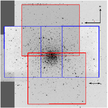
Since the cluster is moderately extended (tidal radius arcmin, Harris 2010), for both instruments two different pointings were observed, mapping the cluster in the North-South direction (SOFI) and in the East-West direction (NICS), covering two strips of about in both directions (see Fig. 1). We collected ( s of total exposure) - and ( s) -bands useful frames with SOFI, and ( s) - and ( s) -bands images with NICS. The number of epochs for recovered RRLs ranges from to . The log of observations is given in Table 1.
The raw SOFI frames were first corrected for the cross-talk effect with the IRAF333IRAF is distributed by the National Optical Astronomical Observatory, which is operated by the Association of Universities for Research in Astronomy, Inc., under cooperative agreement with the National Science Foundation. procedure crosstalk.cl, available in the SOFI web pages. Data were then pre-processed with our IRAF-based custom pipeline, which corrects for bias, flat field and bad pixel mask, and subtracts the sky contribution with a two-step technique as described in Pietrzyński & Gieren (2002). The NICS images were corrected for cross-talk with a FORTRAN program made available in the NICS web pages, and thereafter pre-processed with the same pipeline described above, without applying any bad pixel mask.
| DATE | INSTRUMENT | FILTER | EPOCHS | TOTAL EXP. TIME | SEEING (arcsec) |
|---|---|---|---|---|---|
| (sec) | (arcsec) | ||||
| 050201 | SOFI | 2 | 18 | 0.71 | |
| 2 | 120 | 0.74 | |||
| 070201 | SOFI | 2 | 18 | 0.74 | |
| 2 | 108 | 0.63 | |||
| 240202 | SOFI | 4 | 36 | 0.96 | |
| 4 | 228 | 0.75 | |||
| 250202 | SOFI | 6 | 54 | 0.66 | |
| 6 | 348 | 0.58 | |||
| 260202 | SOFI | 5 | 45 | 0.92 | |
| 5 | 300 | 0.93 | |||
| 090302 | SOFI | 6 | 57 | 0.72 | |
| 6 | 425 | 0.71 | |||
| 130505 | NICS | 2 | 105 | 0.50 | |
| 2 | 80 | 0.45 | |||
| 180705 | NICS | 2 | 88 | 0.66 | |
| 2 | 104 | 0.65 |
2.1 Photometry
For each image, a preliminary PSF model and a list of stars were produced with the DAOPHOTIV/ALLSTAR package (Stetson, 1987, 1994). In order to cross-match individual star catalogs, we computed geometric transformations with the DAOMATCH/DAOMASTER programs (Stetson, 1994), using as a reference a 2.2@MPG/ESO I-band image, available in the ESO data archive. A master star list was therefore produced on the total stacked image. We then performed a first ALLFRAME (Stetson, 1994) run, and a second star list was built on the median of the star-subtracted input images, which was merged with the previous one, in order to get a more complete input catalog. New accurate, spatially varying, PSF models were subsequently computed on the individual images, after cleaning each PSF star of contamination by faint neighbors, and a second ALLFRAME run was performed. We ended up with a final catalog of 38,131 sources.
2.2 Calibration
We calibrated each individual image to the Two Micron All Sky Survey (2MASS) photometric system, by selecting clean local 2MASS standards (i.e. bright and reasonably isolated, by taking advantage of the 2MASS photometric flags). The SOFI images collected before April 2003 are affected, due to the misalignment of the Large Field objective, by a strong distortion on a strip of pixels wide along the -axis. We found that the difference between instrumental and 2MASS magnitudes can attain values of the magnitudes in this region of the detector. Therefore, we wrote an ESO-MIDAS (Munich Image Data Analysis System) procedure to simultaneously correct for this positional effect and to get standard photometric zero-points. The procedure performs a polynomial regression of the instrumental magnitude as a function of the and 2MASS magnitude variables. The accuracy of the calibration, evaluated as the standard deviation of the fit, varies with the images from approximately to mag. We explicitly note that a spatially varying PSF might introduce a positional effect. However, to overcome this problem the selected PSF stars for each image are uniformly distributed across the frame. The difference between instrumental and 2MASS magnitudes in the region not affected by distortions is minimal. Therefore the positional effect seems to be caused by the objective misalignment.
We did not include color terms in the calibration, since they are negligible in the
range of colors of interest. The SOFI data have minimal color dependence, as shown in the
SOFI web
pages444http://www.eso.org/sci/facilities/lasilla/instruments/sofi/
inst/setup/Zero_Point.html,
while the NICS -band data typically have a non-negligible dependence on the color, which in the original transformation by Wainscoat & Cowie 1992 is given in terms of the color. In fact, by combining the transformation between
the and the standard filter in the Caltech photometric system
(CIT, Frogel et al. 1978), as described in Wainscoat & Cowie (1992), with the transformations
between the 2MASS and the CIT systems (Carpenter, 2001), we end up with the following transformation: .
Since the typical HB colors range from to , and considering that the RRL Instability Strip is confined to an even narrower color range, we conclude that the maximum systematic error is magnitudes.
3 The Color-Magnitude Diagram
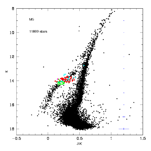
Fig. 2 shows the observed -() color-magnitude diagram. Stars plotted in this figure were selected by choosing only stars with small photometric contamination by close companions, using the SEPARATION index (Stetson et al., 2003). The contamination limit was set to , meaning that we selected only stars whose ratio (expressed in magnitudes) between the central surface brightness and the sum of the brightnesses of all other stars out to the FWHM is equal or larger than ( a factor of in flux). This means that we selected only stars whose correction for photometric contamination by other stars was smaller than . Since ALLFRAME fits the PSF model on each individual star when all the other stars in the image have been digitally subtracted, any uncorrected photometric contamination remaining should therefore be much smaller. We show only stars with estimated ALLFRAME photometric standard errors smaller than mag, both in the and band, corresponding to a signal-to-noise ratio on individual images of . Below this limit, we consider that the measurements on the individual images do not have sufficient accuracy to be included in our catalog. Adopting these cuts, we end up with star-like sources. Red and green filled circles represent RRab and RRc stars (see below), while cyan filled circles show variable stars excluded from the PLK and PLJ analysis (see Sec. 5). Our photometry covers the full range of magnitudes running from the Tip of the Red Giant Branch (RGB, ) down to magnitude below the Turn-Off (TO, ) region. The photometric limit can therefore be approximately located at mag, where the intrinsic photometric uncertainty is of the order of mag in the band. The CMD clearly shows the bump of the RGB, at mag, as well as the separation between the RGB and the Asymptotic Giant Branch (). The intrinsic features of the CMD and a comparison with evolutionary predictions will be addressed in a forthcoming paper.
4 RR Lyrae stars
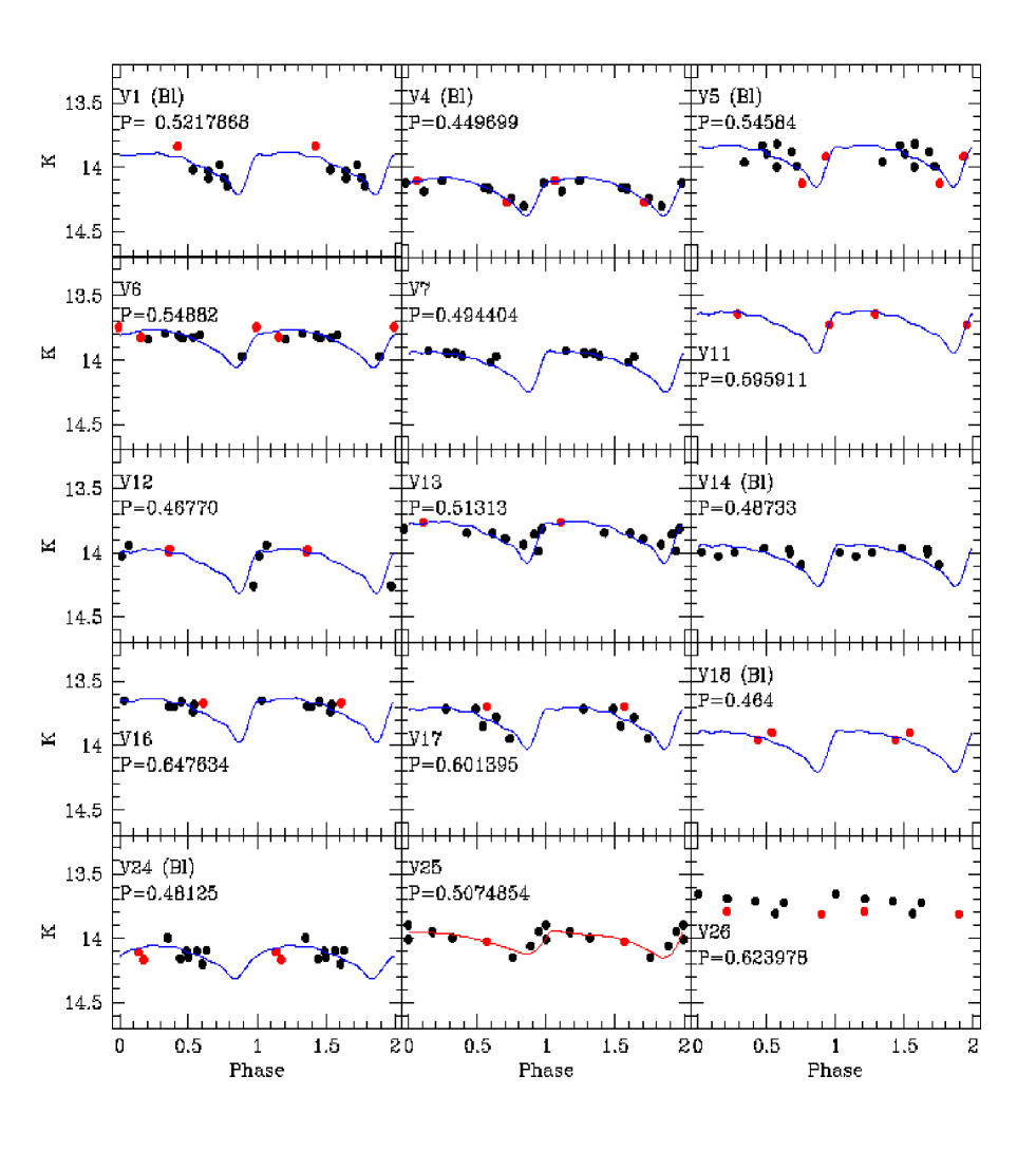
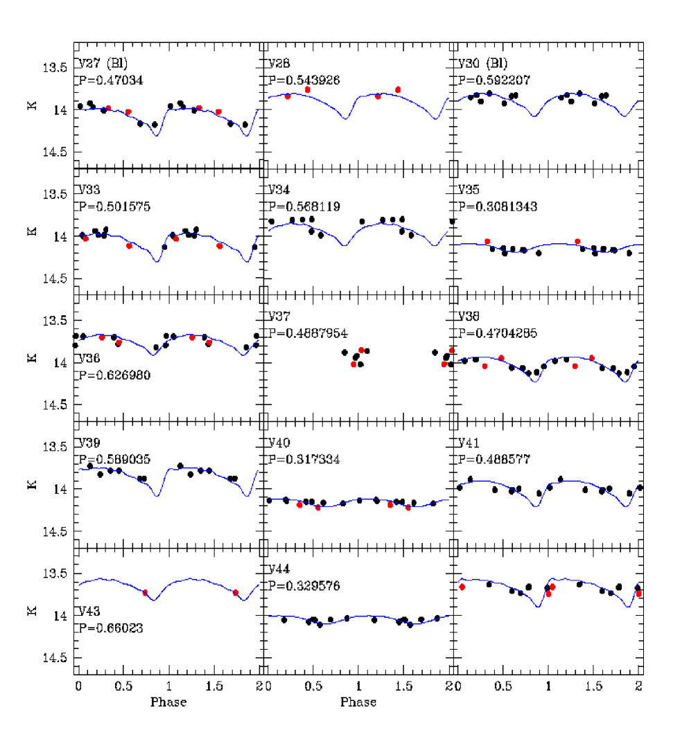
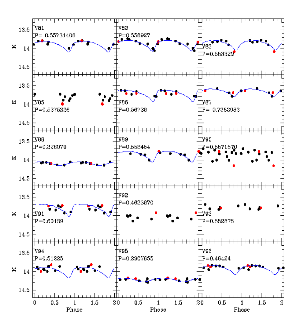
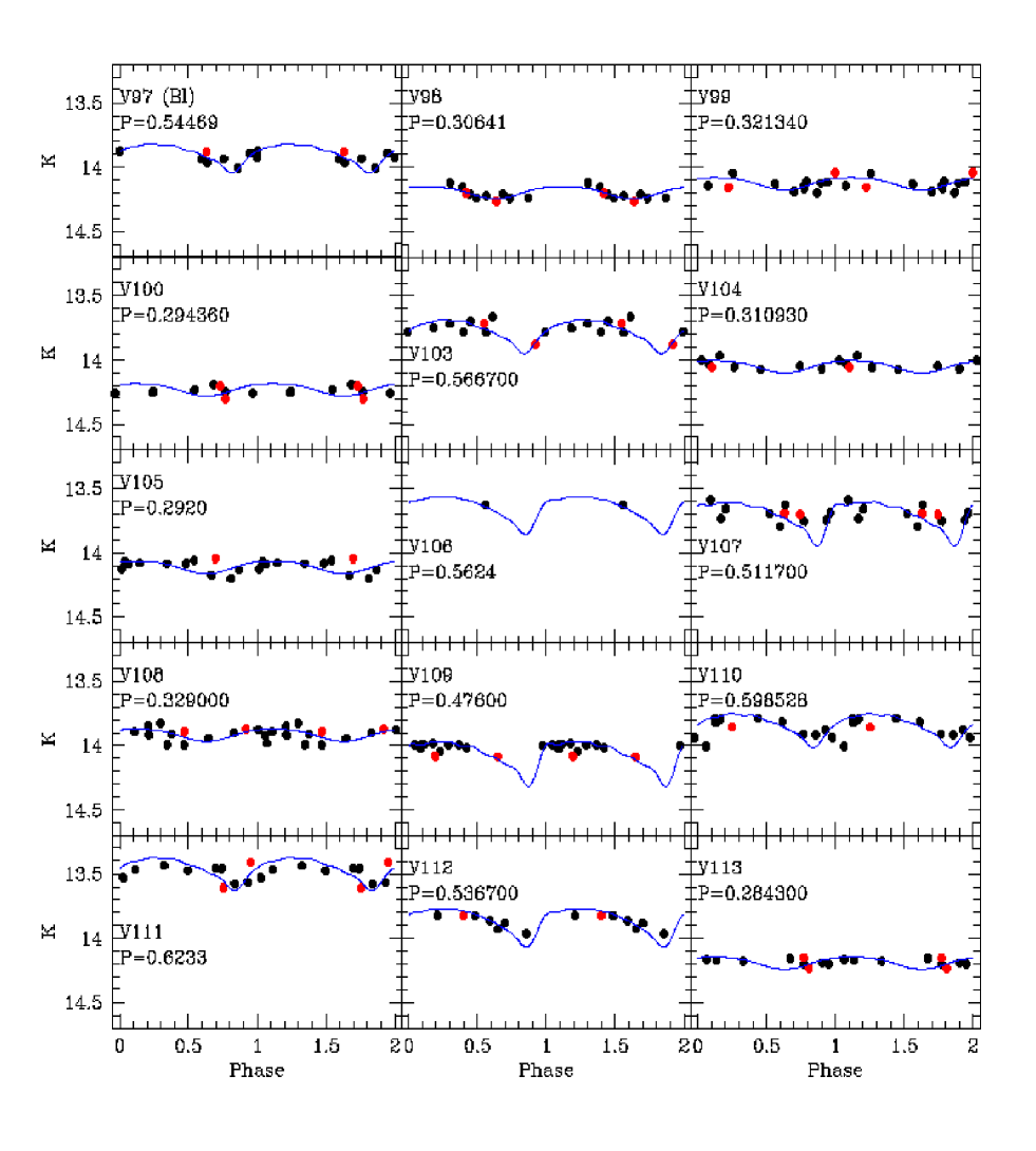
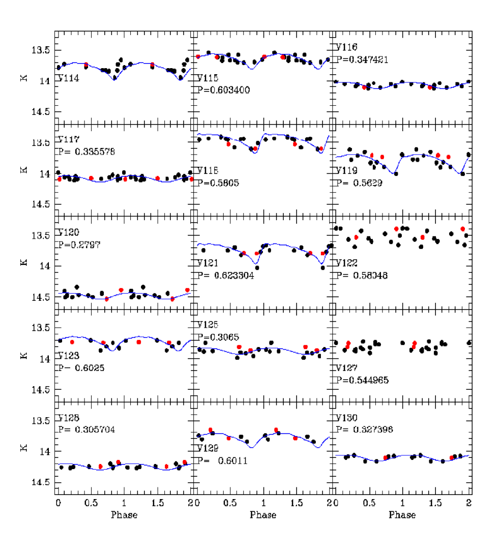
We recovered out of RR Lyrae variables on the basis of the WCS positions listed in the catalogs by Evstigneeva et al. (1999) and Samus et al. (2010). The RRLs not included in the current sample are located outside the region covered by our data. Barycentric Julian days were computed for each epoch of observation. The total exposure for each epoch was split into a number of shorter frames, and the final mean magnitude was estimated as an average of the measurements over all the individual frames. The -band light curves of RRLs are almost sinusoidal and the luminosity amplitude in this band is also modest. However, the most accurate results for the mean magnitudes are achieved by using the light curve templates provided by Jones et al. (1996). The use of the template yields accurate mean magnitudes even when only a single epoch is available. Note that the use of the template requires accurate ephemerides and -band amplitudes. Therefore, we mined the available literature to get updated periods, epochs of maxima and -band amplitudes. In most cases the -band amplitude was not available, and we transformed the -band amplitude into the -band one using the relation (Jones et al., 1996). Table 2 lists our adopted parameters: the name of the variable (following the number scheme proposed in Caputo et al. 1999), the adopted period with the related reference, the epoch of maximum with the associated reference, the computed intensity-averaged -band magnitude with the uncertainty , the variable type (fundamental, first overtone or Blazkho RRLs) and the -band amplitude , with the reference. For the Blazkho RRLs we follow the classification proposed by Jurcsik et al. (2010). Moreover, in several cases the period and the epoch of maximum were not available from the same reference, and we imposed a shift to the phased light curve to reasonably match the template. Shifts are listed in column of Table 2. Finally, column lists the adopted -band magnitude as extracted by the optical light curves of the unpublished archive of author PBS. In some cases the epoch was not available in literature and we used the epoch of our first measure to calculate the intensity-averaged -band magnitude. It is worth noting that period changes among the M5 RRLs have been detected by Storm et al. (1991); Reid (1996); Szeidl et al. (2010), but these changes are minimal and do not affect the conclusions of this investigation. An updated and homogeneous photometric catalog of the M5 RRLs is highly desirable. Note that RRLs for which the amplitude was not available in the literature were neglected. The intensity-weighted mean magnitudes –computed by DAOMASTER– of these objects are listed in column of Table 2. We also excluded a few variables that were heavily contaminated by bright neighbors or by close companions (see Sec. 4.1). The distance estimates based on the PLK relation rely on RRab and RRc variables. Some example of RRL light curves are depicted in Fig. 3. Black and red filled circles represent the SOFI and the NICS observations, respectively. The complete atlas of the light curves is available in the electronic version of this paper.
| Var | Period (Ref.) | Epoch (Ref.) | Type | AB (Ref.) | (V) | Note | |||
| [d] | (JD) | mag | mag | ||||||
| V1 | 0.5217868 (S10) | 48399.795 (R96) | 13.981 | 0.003 | Bl | 1.43 (K00) | -0.05 | 15.238 | no PLJ |
| V4 | 0.449699 (K00) | 48399.732 (R96) | 14.169 | 0.003 | Bl | 1.24 (K00) | -0.40 | 15.043 | |
| V5 | 0.54584 (R96) | 48399.787 (R96) | 13.920 | 0.003 | Bl | 1.42 (R96) | -0.05 | 15.188 | no PLJ |
| V6 | 0.54882 (R96) | 48399.743 (R96) | 13.853 | 0.002 | RRab | 1.18 (R96) | -0.30 | 15.225 | |
| V7 | 0.494404 (S91) | 46931.867 (S91) | 14.031 | 0.003 | RRab | 1.58 (S91) | +0.10 | 14.959 | no PLJ |
| V11 | 0.595911 (K00) | 48399.800 (R96) | 13.714 | 0.009 | RRab | 1.43 (K00) | +0.12 | 14.949 | no PLJ |
| V12 | 0.46770 (R96) | 48399.827 (R96) | 14.064 | 0.008 | RRab | 1.53 (R96) | 15.066 | no PLJ | |
| V13 | 0.51313 (R96) | 48424.744 (R96) | 13.848 | 0.003 | RRab | 1.40 (R96) | -0.40 | 14.861 | |
| V14 | 0.48733 (R96) | 48399.764 (R96) | 14.036 | 0.004 | Bl | 1.64 (R96) | -0.05 | 15.119 | |
| V16 | 0.647634 (K00) | 48400.734 (R96) | 13.730 | 0.003 | RRab | 1.53 (K00) | 14.887 | no PLJ | |
| V17 | 0.601395 (S10) | 52331.772* | 13.793 | 0.003 | RRab | 1.44 (S10) | -0.20 | 14.912 | |
| V18 | 0.464 (S91) | 46931.722 (S91) | 13.984 | 0.010 | Bl | 1.58 (K00) | 15.221 | no PLJ | |
| V24 | 0.48125 (R96) | 48400.702 (R96) | 14.139 | 0.003 | Bl | 0.96 (R96) | -0.10 | 14.983 | no PLJ |
| V25 | 0.5074854 (S10) | 51947.026* | 13.940 | RRab | 15.133 | ||||
| V26 | 0.623978 (S10) | 52331.892* | 13.71** | RRab | 14.973 | no PLK/PLJ | |||
| V27 | 0.47034 (R96) | 48404.890 (R96) | 14.074 | 0.002 | Bl | 1.44 (R96) | 14.994 | ||
| V28 | 0.543926 (S91) | 48400.710 (R96) | 13.925 | 0.012 | RRab | 1.25 (K00) | 15.075 | no PLJ | |
| V30 | 0.592207 (K00) | 46931.320 (S91) | 13.893 | 0.003 | Bl | 1.07 (K00) | -0.05 | 15.082 | no PLJ |
| V33 | 0.501575 (K00) | 48812.701 (R96) | 14.064 | 0.003 | RRab | 1.51 (K00) | 14.917 | ||
| V34 | 0.568119 (K00) | 48399.838 (R96) | 13.932 | 0.003 | RRab | 1.04 (K00) | +0.30 | 15.086 | no PLJ |
| V35 | 0.3081343 (S10) | 48400.745 (R96) | 14.131 | 0.003 | RRc | 0.61 (K00) | 15.009 | ||
| V36 | 0.626980 (R96) | 48400.818 (R96) | 13.746 | 0.003 | RRab | 0.81 (R96) | +0.20 | 15.041 | |
| V37 | 0.4887954 (S10) | 51946.869* | 13.94** | RRab | 15.049 | no PLK/PLJ | |||
| V38 | 0.4704285 (S10) | 48399.762 (R96) | 14.021 | 0.003 | RRab | 1.24 (R96) | +0.10 | 15.038 | |
| V39 | 0.589035 (K00) | 51946.751* | 13.845 | 0.003 | RRab | 1.51 (K00) | 15.116 | ||
| V40 | 0.317334 (K00) | 48424.744 (R96) | 14.157 | 0.003 | RRc | 0.57 (K00) | 15.067 | ||
| V41 | 0.488577 (K00) | 52331.697* | 13.995 | 0.003 | RRab | 1.37 (K00) | 15.239 | ||
| V43 | 0.66023 (R96) | 48424.762 (R96) | 13.648 | 0.026 | RRab | 0.89 (R96) | 15.093 | no PLJ | |
| V44 | 0.329576 (K00) | 48401.865 (R96) | 14.043 | 0.003 | RRc | 0.56 (K00) | 14.959 | ||
| V45 | 0.616595 (B96) | 48400.888 (R96) | 13.627 | 0.002 | RRab | 1.78 (B96) | 15.035 | ||
| V47 | 0.539739 (K00) | 48404.910 (R96) | 13.939 | 0.003 | RRab | 1.34 (K00) | 15.121 | ||
| V52 | 0.501785 (K00) | 48424.740 (R96) | 13.046 | 0.003 | Bl | 0.74 (R96) | 14.997 | ||
| V53 | 0.373594 (B96) | 51946.832* | 13.889 | 0.003 | RRc | 0.54 (B96) | 14.773 | ||
| V54 | 0.454239 (K00) | 48399.732 (R96) | 14.099 | 0.003 | RRab | 1.53 (K00) | +0.25 | 15.272 | |
| V55 | 0.3289023 (S91) | 46931.498 (S91) | 14.113 | 0.003 | RRc | 0.55 (S10) | 15.101 | ||
| V56 | 0.53468 (R96) | 48424.771 (R96) | 13.894 | 0.002 | Bl | 0.96 (R96) | -0.06 | 15.217 | |
| V57 | 0.284673 (K00) | 48399.770 (R96) | 14.289 | 0.003 | RRc | 0.65 (K00) | 14.995 | ||
| V59 | 0.542027 (K00) | 48399.740 (R96) | 13.908 | 0.004 | RRab | 1.28 (K00) | 0.15 | 15.031 | |
| V60 | 0.285274 (O99) | 51946.726* | 14.281 | 0.003 | RRc | 0.71 (S10) | 15.027 | ||
| V64 | 0.544492 (K00) | 51946.923* | 14.050 | 0.003 | RRab | 1.32 (K00) | 15.057 | ||
| V65 | 0.480758 (K00) | 48404.897 (R96) | 14.074 | 0.003 | Bl | 0.99 (R96) | -0.25 | 15.317 | no PLJ |
| V77 | 0.8451232 (K00) | 51946.954* | 13.450 | 0.011 | RRab | 0.79 (K00) | 14.706 | no PLJ | |
| V78 | 0.264798 (K00) | 48399.865 (R96) | 14.350 | 0.003 | RRc | 0.52 (K00) | 15.098 | ||
| V79 | 0.333089 (K00) | 48400.725 (R96) | 14.070 | 0.003 | RRc | 0.47 (K00) | 15.071 | ||
| V80 | 0.336549 (K00) | 48400.702 (R96) | 14.073 | 0.003 | RRc | 0.52 (K00) | 15.064 | ||
| V81 | 0.55731406 (B96) | 48399.764 (R96) | 13.893 | 0.002 | RRab | 1.21 (B96) | -0.30 | 15.080 | no PLJ |
| V82 | 0.558927 (K00) | 48399.791 (R96) | 13.866 | 0.003 | RRab | 1.19 (K00) | 15.055 | ||
| V83 | 0.553329 (R96) | 48399.805 (R96) | 13.862 | 0.002 | RRab | 1.09 (R96) | +0.25 | 15.085 | |
| V85 | 0.5275226 (S10) | 51946.869* | 13.75** | RRab | 14.861 | no PLK/PLJ | |||
| V86 | 0.56728 (B96) | 51947.124* | 13.717 | 0.003 | RRab | 1.57 (B96) | 14.731 | no PLK/PLJ-crowded | |
| V87 | 0.7383982 (S10) | 48400.841 (R96) | 13.651 | 0.003 | RRab | 0.49 (S10) | 14.922 | ||
| V88 | 0.328070 (K00) | 48404.910 (R96) | 14.092 | 0.003 | RRc | 0.57 (K00) | +0.25 | 14.940 | |
| V89 | 0.558454 (K00) | 48400.793 (R96) | 13.852 | 0.003 | RRab | 1.22 (K00) | +0.05 | 15.169 | |
| V90 | 0.5571570 (S10) | 51946.757* | 13.86** | RRab | 15.060 | no PLK/PLJ |
| Var | Period (Ref.) | Epoch (Ref.) | Type | AB (Ref.) | (V) | Note | |||
| [d] | (JD) | mag | mag | ||||||
| V91 | 0.60139 (R96) | 48401.834 (R96) | 13.787 | 0.003 | RRab | 1.44 (R96) | -0.05 | 15.125 | |
| V92 | 0.4633870 (S10) | 51946.684* | 13.99** | RRab | 15.199 | no PLK/PLJ | |||
| V93 | 0.552875 (O99) | 51946.814* | 13.73** | RRab | 14.967 | no PLK/PLJ | |||
| V94 | 0.51225 (R96) | 48424.788 (R96) | 13.971 | 0.003 | RRab | 1.22 (R96) | 15.107 | no PLJ | |
| V95 | 0.2907655 (S10) | 52331.021* | 14.222 | 0.003 | RRc | 0.66 (S10) | 15.037 | ||
| V96 | 0.46424 (R96) | 48399.806 (R96) | 13.915 | 0.003 | RRab | 0.86 (R96) | +0.40 | 15.079 | no PLK/PLJ-crowded |
| V97 | 0.54469 (R96) | 48399.850 (R96) | 13.891 | 0.002 | Bl | 0.67 (R96) | 15.000 | no PLJ | |
| V98 | 0.30641 (B96) | 51946.870* | 14.190 | 0.003 | RRc | 0.68 (S10) | 14.958 | no PLJ | |
| V99 | 0.321340 (R96) | 48401.921 (R96) | 14.120 | 0.003 | RRc | 0.61 (R96) | 14.907 | ||
| V100 | 0.294360 (R96) | 48399.761 (R96) | 14.224 | 0.004 | RRc | 0.72 (R96) | 15.061 | ||
| V103 | 0.5667 (C99) | 47629.551 (C99) | 13.771 | 0.003 | RRab | 1.03 (C99) | -0.36 | 15.019 | |
| V104 | 0.310930 (O99) | 52331.862* | 14.044 | 0.003 | RRc | 0.9 (C99) | 15.048 | no PLK/PLJ | |
| V105 | 0.2920 (C99) | 47629.813 (C99) | 14.107 | 0.007 | RRc | 0.94 (C99) | 14.882 | ||
| V106 | 0.5624 (C99) | 47629.311 (C99) | 13.652 | 0.007 | RRab | 1.20 (C99) | 0.05 | 14.804 | no PLK/PLJ-crowded |
| V107 | 0.5117 (C99) | 47629.776 (C99) | 13.703 | 0.005 | RRab | 1.52 (C99) | 14.767 | no PLK/PLJ-crowded | |
| V108 | 0.329 (C99) | 51946.902* | 13.913 | 0.004 | RRc | 0.55 (C99) | 14.802 | no PLK/PLJ-blended? | |
| V109 | 0.476 (C99) | 47629.854 (C99) | 14.069 | 0.003 | RRab | 1.55 (C99) | 15.127 | no PLJ | |
| V110 | 0.598528 (O99) | 51946.779* | 13.838 | 0.003 | RRab | 0.95 (C99) | 15.218 | ||
| V111 | 0.6233 (C99) | 47629.283 (C99) | 13.456 | 0.009 | RRab | 0.93 (C99) | 15.018 | no PLK/PLJ-crowded | |
| V112 | 0.5367 (C99) | 47629.546 (C99) | 13.858 | 0.003 | RRab | 1.29 (C99) | 14.941 | ||
| V113 | 0.2843 (C99) | 47629.758 (C99) | 14.185 | 0.003 | RRc | 0.70 (C99) | 14.913 | ||
| V114 | 0.604015 (O99) | 47629.573 (C99) | 13.794 | 0.003 | RRab | 1.08 (C99) | 15.120 | ||
| V115 | 0.6034 (C99) | 47629.772 (C99) | 13.639 | 0.003 | RRab | 0.77 (C99) | 14.954 | no PLK/PLJ-crowded | |
| V116 | 0.347421 (O99) | 47629.518 (C99) | 14.071 | 0.003 | RRc | 0.59 (C99) | +0.40 | 14.787 | |
| V117 | 0.335578 (O99) | 47629.520 (C99) | 14.077 | 0.003 | RRc | 0.53 (C99) | -0.48 | 14.895 | |
| V118 | 0.5805 (C99) | 47629.832 (C99) | 13.454 | 0.004 | RRab | 1.57 (C99) | -0.10 | 14.693 | no PLK/PLJ |
| V119 | 0.5629 (C99) | 47629.297 (C99) | 13.783 | 0.003 | RRab | 1.25 (C99) | +0.20 | 14.935 | |
| V120 | 0.2797 (C99) | 47629.698 (C99) | 14.474 | 0.004 | RRc | 0.71 (C99) | +0.10 | 15.018 | no PLK/PLJ-crowded |
| V121 | 0.623304 (B96) | 47629.303 (C99) | 13.733 | 0.003 | RRab | 1.69 (C99) | +0.05 | 14.846 | |
| V122 | 0.58048 (Cl) | 51946.869* | 13.47** | RRab | 14.611 | no PLK/PLJ | |||
| V123 | 0.6025 (C99) | 47629.303 | 13.715 | 0.003 | RRab | 0.65 (C99) | -0.10 | 14.989 | |
| V125 | 0.3065 (C99) | 47629.592 (C99) | 13.868 | 0.005 | RRc | 0.65 (C99) | 14.933 | no PLK/PLJ-crowded | |
| V127 | 0.544965 (O99) | 51946.869* | 13.80** | RRab | 15.059 | no PLK/PLJ | |||
| V128 | 0.305704 (O99) | 47629.785 (C99) | 14.240 | 0.003 | RRc | 0.68 (C99) | 14.904 | ||
| V129 | 0.6011 (C99) | 47629.631 (C99) | 13.783 | 0.003 | RRab | 0.74 (C99) | 15.112 | ||
| V130 | 0.327396 (R96) | 47581.469 (C99) | 14.100 | 0.003 | RRc | 0.50 (R96) | +0.46 | 14.887 | |
| V131 | 0.281521 (R96) | 47629.763 (C99) | 14.286 | 0.003 | RRc | 0.68 (C99) | +0.30 | 15.157 | |
| V132 | 0.2835 (C99) | 47629.648 (C99) | 14.255 | 0.004 | RRc | 0.49 (C99) | +0.20 | 14.974 | |
| V133 | 0.294905 (Cl99) | 52331.804* | 14.14** | RRc | 14.869 | no PLK/PLJ | |||
| V137 | 0.591 (C99) | 47629.520 (C99) | 13.825 | 0.003 | RRab | 0.60 (C99) | +0.20 | 15.020 | |
| V139 | 0.300 (C99) | 47629.587 (C99) | 14.186 | 0.003 | RRc | 0.42 (C99) | 14.946 | ||
| V142 | 0.4577 (C99) | 47629.830 (C99) | 14.078 | 0.003 | RRab | 1.5 (C99) | 15.194 | no PLJ | |
| V155 | 0.33 (DS) | 52331.827* | 14.101 | RRc | 14.882 | no PLK/PLJ | |||
| V156 | 0.47 (DS) | 51946.869* | 12.73** | RRab | 14.984 | no PLK/PLJ-blended? | |||
| V158 | 0.45 (DS) | 51947.004* | 13.58** | RRab | 14.235 | no PLK/PLJ | |||
| V161 | 0.331570 (O99) | 51946.736* | 14.035 | RRc | 15.051 | no PLK/PLJ | |||
| V162 | 0.557468 (O99) | 51946.925* | 13.86** | RRab | 15.060 | no PLK | |||
| V163 | 0.600853 (O99) | 52331.773* | 13.86** | RRab | 14.912 | no PLK | |||
| Epoch of our first measurement. | |||||||||
| Intensity-weighted mean magnitude computed by DAOMASTER. | |||||||||
| References: | |||||||||
| S91: Storm et al. (1991). | |||||||||
| B96: Brocato et al. (1996). | |||||||||
| R96: Reid (1996). | |||||||||
| DS: Drissen & Shara (1998). | |||||||||
| C99: Caputo et al. (1999). | |||||||||
| O99: Olech et al. (1999). | |||||||||
| K00: Kaluzny et al. (2000). | |||||||||
| S10: Szeidl et al. (2010). | |||||||||
4.1 Notes on individual variables
V25: for this variable we did not find any amplitude information in the literature. However since the pulsation cycle was evenly covered, we fitted the observed data with a spline curve, getting a light curve (red curve in Fig. 3) with a shape very similar to the template available for similar periods.
V84: actually this variable is a type II Cepheid, whose -band light curve was presented by Matsunaga et al. (2006), and it is included in our photometric catalog. Unfortunately, most of our measurements of this star are above the non-linearity level, and we were not able to produce a reliable light curve.
V86: this variable is heavily contaminated by close neighbors.
V96: this variable is heavily contaminated by close neighbors.
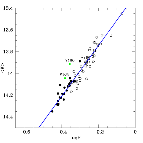
V104: this variable has been claimed to be a RRab variable by Reid (1996), but Drissen & Shara (1998) reported it as an eclipsing binary. We found that this variable does not fit the PLK relation (see Fig. 10), since its magnitude is mag brighter than the expected magnitude for its period, while the observed dispersion of the PLK relation is mag at the level. This gives support to the Drissen & Shara (1998) interpretation, as also stated in Caputo et al. (1999). However, Olech et al. (1999) reported this star as a multiperiodic variable, with a first overtone radial pulsation and a second period connected with non-radial pulsation.
V106: this variable is heavily contaminated by close neighbors.
V107: this variable is heavily contaminated by close neighbors.
V108 this variable appears to be overluminous in the PLK plane (see Fig. 10), and both overluminous and redder than expected from its pulsation period in the CMD (magenta point in Fig. 2). We therefore suspect that this variable is blended with a red companion, and we excluded it from our analysis.
V111: this variable is heavily contaminated by close neighbors.
V113: according to Caputo et al. (1999) this variable shows a () color significantly bluer than the blue limit of the instability strip, but with a luminosity which agrees with the average luminosity of the other variables. Excluding subtle effects of blending or crowding, the blue color remains unexplained. However, we found that this variable fairly matches the PLK relation and we used it in our analysis.
V115: this variable is heavily contaminated by close neighbors.
V118: this variable appears to be over-luminous in the PLK plane (green point in Fig. 10), and it has not been used for our PLK analysis. Since it does not seem to be blended, its over-luminosity in the -band is unexplained. We therefore dropped this star from the present study.
V120: this variable is heavily contaminated by close neighbors.
V125: this variable is heavily contaminated by close neighbors.
V156: this variable appears both overluminous and red in the CMD. We therefore suspected that this variable is blended with a red companion, and we excluded it from our analysis. In Fig. 3 we plot this variable after shifting the magnitude by 1 mag, to preserve the readability of the figure.

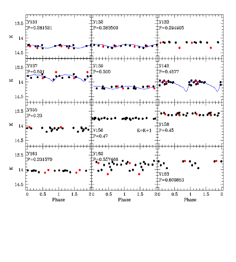
The -band magnitudes of V156 have been artificially shifted by 1 mag to make more clear the figure.
5 The PLK and the PLJ relations
In the following we compare our data with the available PLK calibrations, which can be divided into three broad groups: pulsational (Bono et al. 2001; Bono et al. 2003), synthetic (Cassisi et al. 2004; Catelan et al. 2004) and empirical (Sollima et al. 2006) PLK relations. We also compare our data with the PLJ calibration provided by Catelan et al. 2004.
Fig. 10 shows the observed mean -band magnitudes of the detected variables as a function of the period (observed PLK relation), the empirical fit (rms) to the data (blue line) is
| (1) |
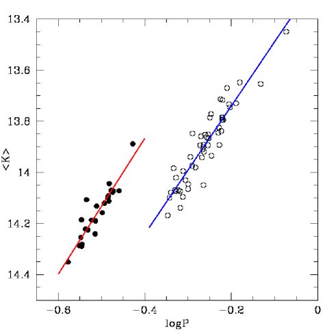
obtained fundamentalizing the first overtone pulsators (filled circles) by applying the relation (Di Criscienzo et al., 2004), to use the same PLK relation for fundamental (open circles) and first overtone pulsators. We remark that this offset is consistent with that implied by the difference in at costant in Fig. 10. The slope in Eq. 1 is consistent within with the empirical values found for this cluster ( Longmore et al. 1990; Sollima et al. 2006, unfortunately without uncertainty). Observed mean -band magnitudes of Rab and RRc are shown separately as a function of the period in Fig. 11. Symbols are the same of Fig. 10. Solid blue and red lines show the empirical fits to the RRab and RRc variables, respectively, in particular for the RRab variables:
| (2) |
and for RRc:
| (3) |
By adopting the theoretical calibration of Bono et al. (2001) (their eq. ) and a metallicity of (Kraft & Ivans, 2003), we can determine the individual distance moduli of the RRLs. The observations were transformed into the Bessell & Brett (1988) homogenized Johnson-Cousins-Glass photometric system according to the relation provided by Carpenter (2001). The weighted average of these estimates gives an apparent distance modulus , where the adopted uncertainty is the standard deviation (rms). The adopted reddening toward M5 is , as taken from the Harris (2010) catalog. We combine this value with the reddening law from Cardelli et al. (1989) of which gives an absorption in the -band of mag. Correcting the distance modulus for the reddening, we find that the true value is . These results indicate that the current distance estimate to M5 is minimally affected by reddening uncertainties and by uncertainties in the extinction law (McCall 2004; Bono et al. 2010).
In order to improve the theoretical calibration of the PLZK relation, Bono et al. (2003) devised a new pulsation approach that relies on mean -band magnitudes and () colors. In particular, they derived new period-luminosity-color-metallicity relations for RRab and RRc variables (see their relations and ) that include the luminosity term. According to these relations, one finds that accurate , photometric measurements of both RRab and RRc variables provide excellent proxies for the effective temperature, and can in turn be adopted to estimate the luminosity level. We therefore adopted accurate -band magnitudes extracted by optical light curves of the PBS unpublished archive (shown in the last column of Table 2) and we compared our empirical slopes in Eqs. 2 and 3 with the theoretical predictions, being and for RRab and RRc stars, respectively. Once we transform the observations into the Bessell & Brett (1988) system and after correcting for the reddening, we find a value of using the RRab stars, while using the RRc stars we find . Note that the dispersion of the distance estimates based on RRc stars is almost a factor of two smaller than the distance based on RRab stars, because the width in temperature of the region of the instability strip in which the FOs are pulsationally stable is typically a factor of two narrower than for the Fs. This means that the intrinsic dispersion in the infrared luminosity of FOs is systematically smaller than for Fs.
The evolutionary calibrations by Cassisi et al. (2004) and Catelan et al. (2004) are based on the Horizontal Branch morphology and on the RRL pulsational properties. These authors provide period-luminosity relations in the Johnson-Cousins-Glass photometric system, with slopes and zero-points that vary with the HB morphology and with the metallicity. In particular, Cassisi et al. (2004) gives a grid of slopes and zero-points as a function of the metallicity (expressed as the mass fraction ) and the HB type (HBT, according to the Lee, Demarque & Zinn parameter, Lee et al. 1994). We chose, among the values available in their published grid, and HBT since these parameters are those closest to the M5 literature values (HBT , taken from the Harris 2010 catalog), obtaining the calibration . Once we apply the correction for the difference in the photometric system and for the reddening, and having fundamentalized RRc variables, we find a true distance modulus to M5 of .
A very similar approach was devised by Catelan et al. (2004) who provided average relations, to be used when the HB type is not known a priori. However, we adopted their calibration with and HBT , obtaining the calibration . Again, once we apply the correction for the difference in the photometric system and for the reddening, and having fundamentalized the RRc variables, we found a true distance modulus to M5 of .
Finally, we also adopted the empirical calibration by Sollima et al. (2006) () and we found a true distance modulus of . It is interesting to note that Sollima et al. (2006), using a collection of data for RRLs, found a true distance to M5 () that agrees well with the current estimates.
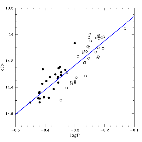
We end this section with a discussion of the observed PLJ relation. Fig. 12 shows observed
mean magnitudes of the considered RRLs vs. . The variables have been fundamentalized.
Since in the literature there are no suitable templates to adopt, and since the uneven phase coverage of the
observations did not allow us to interpolate the observed data with spline curves, we simply used
intensity-weighted mean magnitudes, as computed with DAOMASTER. To reduce subtle effects for uneven light curve sampling, we used for the PLJ only stars with a good phase coverage, therefore ending up with RRab and RRc stars. The observed slope is , which is in very good agreement with the available theoretical calibration (, Catelan et al. 2004). In passing, we note that F and FO pulsators seem to not follow a common relation even after fundamentalization, with the F variables alone apparently following a steeper distribution. On the other hand, we point out that the Catelan et al. 2004 calibration used as reference is obtained by using both and stars.
We transformed the observations in the Bessell & Brett (1988) homogenized Johnson-Cousins-Glass system with the relation , derived following the Carpenter (2001) equations. After correcting for the extinction with the Cardelli et al. (1989) law, we get a true PLJ-based distance to M5 of , in agreement with the PLK calibrations. We explicitly note that the distances based on the two PLK and PLJ calibrations provided by Catelan et al. (2004) are slightly longer than the others, but with an excellent internal agreement.
All predicted and empirical slopes and the distance moduli based on the above relations are listed in Table 4.
| Calibration | Predicted slope | Sample | Our Empirical slope | Our Empirical slope | DM0 (mag) |
|---|---|---|---|---|---|
| Bono et al. (2001) | -2.031 | F FO | – | -2.33 0.08 | 14.41 0.06 |
| Bono et al. (2003) | -2.102 | F | — | -2.50 0.14 | 14.46 0.09 |
| Bono et al. (2003) | -2.265 | FO | — | -2.66 0.23 | 14.46 0.05 |
| Cassisi et al. (2004) | -2.34 | FFO | — | -2.33 0.08 | 14.41 0.05 |
| Catelan et al. (2004) | -2.355 | FFO | — | -2.33 0.08 | 14.48 0.05 |
| Catelan et al. (2004) | -1.773 | FFO | -1.85 0.14 | — | 14.50 0.08 |
| Sollima et al. (2006) | -2.38 | FFO | — | -2.33 0.08 | 14.41 0.05 |
| Study | Method | [Fe/H] | Reddening | DM0 (mag) |
|---|---|---|---|---|
| Sollima et al. (2006) | PLK | |||
| Reid (1998) | Main sequence fitting | |||
| Carretta et al. (2000) | Main sequence fitting | |||
| Layden et al. (2005) | Main sequence fitting | |||
| Storm et al. (1994) | Baade-Wesselink | |||
| Di Criscienzo et al. (2004) | RRL pulsation properties | |||
| Rees (1996) | Proper motions | … | … | |
| Layden et al. (2005) | White dwarf fitting |
6 Discussion
On the basis of our data, we found that the weighted mean of the different theoretical and empirical calibrations of the PLK relation gives a true distance modulus of mag.
The distance to M5 based on the PLK relation also agrees quite well with similar estimates available in the literature, but based on different distance indicators. The distance estimates listed in Table 5 indicate quite clearly that the current distance agrees within with distance based not only on the PLK relation ( mag Sollima et al., 2006), but also on main-sequence fitting method (Reid, 1998; Carretta et al., 2000; Layden et al., 2005) and semi-geometric approach ( mag Storm et al., 1994). On the other hand, our distance is systematically longer than the distance to M5 provided by Di Criscienzo et al. (2004) using synthetic horizontal branch models and pulsation properties of RRLs and the difference is larger than 1.
In this context it is noteworthy that the distance based on the PLK relation agrees with the distance based on the proper motions = mag by Rees (1996). Even though the intrinsic error of the quoted distance estimates differ by more than one order of magnitude, the two distances taken at face value agree quite well. If this agreement is not fortuitous, due to the large error bar in the Rees (1996) estimate, this would be first time that kinematic distances agree with other distance indicators. Typically, the kinematic distances to GCs are 0.2-0.3 magnitudes smaller than distance moduli based either on the PLK relation of RRLs, or on main-sequence fitting, or on the tip of the Red Giant Branch (TRGB, Bono et al. 2008). The reasons for such discrepancies are not clear yet, but the current agreement appears very promising to further constrain the occurrence of possible systematic errors.
On the other hand, the distance based on the fitting of the White dwarf cooling sequence = mag provided by Layden et al. (2005) is approximately 0.2 mag larger than distances based on other methods. The difference with the distance based on the PLK relation and on main-sequence fitting is on average slightly larger than 1. This is also an interesting occurrence, since distance moduli to GCs based on the fitting of the white-dwarf cooling sequence are typically 0.1-0.3 mag smaller than distances to GCs based either on the TRGB, or on the PLK relation or on the main sequence fitting (Bono et al., 2008; Moehler & Bono, 2008).
We have also investigated the PLJ relation of RRL stars in M5, and from a sample of 35 RRab and 23 RRc (fundamentalized) variables we found an empirical slope of . The uncertainty in the slope of the PLJ relation is almost a factor of two larger than the uncertainty in the slope of the PLK relation (0.14 vs 0.08) because the luminosity amplitude in the -band is larger in the -band, and also because we still lack accurate -band light curve templates. Therefore, the mean -band magnitudes were estimated as a time average and only for RRLs with good phase coverage. Homogeneous sets of time series data both in and are required to constrain on an empirical basis the intrinsic spread of PLK and PLJ relations. Finally, we mention that by adopting the calibration of the PLJ relation provided by Catelan et al. (2004), we found a true distance modulus to M5 of mag. The distances based on the PLJ and on the PLK relations agree quite well, but the intrinsic error of the former is a factor of two larger.
The distances to M5 based either on the PLK or on the PLJ relation agree quite well with distances based on independent robust standard candles. This finding further supports the key role that accurate NIR photometry of cluster variables (RRL, type II Cepheids) can play in the improvement of GC distance scale (Matsunaga et al., 2010). Moreover and even more importantly, the comparison with M5 distances based on different distance indicators strongly supports the evidence that M5 might be a fundamental laboratory to constrain on a quantitative basis the thorny systematic uncertainties that might affect the most popular primary distance indicators. It goes without saying that this sanity check would benefit by further improvements in the precision of the kinematic distances and/or in the geometrical distances based on possible eclipsing binary systems in M5.
In a future paper we plan to compare optical and NIR photometry of M5 with evolutionary predictions, in particular for advanced evolutionary phases.
Acknowledgments
We sincerely thank an anonymous referee for her/his helpful comments, which improved the readibility of the paper.
GC is supported by the Italian Ministry of Education, University and Research (MIUR) grant PRIN-MIUR 2007:Multiple stellar populations in globular clusters: census, characterization and origin P.I.: G. Piotto.
This research has
made use of the SIMBAD data base, operated at CDS, Strasbourg,
France. This publication makes use of data products from the Two
Micron All Sky Survey, which is a joint project of the University of Massachusetts and the Infrared Processing and Analysis
Center/California Institute of Technology, funded by the National
Aeronautics and Space Administration and the National Science
Foundation.
References
- Bailey & Pickering (1917) Bailey, S. I., & Pickering, E. C. 1917, Annals of Harvard College Observatory, 78, 99
- Bessell & Brett (1988) Bessell, M. S., & Brett, J. M. 1988, PASP, 100, 1134
- Bica et al. (2006) Bica, E., Bonatto, C., Barbuy, B., & Ortolani, S. 2006, A&A, 450, 105
- Bono et al. (2001) Bono, G., Caputo, F., Castellani, V., Marconi, M., & Storm, J. 2001, MNRAS, 326, 1183
- Bono (2003) Bono, G. 2003, Stellar Candles for the Extragalactic Distance Scale, 635, 85
- Bono et al. (2003) Bono, G., Caputo, F., Castellani, V., Marconi, M., Storm, J., & Degl’Innocenti, S. 2003, MNRAS, 344, 1097
- Bono et al. (2008) Bono, G., et al. 2008, ApJL, 686, L87
- Bono et al. (2010) Bono, G., et al. 2010, ApJL, 708, L74
- Brocato et al. (1996) Brocato, E., Castellani, V., & Ripepi, V. 1996, AJ, 111, 809 (B96)
- Butler (1975) Butler, D. 1975, ApJ, 200, 68
- Cacciari & Clementini (2003) Cacciari, C., & Clementini, G. 2003, Stellar Candles for the Extragalactic Distance Scale, 635, 105
- Caputo et al. (1999) Caputo, F., Castellani, V., Marconi, M., & Ripepi, V. 1999, MNRAS, 306, 815 (C99)
- Cardelli et al. (1989) Cardelli, J. A., Clayton, G. C., & Mathis, J. S. 1989, ApJ, 345, 245
- Carpenter (2001) Carpenter, J. M. 2001, AJ, 121, 2851
- Carretta et al. (2000) Carretta, E., Gratton, R. G., Clementini, G., & Fusi Pecci, F. 2000, ApJ, 533, 215
- Carretta et al. (2009) Carretta, E., Bragaglia, A., Gratton, R., D’Orazi, V., & Lucatello, S. 2009, A&A, 508, 695
- Cassisi et al. (2004) Cassisi, S., Castellani, M., Caputo, F., & Castellani, V. 2004, A&A, 426, 641
- Cassisi (2010) Cassisi, S. 2010, IAU Symposium, 262, 13
- Catelan et al. (2004) Catelan, M., Pritzl, B. J., & Smith, H. A. 2004, ApJS, 154, 633
- Clement et al. (2001) Clement, C. M., et al. 2001, AJ, 122, 2587 (Cl)
- Cohen & Matthews (1992) Cohen, J. G., & Matthews, K. 1992, PASP, 104, 1205
- Cudworth & Hanson (1993) Cudworth, K. M., & Hanson, R. B. 1993, AJ, 105, 168
- Dall’Ora et al. (2003) Dall’Ora, M., et al. 2003, AJ, 126, 197
- Dall’Ora et al. (2004) Dall’Ora, M., et al. 2004, ApJ, 610, 269
- Dall’Ora et al. (2006) Dall’Ora, M., et al. 2006, ApJL, 653, L109
- Del Principe et al. (2005) Del Principe, M., Piersimoni, A. M., Bono, G., Di Paola, A., Dolci, M., & Marconi, M. 2005, AJ, 129, 2714
- Del Principe et al. (2006) Del Principe, M., et al. 2006, ApJ, 652, 362
- Di Criscienzo et al. (2004) Di Criscienzo, M., Marconi, M., & Caputo, F. 2004, ApJ, 612, 1092
- Drissen & Shara (1998) Drissen, L., & Shara, M. M. 1998, AJ, 115, 725 (DS)
- Evstigneeva et al. (1999) Evstigneeva, N. M., Shokin, Y. A., Samus, N. N., & Tsvetkova, T. M. 1999, VizieR Online Data Catalog, 902, 10509
- Feast et al. (2008) Feast, M. W., Laney, C. D., Kinman, T. D., van Leeuwen, F., & Whitelock, P. A. 2008, MNRAS, 386, 2115
- Fiorentino et al. (2010) Fiorentino, G., et al. 2010, ApJ, 708, 817
- Forbes & Bridges (2010) Forbes, D. A., & Bridges, T. 2010, MNRAS, 404, 1203
- Frogel et al. (1978) Frogel, J. A., Persson, S. E., Matthews, K., & Aaronson, M. 1978, ApJ, 220, 75
- Gerashchenko (1987) Gerashchenko, A. 1987, Information Bulletin on Variable Stars, 3044, 1
- Gratton et al. (1997) Gratton, R. G., Fusi Pecci, F., Carretta, E., Clementini, G., Corsi, C. E., & Lattanzi, M. 1997, ApJ, 491, 749
- Greco et al. (2009) Greco, C., et al. 2009, ApJ, 701, 1323
- Harris (1996) Harris, W. E. 1996, AJ, 112, 1487
- Harris (2010) Harris, W. E. 2010, arXiv:1012.3224
- Jurcsik et al. (2010) Jurcsik, J.,et al. 2010, arXiv:1010.1119 (J10)
- Jones et al. (1996) Jones, R. V., Carney, B. W., & Fulbright, J. P. 1996, PASP, 108, 877
- Kaluzny et al. (2000) Kaluzny, J., Olech, A., Thompson, I., Pych, W., Krzeminski, W., & Schwarzenberg-Czerny, A. 2000, A&AS, 143, 215 (K00)
- Kraft & Ivans (2003) Kraft, R. P., & Ivans, I. I. 2003, PASP, 115, 143
- Kravtsov (1988) Kravtsov, V. V. 1988, Astronomicheskij Tsirkulyar, 1526, 6
- Layden et al. (2005) Layden, A. C., Sarajedini, A., von Hippel, T., & Cool, A. M. 2005, ApJ, 632, 266
- Law & Majewski (2010) Law, D. R., & Majewski, S. R. 2010, ApJ, 718, 1128
- Lee et al. (1994) Lee, Y.-W., Demarque, P., & Zinn, R. 1994, ApJ, 423, 248
- Longmore et al. (1986) Longmore, A. J., Fernley, J. A., & Jameson, R. F. 1986, MNRAS, 220, 279
- Longmore et al. (1990) Longmore, A. J., Dixon, R., Skillen, I., Jameson, R. F., & Fernley, J. A. 1990, MNRAS, 247, 684
- Mackey & van den Bergh (2005) Mackey, A. D., & van den Bergh, S. 2005, MNRAS, 360, 631
- Marconi et al. (2003) Marconi, M., Caputo, F., Di Criscienzo, M., & Castellani, M. 2003, ApJ, 596, 299
- Matsunaga et al. (2006) Matsunaga, N., et al. 2006, MNRAS, 370, 1979
- Matsunaga et al. (2010) Matsunaga, N., Feast, M. W., & Soszynski, I. 2010, arXiv:1012.0098
- McCall (2004) McCall, M. L. 2004, AJ, 128, 2144
- Meylan & Heggie (1997) Meylan, G., & Heggie, D. C. 1997, A&AR, 8, 1
- Moehler & Bono (2008) Moehler, S., & Bono, G. 2008, arXiv:0806.4456
- Olech et al. (1999) Olech, A., Woźniak, P. R., Alard, C., Kaluzny, J., & Thompson, I. B. 1999, MNRAS, 310, 759 (O99)
- Oosterhoff (1939) Oosterhoff, P. T. 1939, The Observatory, 62, 104
- Oosterhoff (1941) Oosterhoff, P. T. 1941, Annalen van de Sterrewacht te Leiden, 17, 1 (O41)
- Pietrzyński & Gieren (2002) Pietrzyński, G., & Gieren, W. 2002, AJ, 124, 2633
- Pietrzyński et al. (2008) Pietrzyński, G., et al. 2008, AJ, 135, 1993
- Rees (1996) Rees, R. F., Jr. 1996, Formation of the Galactic Halo…Inside and Out, 92, 289
- Reid (1996) Reid, N. 1996, MNRAS, 278, 367 (R96)
- Reid (1997) Reid, I. N. 1997, AJ, 114, 161
- Reid (1998) Reid, N. 1998, AJ, 115, 204
- Renzini & Fusi Pecci (1988) Renzini, A., & Fusi Pecci, F. 1988, AR&A, 26, 199
- Samus et al. (2010) Samus, N. N., Kazarovets, E. V., Pastukhova, E. N., Tsvetkova, T. M., & Durlevich, O. V. 2010, VizieR Online Data Catalog, 612, 11378
- Sandquist et al. (1996) Sandquist, E. L., Bolte, M., Stetson, P. B., & Hesser, J. E. 1996, ApJ, 470, 910
- Sawyer Hogg (1973) Sawyer Hogg, H. 1973, Publications of the David Dunlap Observatory, 3, 6
- Sollima et al. (2006) Sollima, A., Cacciari, C., & Valenti, E. 2006, MNRAS, 372, 1675
- Stetson (1987) Stetson, P. B. 1987, PASP, 99, 191
- Stetson (1994) Stetson, P. B. 1994, PASP, 106, 250
- Stetson et al. (2003) Stetson, P. B., Bruntt, H., & Grundahl, F. 2003, PASP, 115, 413
- Storm et al. (1991) Storm, J., Carney, B. W., & Beck, J. A. 1991, PASP, 103, 1264 (S91)
- Storm et al. (1994) Storm, J., Carney, B. W., & Latham, D. W. 1994, A&A, 290, 443
- Skrutskie et al. (2006) Skrutskie, M. F., et al. 2006, AJ, 131, 1163
- Szeidl et al. (2010) Szeidl, B., et al. 2010, arXiv:1010.1115 (S10)
- Yang et al. (2010) Yang, S.-C., Sarajedini, A., Holtzman, J. A., & Garnett, D. R. 2010, ApJ, 724, 799
- Wainscoat & Cowie (1992) Wainscoat, R. J., & Cowie, L. L. 1992, AJ, 103, 332
- Zinn (1985) Zinn, R. 1985, ApJ, 293, 424