Orbital-Selective Superconductivity and the Effect of Lattice Distortion
in Iron-Based Superconductors

Abstract

The superconducting (SC) state of iron-based compounds in both tetragonal and orthorhombic phases is studied on the basis of an effective Hamiltonian composed of the kinetic energy including the five Fe $3d$-orbitals, the orthorhombic crystalline electric field (CEF) energy, and the two-orbital Kugel’-Khomskiĭ-type superexchange interaction. Our basic assumption is that the antiferromagnetic (AF) state in the parent compounds can be described by the $d_{xz}$ and $d_{yz}$ orbitals, and that the electrons in these orbitals have relatively strong electron correlation in the vicinity of the AF state. In order to study the physical origin of the structure-sensitive SC transition temperature, the effect of orthorhombic distortion is taken into account as the energy-splitting, $\Delta_{\textrm{ortho.}}$, between the $d_{xz}$ and $d_{yz}$ orbitals. We find that the eigenvalue of the linearized gap equation decreases accompanied with the reduction of the partial density of states for the $d_{xz}$ and $d_{yz}$ orbitals as $\Delta_{\textrm{ortho.}}$ increases, and that the dominant pairing symmetry is an unconventional fully gapped $s_{+-}$-wave pairing. We also find large anisotropy of the SC gap function in the orthorhombic phase. We propose that the CEF energy plays an important role in controlling $T_{\textrm{c}}$ and the SC gap function, and that orbital-selective superconductivity is a key feature in iron-based superconductors, which causes the structure-sensitive $T_{\textrm{c}}$.

1 Introduction

Since the discovery of iron-based superconductors, [1] many works have been carried out on the physical properties of these new superconductors both theoretically and experimentally. [2] Except for in recent studies [3, 4], superconductivity has been observed in the tetragonal phase, which is the crystalline structure above the structural transition temperature $T_{\textrm{S}}$. [2] The crystalline structure becomes orthorhombic below $T_{\textrm{S}}$. Extensive research on these iron-based compounds has clarified several general features: a structure-sensitive superconducting (SC) transition temperature $T_{\textrm{c}}$, [5, 6] the existence of disconnected Fermi surfaces (FSs), [10, 7, 8, 9, 11] a small difference between $T_{\textrm{S}}$ and the N$\acute{\textrm{e}}$el temperature $T_{\textrm{N}}$, [12, 13, 14] a small magnetic moment per Fe atom, [15, 16, 12] a stripe-type antiferromagnetic (AF) spin structure, [15, 18, 12, 17] spin-singlet pairing, [18, 19, 20, 21, 22] various power-law dependences on the temperature of the spin-lattice relaxation rate $T_{1}^{-1}$ below $T_{\textrm{c}}$, [18, 19, 20, 21, 22, 25, 23, 24, 26, 27, 28, 29] the absence of the Hebel-Slichter (HS) peak just below $T_{\textrm{c}}$, [18, 19, 20, 21, 22, 25, 23, 24, 26, 27, 28, 29] and the robustness of $T_{\textrm{c}}$ against nonmagnetic impurities. [30, 31, 32] Note that the resistivity above $T_{\textrm{N}}$ is metallic; [2] thus, it is appropriate to regard the magnetically ordered state a spin-density-wave state. For simplicity, we call this magnetically ordered state an AF state in the following. The phase diagrams of 1111, 122, 11, and 111 systems are similar. The only difference is the following: in the 1111 system, the SC phase and AF phase are separated, [1] while the two phases adjoin each other in the other systems. [33, 34, 35]

In early theoretical studies, [36, 37] it was proposed that the symmetry of the SC gap function is an unconventional $s_{+-}$-wave. Several experimental results have supported this proposition, for example, the existence of a resonance peak in neutron scattering, [38] the absence of the HS peak of $T_{1}^{-1}$ just below $T_{\textrm{c}}$, [18, 19, 20, 21, 22, 25, 23, 24, 26, 27, 28, 29] its revival in an overdoped compound, [39] and quasi-particle interference patterns. [40] On the other hand, experiments on the nonmagnetic impurity effect [30, 31, 32] indicate that the iron-based superconductors are robust against nonmagnetic impurities. This is inconsistent with the above theoretical predictions, since some theoretical studies on the impurity effect based on a standard T-matrix approximation using realistic parameters [41] have shown that $T_{\textrm{c}}$ with the $s_{+-}$-wave symmetry decreases more rapidly than the experimental results [30, 31, 32]. Although it has been proposed [42, 43] that the orbital fluctuation plays an important role in explaining this discrepancy, the pairing mechanism of iron-based superconductors is still controversial.

We consider that the key to clarifying the pairing mechanism is to understand the role of lattice distortion in determining the electronic states since the unusual properties will be structure-sensitive. In this sense, the $d_{xz}$ and $d_{yz}$ orbitals will be more important than the other Fe $3d$ orbitals since they are closely connected to the orthorhombic distortion. The results of several recent experiments for the underdoped 122 system have suggested the importance of the orbital degree of freedom and lattice distortion: anisotropic in-plane resistivity above $T_{\textrm{S}}$ [44], anisotropic band dispersion above $T_{\textrm{S}}$ [45], the large incoherent electronic Raman spectrum for the $d_{xz}$ and $d_{yz}$ orbitals [46], the smaller mobility of holes observed in the Hall resistivity measurement using a two-carrier model [47], the orbital-dependent modification of the electronic states across $T_{\textrm{N}}$ observed in the angle-resolved photoemission spectroscopy (ARPES) measurement [48], the marked softening of the elastic constants at $T_{\textrm{S}}$ observed in ultrasound measurements [49, 50], the good correlation between the orthorhombic distortion and the AF order observed in neutron and X-ray measurements [51, 34]. It is probable that the AF state in the parent compounds can be described by the $d_{xz}$ and $d_{yz}$ orbitals. [52, 53, 54] In both parent and underdoped 122 and 11 systems, a large enhancement of the effective mass has been observed in several experiments. [8, 9, 10, 11, 55, 56, 57, 58, 59, 60]

From the above experimental results, we expect that the electron correlation in the $d_{xz}$ and $d_{yz}$ orbitals will play an important role in both parent and underdoped compounds. Although there have been several theoretical proposals [52, 61, 62, 63] that a coupled spin and orbital order occurs in the AF state, the effect of this coupling on the SC state has not been clarified yet.

In this paper, we focus on the SC state in both tetragonal and orthorhombic phases in order to investigate the effect of orthorhombic distortion on $T_{\textrm{c}}$ and the role of the spin-orbital coupling in determining the SC state. We assume that relatively strong electron correlation exists for the $d_{xz}$ and $d_{yz}$ orbitals, and that the superconductivity is induced from the Kugel’-Khomskiĭ (KK)-type superexchange interaction [64] for the $d_{xz}$ and $d_{yz}$ orbitals. We call this orbital-selective superconductivity in the sense that only the $d_{xz}$ and $d_{yz}$ orbitals induce superconductivity. For this purpose, we introduce an effective model composed of the kinetic energy including the five Fe $3d$-orbitals, the orthorhombic crystalline electric field (CEF) energy, and the KK-type superexchange interaction. There have been some previous studies that discuss the SC state induced from the superexchange interaction. [65] In the present paper, a more realistic model Hamiltonian is considered. We use the two-dimensional (2-D) tight-binding model of the five Fe $3d$ orbitals downfolded from the local density approximation (LDA) calculation. [37] In order to study the effect of orthorhombic distortion, we introduce the splitting of energy levels, $\Delta_{\textrm{ortho.}}$, between the $d_{xz}$ and $d_{yz}$ orbitals. Furthermore, we will include the effect of Coulomb interaction by a band renormalization in which the total bandwidth of the five Fe $3d$-orbitals and the hybridizations concerning the $d_{xz}$ and $d_{yz}$ orbitals is reduced. This procedure is based on the same principle as the Gutzwiller approximation. [66] From the experimental result [8, 9, 10, 11, 55, 7, 56, 57, 58, 59, 60, 67] that the effective mass is at least twice the band mass, we use a renormalized band whose width is nearly half that of the original one.

We study the behavior of the eigenvalue, $\lambda_{\textrm{e}}$, of the linearized gap equation and the pairing symmetry for $0\leq\Delta_{\textrm{ortho.}}\leq 0.1$ eV. We find that $\lambda_{\textrm{e}}$ decreases as $\Delta_{\textrm{ortho.}}$ increases, and that the SC state in the tetragonal phase gives the maximum $T_{\textrm{c}}$. The former behavior is accompanied by the reduction of the partial density of states (pDOS) for the $d_{xz}$ and $d_{yz}$ orbitals. We also find that the dominant pairing symmetry is a fully gapped $s_{+-}$-wave pairing both in tetragonal and orthorhombic phases, and the second most dominant pairing symmetry is a $d_{xy}$-wave pairing whose $\lambda_{\textrm{e}}$ rapidly decreases as $\Delta_{\textrm{ortho.}}$ increases. The finite hybridizations between the strongly correlated orbitals and the weakly correlated orbitals cause the change in the pDOS for the $d_{xz}$ and $d_{yz}$ orbitals near the Fermi level. This is one of the physical origins of the sensitivity of $T_{\textrm{c}}$. Large anisotropy of the SC gap function is found in the orthorhombic phase.

The outline of this paper is as follows: In §2, we explain the form of the kinetic energy and the method used to include the effect of orthorhombic distortion, and we derive the KK-type superexchange interaction for the $d_{xz}$ and $d_{yz}$ orbitals. In order to discuss the SC state for the spin-singlet pairing, we use the mean field approximation (MFA) in our effective model and derive the linearized gap equation. §3 is devoted to showing the results of the eigenvalue and the pairing symmetry for various values of $\Delta_{\textrm{ortho.}}$. In §4, we address the physical meaning of the obtained results, compare them with other previous theories, and discuss their correspondence with previous experimental results. The paper concludes with a summary of our results in §5.

2 Formalism

In this section, we explain the methods used to take account of the effect of orthorhombic distortion and to construct an effective Hamiltonian, $H_{\textrm{eff}}$, for the discussion of iron-based superconductors in both tetragonal and orthorhombic phases, assuming that the $d_{xz}$ and $d_{yz}$ orbitals have relatively strong electron correlation. The effective Hamiltonian is

$$H_{\textrm{eff}}=\tilde{H}_{0}+H_{\textrm{ortho.}}+H_{\textrm{int}}\ ,$$ (1)

where $\tilde{H}_{0}$ is the kinetic energy of the tetragonal phase modified by band renormalization, the detail of which is described in §2.1, $H_{\textrm{ortho.}}$ is the orthorhombic CEF energy, and $H_{\textrm{int}}$ is the effective interaction. In the following, the coordinates $x$ and $y$ are chosen in the directions of the nearest-neighbor (n.n.) Fe atoms in a unit cell. Note that, in the orthorhombic phase, the $a$-axis corresponds to the $x$-direction. For convenience, the five Fe $3d$-orbitals, $d_{xz}$, $d_{yz}$, $d_{xy}$, $d_{x^{2}-y^{2}}$, and $d_{z^{2}}$, are labeled 1, 2, 3, 4, and 5, respectively. We define the band filling $n_{\textrm{e}}$ as the number of electrons per site. In iron-based compounds, $n_{\textrm{e}}$ is $6+x$, where $x$ represents the doping level.

2.1 Kinetic energy and orthorhombic CEF energy

Figure 1: Schematic energy levels for the five Fe $3d$ orbitals in the (a) tetragonal and (b) orthorhombic phases.

In order to describe the electronic states of iron-based superconductors, we use the 2-D five-orbital model downfolded from the LDA calculation, [37]

$$H_{0}= \ \textstyle\sum\limits_{\bm{i},\bm{j}}\textstyle\sum\limits_{a,b=1}^{5}\textstyle\sum\limits_{\sigma}(t_{ab}^{\bm{i},\bm{j}}c^{\dagger}_{\bm{i}a\sigma}c_{\bm{j}b\sigma}+\textrm{h.c.})$$

$$+ \textstyle\sum\limits_{\bm{i}}\textstyle\sum\limits_{a=1}^{5}\textstyle\sum\limits_{\sigma}(E_{a}-\mu)n_{\bm{i}a\sigma}\ ,$$

$$= \ \textstyle\sum\limits_{\bm{k}}\textstyle\sum\limits_{a,b=1}^{5}\textstyle\sum\limits_{\sigma}\epsilon_{ab}(\bm{k})c^{\dagger}_{\bm{k}a\sigma}c_{\bm{k}b\sigma}\ ,$$ (2)

where $c^{\dagger}_{\bm{i}a\sigma}$ ($c_{\bm{i}a\sigma}$) is the creation (annihilation) operator that creates (annihilates) an electron in orbital $a$ with spin $\sigma$ at site $\bm{i}$, h.c. means the Hermitian conjugate, $n_{\bm{i}a\sigma}=c^{\dagger}_{\bm{i}a\sigma}c_{\bm{i}a\sigma}$, $c_{\bm{k}a\sigma}$ is the Fourier component of $c_{\bm{i}a\sigma}$, and $t_{ab}^{\bm{i},\bm{j}}$, $E_{a}$, and $\epsilon_{ab}(\bm{k})$ denote the values of in-plane hopping integrals, on-site energies, and energy dispersions measured from the chemical potential $\mu$, respectively.

The effect of electron correlation is taken into account by modifying $H_{0}$ to

$$\tilde{H}_{0}= \ \textstyle\sum\limits_{\bm{k}}\textstyle\sum\limits_{a,b=1}^{5}\textstyle\sum\limits_{\sigma}\tilde{\epsilon}_{ab}(\bm{k})c^{\dagger}_{\bm{k}a\sigma}c_{\bm{k}b\sigma}\ ,$$ (3)

where $\tilde{\epsilon}_{ab}(\bm{k})$ is the renormalized energy dispersion. $\tilde{\epsilon}_{ab}(\bm{k})$ is constructed as follows. All $t_{ab}^{\bm{i},\bm{j}}$ in eq. (2) are reduced by a factor of $0.6$, assuming band renormalization due to the electron correlation effect. In addition to this, $t_{1a}^{\bm{i},\bm{j}}$ and $t_{2a}^{\bm{i},\bm{j}}$ ($a=$1 $-$ 5) are further reduced by a factor of $0.75$. We use this modification assuming a relatively strong electron correlation in the $d_{xz}$ and $d_{yz}$ orbitals. Finally, the on-site energies, $E_{a}$ ($a=$1 $-$ 5), are adjusted as

$$E_{a}\rightarrow\begin{cases}E_{a}+0.0045\ (\textrm{eV})\ \ \ \textrm{for}\ \ a=1,2,3\ \\ E_{a}-0.03\ (\textrm{eV})\ \ \ \ \ \ \textrm{for}\ \ a=4,5\end{cases}$$ (4)

in order to make the total occupation number of the $d_{xz}$ and $d_{yz}$ orbitals, $(n_{\textrm{e}})_{xz+yz}$, close to $3$, since we assume a KK-type interaction as discussed below. Note that the center of the energy levels remains zero under the transformation in eq. (4).

In order to include the effect of orthorhombic distortion, we use the orthorhombic CEF energy for the $d_{xz}$ and $d_{yz}$ orbitals (i.e., $a=1$ and $2$),

$$H_{\textrm{ortho.}}=\textstyle\sum\limits_{\bm{k}}\textstyle\sum\limits_{\sigma}\dfrac{\Delta_{\textrm{ortho.}}}{2}(n_{\bm{k}2\sigma}-n_{\bm{k}1\sigma}),$$ (5)

where $\Delta_{\textrm{ortho.}}$ is the splitting between the energy levels of the $d_{xz}$ and $d_{yz}$ orbitals. It has been experimentally shown that the $a$-axis is longer than the $b$-axis in the orthorhombic phase. [2] Since As ions have negative charge and the $d_{xz}$ orbital extends toward As ions, we expect that the energy level of the $d_{xz}$ orbital is lower than that of the $d_{yz}$ orbital, i.e.,

$$E_{1}\rightarrow E_{1}-\frac{\Delta_{\textrm{ortho.}}}{2},\ E_{2}\rightarrow E_{2}+\frac{\Delta_{\textrm{ortho.}}}{2}.$$ (6)

Note that this expectation is consistent with the result of an ARPES measurement. [45] Schematic energy levels for the five Fe $3d$ orbitals are shown in Fig. 1.

In this work, we use the value of $\Delta_{\textrm{ortho.}}$ as a parameter ranging from $0$ to $0.1$ eV. According to the ARPES measurement, [45] $\Delta_{\textrm{ortho.}}$ is approximately equal to $0.06$ eV at $T/T_{\textrm{N}}\sim 0.58$ for $\textrm{Ba}\textrm{Fe}_{2}\textrm{As}_{2}$. Moreover, the LDA calculation for the parent compounds [68] indicates that $\Delta_{\textrm{ortho.}}$ is on the order of $0.1$ eV. In order to maintain the topology of the FS, we choose $\Delta_{\textrm{ortho.}}$ so as to satisfy the inequalities $\Delta_{\textrm{ortho.}}\leq 2(E_{1}-E_{5})$ and $\Delta_{\textrm{ortho.}}\leq 2(E_{3}-E_{2})$. Precisely speaking, the orthorhombic distortion also leads to anisotropies in the hopping integrals. However, we neglect this effect in the following calculations, the validity of which will be discussed in §4.

$\tilde{H}_{0}+H_{\textrm{ortho.}}$ is diagonalized as

$$\tilde{H}_{0}+H_{\textrm{ortho.}}= \ \textstyle\sum\limits_{\bm{k}}\textstyle\sum\limits_{\alpha}\textstyle\sum\limits_{\sigma}\tilde{\epsilon}_{\alpha}(\bm{k})c^{\dagger}_{\bm{k}\alpha\sigma}c_{\bm{k}\alpha\sigma}\ ,$$ (7)

where $\alpha$ is the band index and $\tilde{\epsilon}_{\alpha}(\bm{k})$ is the renormalized energy dispersion for band $\alpha$. Here, $c_{\bm{k}\alpha\sigma}$ is related to $c_{\bm{k}a\sigma}$ by the unitary transformation

$$c_{\bm{k}a\sigma}=\textstyle\sum\limits_{\alpha}(U_{\bm{k}})_{a\alpha}c_{\bm{k}\alpha\sigma}\ .$$ (8)

2.2 KK-type superexchange interaction

Figure 2: Schematic diagrams of possible intermediate states on a single site and the corresponding energies neglecting the effect of $\Delta_{\textrm{ortho.}}$. The upper and lower horizontal lines represent the $d_{yz}$ and $d_{xz}$ orbitals, respectively. Up (down) arrows correspond to spin-up (spin-down) electrons.

We derive the KK-type superexchange interaction between the $d_{xz}$ and $d_{yz}$ orbitals in order to discuss the electronic states of iron-based superconductors. We assume that relatively strong electron correlation exists in the $d_{xz}$ and $d_{yz}$ orbitals since the AF state is realized mainly in these orbitals. [52, 53, 54]

First, we assume standard on-site interactions for the $d_{xz}$ and $d_{yz}$ orbitals, i.e., the intraorbital Coulomb interaction $U$, the interorbital Coulomb interaction $U^{\prime}$, and the Hund’s rule coupling $J_{\textrm{H}}$. (The pair-hopping term does not directly affect the electronic state for the case with $(n_{\textrm{e}})_{xz+yz}=1$ or $3$ in the strong coupling limit.) In this work, $U,\ U^{\prime}>J_{\textrm{H}}$ is assumed.

Assuming that $(n_{\textrm{e}})_{xz+yz}$ is close to 3 or 1 and using the second-order perturbation theory from the strong coupling limit, we obtain

$$H_{\textrm{int}}=\textstyle\sum\limits_{\bm{i},\sigma}\textstyle\sum\limits_{\bm{j}=\textrm{n.n.}}\textstyle\sum\limits_{a,a^{\prime},b=1}^{2}\dfrac{t_{ab}t_{ba^{\prime}}}{U}c_{\bm{i}a^{\prime}\sigma}^{\dagger}c_{\bm{j}b\bar{\sigma}}^{\dagger}(c_{\bm{j}b\sigma}c_{\bm{i}a\bar{\sigma}}-c_{\bm{j}b\bar{\sigma}}c_{\bm{i}a\sigma})$$

$$+ \textstyle\sum\limits_{\bm{i},\sigma}\textstyle\sum\limits_{\bm{j}=\textrm{n.n.}}\textstyle\sum\limits_{a,a^{\prime},b,b^{\prime}=1}^{2}\dfrac{t_{ab}t_{b^{\prime}a^{\prime}}}{2U^{\prime}}c_{\bm{i}a^{\prime}\sigma}^{\dagger}c_{\bm{j}\bar{b^{\prime}}\bar{\sigma}}^{\dagger}(c_{\bm{j}\bar{b}\sigma}c_{\bm{i}a\bar{\sigma}}-c_{\bm{j}\bar{b}\bar{\sigma}}c_{\bm{i}a\sigma})$$

$$+ \textstyle\sum\limits_{\bm{i},\sigma}\textstyle\sum\limits_{\bm{j}=\textrm{n.n.}}\textstyle\sum\limits_{a,a^{\prime},b,b^{\prime}=1}^{2}(-1)^{1+b+b^{\prime}}\dfrac{t_{ab}t_{b^{\prime}a^{\prime}}}{2(U^{\prime}-J_{\textrm{H}})}c_{\bm{i}a^{\prime}\sigma}^{\dagger}c_{\bm{j}\bar{b^{\prime}}\bar{\sigma}}^{\dagger}$$

$$( c_{\bm{j}\bar{b}\sigma}c_{\bm{i}a\bar{\sigma}}+c_{\bm{j}\bar{b}\bar{\sigma}}c_{\bm{i}a\sigma})$$

$$+ \textstyle\sum\limits_{\bm{i},\sigma}\textstyle\sum\limits_{\bm{j}=\textrm{n.n.}}\textstyle\sum\limits_{a,a^{\prime},b,b^{\prime}=1}^{2}(-1)^{1+b+b^{\prime}}\dfrac{t_{ab}t_{b^{\prime}a^{\prime}}}{U^{\prime}-J_{\textrm{H}}}c_{\bm{i}a^{\prime}\sigma}^{\dagger}c_{\bm{j}\bar{b^{\prime}}\sigma}^{\dagger}c_{\bm{j}\bar{b}\sigma}c_{\bm{i}a\sigma}$$

$$+ (\textrm{n.n.n. terms}),$$ (9)

where $a$ and $\sigma$ represent orbital and spin degrees of freedom, respectively, $\bm{j}=$n.n. denotes the summation over the n.n. sites of $\bm{i}$, $\bar{a}$ represents the other orbital from $a$, and $\bar{\sigma}=-\sigma$. Possible intermediate states and corresponding energies are shown in Fig. 2. In eq. (9), we have also included the superexchange interactions originating from the next-nearest-neighbor (n.n.n.) hoppings, since they are not negligible in iron-based compounds. Actually, the magnitudes of the hopping integrals are strongly affected by hybridizations between the $2p$ orbitals of As (or P, Te, or Se) and the $3d$ orbitals of Fe.

When $(n_{\textrm{e}})_{xz+yz}$ is away from 3 or 1, many other superexchange interaction terms appear. In the doped case, these terms may affect the properties of the SC state. However, we neglect these effects as far as $(n_{\textrm{e}})_{xz+yz}$ is close to $3$ or $1$. Furthermore, we have neglected the effect of $\Delta_{\textrm{ortho.}}$ in the denominators in eq. (9) since we assume $\Delta_{\textrm{ortho.}}<<U,U^{\prime},(U^{\prime}-J_{\textrm{H}})$, with the latter being on the order of $1$ eV. Note that we do not use the pseudospin and spin operators in the KK-type interactions since we intend to study the SC states in the doped cases.

We consider that the KK-type superexchange interaction in eq. (9) can describe the stripe-type AF state when there is no doping or when $(n_{\textrm{e}})_{xz+yz}=3$. When an orbital-ferromagnetic phase transition occurs, our effective interaction becomes similar to the anisotropic Heisenberg spin Hamiltonian with n.n. and n.n.n. interactions. [69, 70] In this case, the stripe-type AF state can be described naturally. Furthermore, the tight-binding calculation for the 1111, 122, and 111 systems shows that the magnetic interactions are short-range. [71] This is consistent with our KK-type interaction.

2.3 Superconductivity

As discussed in §1, we assume that the KK-type superexchange interaction for the $d_{xz}$ and $d_{yz}$ orbitals in eq. (9) induces superconductivity, and thus apply the MFA to these interaction terms. Since the terms with a denominator of $(U^{\prime}-J_{\textrm{H}})$ in eq. (9) give no contribution to the spin-singlet pairing, we consider only the terms with $U$ and $U^{\prime}$ in the denominator. Note that there are hybridizations between the five Fe $3d$-orbitals, while the superexchange interactions are only between the $d_{xz}$ and $d_{yz}$ orbitals.

After a straightforward calculation, the effective Hamiltonian within the MFA is obtained as

$$H_{\textrm{eff}}^{\textrm{MFA}}= \ \textstyle\sum\limits_{\bm{k}}\textstyle\sum\limits_{a,b=1}^{5}\textstyle\sum\limits_{\sigma}\tilde{\epsilon}_{ab}(\bm{k})c^{\dagger}_{\bm{k}a\sigma}c_{\bm{k}b\sigma}$$

$$+ \textstyle\sum\limits_{\bm{k}}\textstyle\sum\limits_{\sigma}\dfrac{\Delta_{\textrm{ortho.}}}{2}(n_{\bm{k}2\sigma}-n_{\bm{k}1\sigma})$$

$$+ \textstyle\sum\limits_{\bm{k}}\textstyle\sum\limits_{a,b=1}^{2}(\Delta_{ab}(\bm{k})c_{\bm{k}a\uparrow}^{\dagger}c_{-\bm{k}b\downarrow}^{\dagger}+\textrm{h.c.}).$$ (10)

Here, $\Delta_{ab}(\bm{k})$ is the SC gap function for the $d_{xz}$ and $d_{yz}$ orbitals defined as

$$\Delta_{ab}(\bm{k})= \frac{1}{N}\textstyle\sum\limits_{\bm{k}^{\prime}}\textstyle\sum\limits_{a^{\prime},b^{\prime}=1}^{2}V_{aa^{\prime},bb^{\prime}}(\bm{k}-\bm{k}^{\prime})\langle c_{-\bm{k}^{\prime}a^{\prime}\downarrow}c_{\bm{k}^{\prime}b^{\prime}\uparrow}\rangle,$$ (11)

with $N$ being the number of lattice sites of Fe atoms. For simplicity of the numerical calculation, we introduce the cutoff energy $\varepsilon_{\textrm{c}}$, i.e., the $\bm{k}$-sum is restricted. Here, $V_{aa^{\prime},bb^{\prime}}(\bm{k}-\bm{k}^{\prime})$ is the coefficient of the two-body interaction between ($\bm{k}$ $a$ $\uparrow$, $-\bm{k}$ $b$ $\downarrow$) electrons and ($\bm{k}^{\prime}$ $a^{\prime}$ $\uparrow$, $-\bm{k}^{\prime}$ $b^{\prime}$ $\downarrow$) electrons, which is obtained from eq. (9) by Fourier transformation. Explicitly, $V_{a^{\prime}a^{\prime\prime},b^{\prime}b^{\prime\prime}}(\bm{k}-\bm{k}^{\prime})$ is written as

$$V_{a^{\prime}a^{\prime\prime},b^{\prime}b^{\prime\prime}}(\bm{k}-\bm{k}^{\prime})=J_{a^{\prime}a^{\prime\prime},b^{\prime}b^{\prime\prime}}f(\bm{k}-\bm{k}^{\prime}),$$ (12)

where $f(\bm{K}\equiv\bm{k}-\bm{k}^{\prime})$ and $J_{a^{\prime}a^{\prime\prime},b^{\prime}b^{\prime\prime}}$ are defined as

$$f(\bm{K})= \begin{cases}2\cos(K_{x})\ \ \ \ \text{for}\ (\bm{i}-\bm{j})=(1,0)\ \text{and}\ (-1,0)\\ 2\cos(K_{y})\ \ \ \ \text{for}\ (\bm{i}-\bm{j})=(0,1)\ \text{and}\ (0,-1)\\ 4\cos(K_{x})\cos(K_{y})\ \ \ \ \text{for $(\bm{i}-\bm{j})=$ n.n.n.}\\ \end{cases},$$ (13)

and

$$J_{a^{\prime}a^{\prime\prime},b^{\prime}b^{\prime\prime}}$$

$$= \begin{cases}\ \ \ \ \dfrac{4t_{aa}^{2}}{U}+\dfrac{2t_{12}^{2}}{U^{\prime}}\ \ \ \ \ \ \ \ \ \ \ \ \text{for}\ a^{\prime}=b^{\prime}=a^{\prime\prime}=b^{\prime\prime}=a\\ \dfrac{(t_{11}^{2}+t_{22}^{2})}{U^{\prime}}+\dfrac{4t_{12}^{2}}{U}\ \ \ \ \ \ \ \ \text{for}\ a^{\prime}=a^{\prime\prime}=a,b^{\prime}=b^{\prime\prime}=\bar{a}\\ \ \ \ \ \ \ \ \ \ \dfrac{2t_{12}^{2}}{U^{\prime}}\ \ \ \ \ \ \ \ \ \ \ \ \ \ \ \ \ \text{for}\ a^{\prime}=b^{\prime}=a,a^{\prime\prime}=b^{\prime\prime}=\bar{a}\\ \ \ \ \ \ \ \ \dfrac{2t_{11}t_{22}}{U^{\prime}}\ \ \ \ \ \ \ \ \ \ \ \ \ \ \ \text{for}\ a^{\prime}=b^{\prime\prime}=a,b^{\prime}=a^{\prime\prime}=\bar{a}\\ \dfrac{2t_{aa}t_{12}}{U}+\dfrac{t_{12}(t_{11}+t_{22})}{U^{\prime}}\ \text{for}\ a^{\prime\prime}=b^{\prime\prime}=b^{\prime}=a,a^{\prime}=\bar{a}\\ \dfrac{2t_{aa}t_{12}}{U}+\dfrac{t_{12}(t_{11}+t_{22})}{U^{\prime}}\ \text{for}\ a^{\prime}=a^{\prime\prime}=b^{\prime}=a,b^{\prime\prime}=\bar{a}\\ \dfrac{2t_{aa}t_{12}}{U}+\dfrac{t_{12}(t_{11}+t_{22})}{U^{\prime}}\ \text{for}\ a^{\prime}=a^{\prime\prime}=b^{\prime\prime}=a,b^{\prime}=\bar{a}\\ \dfrac{2t_{aa}t_{12}}{U}+\dfrac{t_{12}(t_{11}+t_{22})}{U^{\prime}}\ \text{for}\ a^{\prime}=b^{\prime\prime}=b^{\prime}=a,a^{\prime\prime}=\bar{a}\\ \end{cases},$$ (14)

respectively. Note that the hopping integrals $t_{11}$, $t_{22}$, and $t_{12}(=t_{21})$ depend on the direction of $(\bm{i}-\bm{j})$. The form of $J_{a^{\prime}a^{\prime\prime},b^{\prime}b^{\prime\prime}}$ indicates that the number of SC attractive channels for electrons is enhanced by the coupling between spin and orbital degrees of freedom.

At $T=T_{\textrm{c}}$, the SC gap function satisfies the following self-consistent equation:

$$\Delta_{ab}(\bm{k})=\frac{1}{N}\textstyle\sum\limits_{\bm{k}^{\prime}}\textstyle\sum\limits_{a^{\prime},b^{\prime},a^{\prime\prime},b^{\prime\prime}=1}^{2}\textstyle\sum\limits_{\alpha^{\prime},\beta^{\prime}}V_{aa^{\prime},bb^{\prime}}(\bm{k}-\bm{k}^{\prime})$$

$$( \tanh{\dfrac{\tilde{\epsilon}_{\alpha^{\prime}}(\bm{k}^{\prime})}{2T_{\textrm{c}}}}+\tanh{\dfrac{\tilde{\epsilon}_{\beta^{\prime}}(-\bm{k}^{\prime})}{2T_{\textrm{c}}}})\dfrac{\Delta_{a^{\prime\prime}b^{\prime\prime}}(\bm{k}^{\prime})}{2(\tilde{\epsilon}_{\alpha^{\prime}}(\bm{k}^{\prime})+\tilde{\epsilon}_{\beta^{\prime}}(-\bm{k}^{\prime}))}$$

$$( U_{\bm{k}^{\prime}})_{a^{\prime}\alpha^{\prime}}(U_{\bm{k}^{\prime}}^{\dagger})_{\alpha^{\prime}a^{\prime\prime}}(U_{-\bm{k}^{\prime}})_{b^{\prime}\beta^{\prime}}(U_{-\bm{k}^{\prime}}^{\dagger})_{\beta^{\prime}b^{\prime\prime}}.$$ (15)

Note that the sum of the orbital indices $(a^{\prime},b^{\prime},a^{\prime\prime},b^{\prime\prime})$ is restricted to the $d_{xz}$ and $d_{yz}$ orbitals, while there is no restriction for the sum of the band indices $(\alpha^{\prime},\beta^{\prime})$. The effect of the other three Fe $3d$-orbitals (i.e., $d_{xy}$, $d_{x^{2}-y^{2}}$, and $d_{z^{2}}$) is included in the energy dispersions and unitary matrices, since the $d_{xz}$ and $d_{yz}$ orbitals have finite hybridizations with the other three Fe $3d$-orbitals. $T_{\textrm{c}}$ can be estimated by the following linearized gap equation:

$$\lambda_{\textrm{e}}\Delta_{ab}(\bm{k})=\frac{1}{N}\textstyle\sum\limits_{\bm{k}^{\prime}}\textstyle\sum\limits_{a^{\prime},b^{\prime},a^{\prime\prime},b^{\prime\prime}=1}^{2}\textstyle\sum\limits_{\alpha^{\prime},\beta^{\prime}}V_{aa^{\prime},bb^{\prime}}(\bm{k}-\bm{k}^{\prime})$$

$$( \tanh{\dfrac{\tilde{\epsilon}_{\alpha^{\prime}}(\bm{k}^{\prime})}{2T}}+\tanh{\dfrac{\tilde{\epsilon}_{\beta^{\prime}}(-\bm{k}^{\prime})}{2T}})\dfrac{\Delta_{a^{\prime\prime}b^{\prime\prime}}(\bm{k}^{\prime})}{2(\tilde{\epsilon}_{\alpha^{\prime}}(\bm{k}^{\prime})+\tilde{\epsilon}_{\beta^{\prime}}(-\bm{k}^{\prime}))}$$

$$( U_{\bm{k}^{\prime}})_{a^{\prime}\alpha^{\prime}}(U_{\bm{k}^{\prime}}^{\dagger})_{\alpha^{\prime}a^{\prime\prime}}(U_{-\bm{k}^{\prime}})_{b^{\prime}\beta^{\prime}}(U_{-\bm{k}^{\prime}}^{\dagger})_{\beta^{\prime}b^{\prime\prime}},$$ (16)

where $T_{\textrm{c}}$ corresponds to the temperature at which the eigenvalue $\lambda_{\textrm{e}}$ becomes unity.

We remark on the symmetry of the pair amplitude in terms of the orbital degree of freedom. The pair amplitude satisfies

$$\langle c_{-\bm{k}a\downarrow}c_{\bm{k}b\uparrow}\rangle=\pm\langle c_{-\bm{k}b\downarrow}c_{\bm{k}a\uparrow}\rangle\ \ \ \ \textrm{for}\ \ a\neq b\ ,$$ (17)

where the upper and lower signs correspond to orbital-ferromagnetic and orbital-AF pairings, respectively. According to the form of the interaction given by eq. (14), the attractive interaction is dominant in the case of orbital-ferromagnetic pairing. In the following calculations, we thus consider only the orbital-ferromagnetic spin-singlet pairing.

3 Results

In this section, we show the results of numerical calculations using the MFA. We take 254$\times$254 meshes in the unfolded Brillouin zone (BZ) and set $n_{\textrm{e}}=$6.24, $\varepsilon_{\textrm{c}}=$0.01 eV, $(U,U^{\prime},J_{\textrm{H}})=(1,0.8,0.1)$ (eV), and the temperature $T=$0.003 eV. For convenience, the SC gap function is always normalized. According to the 2-D tight-binding calculation in the tetragonal phase, [37] hopping integrals for the $d_{xz}$ and $d_{yz}$ orbitals are given by $(t_{11}^{\textrm{n.n.}})_{\parallel x}=(t_{22}^{\textrm{n.n.}})_{\parallel y}=$ 0.08 eV, $(t_{11}^{\textrm{n.n.}})_{\parallel y}=(t_{22}^{\textrm{n.n.}})_{\parallel x}=$ 0.34 eV, $t_{12}^{\textrm{n.n.n.}}=0.00$eV, $t_{11}^{\textrm{n.n.n.}}=t_{22}^{\textrm{n.n.n.}}=$ -0.24 eV, and $t_{12}^{\textrm{n.n.n.}}=$ -0.09 eV. (e.g., $(t_{11}^{\textrm{n.n.}})_{\parallel x}$ denotes $(t_{11}^{\bm{i},\bm{j}})$ for $(\bm{i}-\bm{j})=(\pm 1,0)$, etc.) Hereafter, the unit of energy is taken as $1$ eV.

We remark on the validity of our choice of $J_{\textrm{H}}$ and $U$. ($U^{\prime}$ is given by the relation $U^{\prime}=U-2J_{\textrm{H}}$.) A recent study on the five-orbital Hubbard model within the MFA shows that the small magnetic moment in the parent compounds can be understood only in the case of small values of $J_{\textrm{H}}/U$. [72] This is also supported by Gutzwiller approximation studies on the two- and three-orbital Hubbard models. [54, 73] In accordance with these results, we use small values of $J_{\textrm{H}}/U$ to discuss the SC state in the vicinity of the AF state.

3.1 Renormalized band structure

Table 1: Occupation numbers of electrons of the five Fe $3d$ orbitals in the original and renormalized band structures in the tetragonal phase.

Orbital	Original	Renormalized
$d_{xz}$	1.19	1.31
$d_{yz}$	1.19	1.31
$d_{xy}$	1.14	1.20
$d_{x^{2}-y^{2}}$	0.98	0.98
$d_{z^{2}}$	1.49	1.46

(a)                                (b)

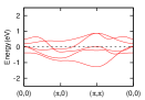
Figure 3: (Color online) (a) Original band structure and (b) renormalized band structure in the tetragonal phase. The dashed lines represent the chemical potentials.

(a)                            (b)

Figure 4: FSs for the (a) original and (b) renormalized band structures in the tetragonal phase.

(a)                                (b)

Figure 5: (Color online) DOSs for the (a) original and (b) renormalized band structures in the tetragonal phase. The dashed lines represent the chemical potentials.

(a)                       (b)

Figure 6: (Color online) (a) FS and (b) DOS for $\Delta_{\textrm{ortho.}}=0.08$. The dashed line represents the chemical potential.

As described in §2.1, a renormalized band structure is constructed in order to take into account the relatively strong electron correlation for the $d_{xz}$ and $d_{yz}$ orbitals. By this procedure, $(n_{\textrm{e}})_{xz+yz}$ becomes larger than that in the original band structure and is equal to 2.62, which is close to 3 (Table 1).

The obtained band structure, the corresponding FSs, and the density of states (DOS) in the tetragonal phase are shown in Figs. 3-5, respectively. For comparison, the original band structure, the corresponding FSs, and the DOS are also depicted in the figures.

Similarly, we calculate the FSs and DOS in the orthorhombic phase. As a typical case, the results for $\Delta_{\textrm{ortho.}}=0.08$ are shown in Fig. 6. The main effects of orthorhombic distortion are i) the disappearance of one of the FSs around the $\Gamma$-point [i.e., $\bm{k}=(0,0)$], and ii) the reduction of the DOS in the vicinity of the Fermi level.

3.2 Eigenvalue of the linearized gap equation

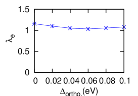
Figure 7: (Color online) Eigenvalue of the linearized gap equation, $\lambda_{\textrm{e}}$, for $0\leq\Delta_{\textrm{ortho.}}\leq 0.1$.

(a)                                (b)

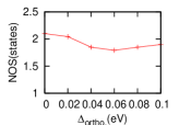
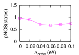
Figure 8: (Color online) (a) NOS and (b) pNOS for $d_{xz}$ and $d_{yz}$ orbitals in the vicinity of the Fermi level as a function of $\Delta_{\textrm{ortho.}}$.

(a)                            (b)

Figure 9: FSs for $\Delta_{\textrm{ortho.}}=$ (a) 0.02, and (b) 0.04. The main changes in the FSs are shown by arrows.

(a)                                   (b)

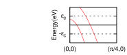
Figure 10: (Color online) Band structures around the $\Gamma$ point for $\Delta_{\textrm{ortho.}}=$ (a) 0.02, and (b) 0.04. Solid lines and dashed lines correspond to the chemical potentials and cutoff energies $\varepsilon_{\textrm{c}}$($=0.01$), respectively.

We investigate the eigenvalue, $\lambda_{\textrm{e}}$, of the linearized gap equation, eq. (16), for $0\leq\Delta_{\textrm{ortho.}}\leq 0.1$. Figure 7 shows the obtained eigenvalue, $\lambda_{\textrm{e}}$, as a function of $\Delta_{\textrm{ortho.}}$. We find that $\lambda_{\textrm{e}}$ decreases as $\Delta_{\textrm{ortho.}}$ increases. This result means that $T_{\textrm{c}}$ is highest in the tetragonal phase. In order to investigate the physical origin of this behavior of $\lambda_{\textrm{e}}$, we calculate the number of states (NOS) near the Fermi level, which is defined as the DOS integrated from $-\varepsilon_{\textrm{c}}$ to $\varepsilon_{\textrm{c}}$. Figure 8 shows the total NOS and the partial number of states (pNOS) for the $d_{xz}$ and $d_{yz}$ orbitals. Comparing Fig. 7 with Fig. 8, we consider that the physical origin of the behavior of $\lambda_{\textrm{e}}$ is the variation of the pDOS for the $d_{xz}$ and $d_{yz}$ orbitals. This result indicates that energy-splitting due to the orthorhombic distortion plays an important role in controlling $T_{\textrm{c}}$. A similar conclusion was also obtained theoretically for CeCoIn₅. [74]

Figure 7 also shows that $\lambda_{\textrm{e}}$ decreases with increasing $\Delta_{\textrm{ortho.}}$ for small values of $\Delta_{\textrm{ortho.}}$, while it does not change greatly for $\Delta_{\textrm{ortho.}}>0.05$. We speculate that this difference originates from the existence of a small hole pocket around the $\Gamma$-point. Figures 9 and 10 show the main changes in the FSs for $\Delta_{\textrm{ortho.}}=0.02$ and $0.04$ and the corresponding band structures near the $\Gamma$-point, respectively. The arrows in Fig. 9 represent the changes in the FSs. One of the small hole pockets around the $\Gamma$-point seems to disappear near $\Delta_{\textrm{ortho.}}=0.04$. We consider that the small hole pocket enhances $\lambda_{\textrm{e}}$. When it vanishes above $\Delta_{\textrm{ortho.}}=0.04$, $\lambda_{\textrm{e}}$ does not change further. A similar effect has been observed in a previous study for a system with multiple FSs. [75]

3.3 SC gap function and pairing symmetry

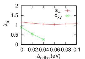
Figure 11: (Color online) Eigenvalue of the linearized gap equation $\lambda_{\textrm{e}}$ with $s$-wave and $d$-wave symmetries for $0\leq\Delta_{\textrm{ortho.}}\leq 0.1$.

(a) $\Delta_{11}$                            (b) $\Delta_{22}$

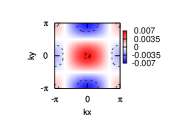
Figure 12: (Color online) SC gap functions $\Delta_{11}$ and $\Delta_{22}$ for $\Delta_{\textrm{ortho.}}=0$. The dashed lines represent the FSs for $\Delta_{\textrm{ortho.}}=0$.

(a) $\Delta_{11}$                            (b) $\Delta_{22}$

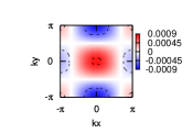
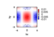
Figure 13: (Color online) SC gap functions $\Delta_{11}$ and $\Delta_{22}$ for $\Delta_{\textrm{ortho.}}=0.04$. The dashed lines represent the FSs for $\Delta_{\textrm{ortho.}}=0.04$.

$\Delta_{11/22}$

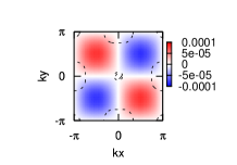
Figure 14: (Color online) SC gap functions $\Delta_{11/22}$ for a $d_{xy}$-wave pairing at $\Delta_{\textrm{ortho.}}=0$. The dashed lines represent the FSs for $\Delta_{\textrm{ortho.}}=0$.

(a)                                 (b)

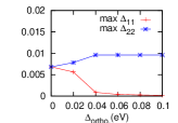
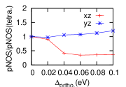
Figure 15: (Color online) (a) Maximum values of orbital-diagonal SC gap functions for $s_{+-}$-wave symmetry, max $\Delta_{11}$ and max $\Delta_{22}$, as a function of $\Delta_{\textrm{ortho.}}$ and (b) pNOSs for the $d_{xz}$ and $d_{yz}$ orbitals normalized by those in the tetragonal phase.

We now turn to the SC gap function and its pairing symmetry. Before we show the results of numerical calculations, we remark on the method used to determine the pairing symmetry for the multiorbital SC state within the linearized gap equation. [74] For the multiorbital SC state, there are two components of the SC gap function: orbital-diagonal and orbital-off-diagonal components. The pairing symmetry is determined from the orbital-diagonal SC gap function since it belongs to the same irreducible representation of the SC state. Hereafter, we show only the orbital-diagonal SC gap functions.

First, we investigate the most dominant pairing symmetry. As shown in Fig. 11, an unconventional fully gapped $s_{+-}$-wave pairing is the most stable for $0\leq\Delta_{\textrm{ortho.}}\leq 0.1$. As typical forms of the SC gap functions, $\Delta_{11}$ and $\Delta_{22}$ in the tetragonal and orthorhombic phases are shown in Figs. 12 and 13, respectively. At $\Delta_{\textrm{ortho.}}=0$, the second most stable pairing symmetry is a $d_{xy}$-wave pairing whose form is depicted in Fig. 14. Note that the values of $\lambda_{\textrm{e}}$ for other $d$-wave pairings (e.g., the $d_{x^{2}-y^{2}}$-wave pairing) are smaller than that for the $d_{xy}$-wave pairing.

Let us discuss the condition required to stabilize the $d_{xy}$-wave pairing. At $\Delta_{\textrm{ortho.}}=0$, the FS around the X- or Y-point [i.e., $(\pi,0)$ or $(0,\pi)$] does not have components of the $d_{xz}$ and $d_{yz}$ orbitals along the $k_{x}$- or $k_{y}$-direction, respectively. [75] Therefore, the energy cost is small even if a line node appears along the $k_{x}$- and $k_{y}$-axes. This is why the $d_{xy}$-wave pairing is stabilized. However, the rapid drop in $\lambda_{\textrm{e}}$ for the $d_{xy}$-wave pairing shown in Fig. 11 may be due to a subtle balance of the FSs around the $\Gamma$-point.

Finally, we investigate the anisotropy of the SC gap function in the orthorhombic phase. Figure 15(a) shows the maximum values of the SC gap functions, $\Delta_{11}$ and $\Delta_{22}$, as a function of $\Delta_{\textrm{ortho.}}$. When $\Delta_{\textrm{ortho.}}$ is on the order of 10$\%$ of the renormalized bandwidth ($\Delta_{\textrm{ortho.}}=$0.1), the ratio of max$\Delta_{11}$ to max$\Delta_{22}$ becomes 1$:$1000. Large anisotropy is thus expected for the SC state in the orthorhombic phase. With increasing $\Delta_{\textrm{ortho.}}$, the amplitude of $\Delta_{11}$ decreases rapidly, while that of $\Delta_{22}$ increases. [The SC gap functions for the $s_{+-}$-wave pairing become maximum at $\bm{k}=(0,0)$.] This behavior can be understood from the pNOS for the $d_{xz}$ and $d_{yz}$ orbitals shown in Fig. 15(b). We can see that $\Delta_{\textrm{ortho.}}$ markedly affects the pNOS for the $d_{xz}$ orbital, while it does not greatly affect that for the $d_{yz}$ orbital. This is because the energy level of the $d_{xz}$ orbital decreases to below the Fermi level. This variation of pNOSs leads to the decrease in $\Delta_{11}$ and increase of $\Delta_{22}$ as $\Delta_{\textrm{ortho.}}$ increases.

Since the experimentally observed SC gap function is the sum of the orbital-diagonal and orbital-off-diagonal components, the SC gap function becomes anisotropic in the case of different values of $\Delta_{11}$ and $\Delta_{22}$. Figure 15 indicates that the SC gap function around the X-point becomes larger than that around the Y-point for the SC state in the orthorhombic phase, since $\Delta_{22}$ is dominant in the orthorhombic phase and has this anisotropy (Fig. 13). We thus expect a large anisotropy of the SC gap function in the orthorhombic phase, which can be detected by ARPES measurement of the SC state in the orthorhombic phase. As we shall discuss in §4, this anisotropy is also expected in a SC state coexisting with a nematic state.

4 Discussion

First, we discuss the validity of neglecting the anisotropy of hopping integrals due to the orthorhombic distortion. According to a recent tight-binding calculation for the parent compound of LaFeAsO, [68] there is little significant difference in the hopping integrals for the $d_{xz}$ and $d_{yz}$ orbitals. Since we focus only on the region where the orthorhombic distortion is small ($\Delta_{\textrm{ortho.}}\leq 0.1$), the effect of the anisotropy on the hopping integrals is negligible. In other words, the effect of orthorhombic distortion on the energy-splitting will be more important than that on the hopping integrals in the presence of a small orthorhombic distortion. It is reasonable to consider only a small orthorhombic distortion since we consider the superconductivity in the doped case where the effect of orthorhombic distortion is suppressed.

We address the role of the spin-orbital coupling in determining the SC state. As shown in §2, the degeneracy of orbitals gives additional degrees of freedom which enhance the number of attractive channels for Cooper pairing. On the other hand, the orbital degree of freedom also has a depairing effect on superconductivity. In the present MFA, we have not clarified the depairing effect.

In iron-based compounds, As ions are located asymmetrically with respect to the Fe plane. [2] Therefore, there are many hopping integrals between Fe $3d$ orbitals, which are not allowed without As ions. This increases the number of interactions in eq. (9), which eventually increases the number of SC attractive channels. Note that these terms also enhance the magnetic instability; thus, they do not always favor the SC state.

Next, we compare our theory with other previous theoretical studies. As shown in §1, there are two different candidates for the pairing symmetry of the iron-based superconductors, i.e., $s_{+-}$-pairing [36, 37, 76, 77, 78, 79, 80, 81] and $s_{++}$-pairing [42, 43]. Our theory suggests the former pairing symmetry. Although the mechanism is not clear yet, we consider that the antiferromagnetism is closely related to the emergence of the superconductivity. Note that the quantum critical point of the antiferromagnetism has been observed for optimally doped $\textrm{Ba}\textrm{Fe}_{2}(\textrm{As}_{1-x}\textrm{P}_{x})_{2}$ by a nuclear magnetic resonance (NMR) measurement. [82] This result indicates that the antiferromagnetism plays an important role in the emergence of superconductivity for iron-based compounds.

We remark on the main difference between our theory and spin-fluctuation-mediated pairing, whether the glue of the superconductivity exists or not. In this paper, the SC attractive force originates directly from the KK-type superexchange interactions, while in spin-fluctuation theory, it originates from the fluctuation using a wide range of frequency space. Our obtained results have only n.n. and n.n.n. SC gap functions. This is qualitatively consistent with the SC gap functions obtained in the spin-fluctuation-mediated pairing, since the latter can be reproduced by the n.n. and n.n.n. parameters in real space. [83] The SC gap function observed in several ARPES measurements can also be fitted with the n.n. and n.n.n. parameters in real space. [10, 84] Therefore, the behaviors of $\lambda_{\textrm{e}}$ and the anisotropy between $\Delta_{11}$ and $\Delta_{22}$ as a function of $\Delta_{\textrm{ortho.}}$ will be qualitatively general in iron-based superconductors.

Next, we discuss the experimental correspondence for our assumption that the attractive interaction appears only among the special orbitals such as $d_{xz}$ and $d_{yz}$. This assumption is based on the idea that the AF state in parent compounds can be described by two localized orbitals. [52] Then, electrons in these orbitals induce superconductivity due to chemical doping and/or physical doping. We consider that this orbital-selective AF state does not contradict the experimental results for the metallic behavior, since the other orbitals have itinerant character. (A similar situation is expected in $\textrm{Ca}_{2-x}\textrm{Sr}_{x}\textrm{Ru}\textrm{O}_{4}$. [85]) As shown in §1, there are several experimental results that support our assumption: the large incoherence of the electronic Raman spectrum for these orbitals, [46] and the smaller mobility of holes observed in Hall resistivity measurement using a two-carrier model [47]. Note that the hole mobility will mainly originate from the $d_{xz}$ and $d_{yz}$ orbitals, since the hole pockets of the FS usually consists of these orbitals. Moreover, theoretical calculations for FeSe using the dynamical mean field theory [86, 87] show that the renormalization factors for the $d_{xz}$ and $d_{yz}$ orbitals are small ($=0.28$) compared with those of $d_{z^{2}}$ and $d_{x^{2}-y^{2}}$. (Note, however, that the renormalization factor for the $d_{xy}$ orbital is also small.) This is consistent with our assumption.

In $\textrm{Ba}_{1-x}\textrm{K}_{x}\textrm{Fe}_{2}\textrm{As}_{2}$ and $\textrm{Ba}\textrm{Fe}_{2}(\textrm{As}_{1-x}\textrm{P}_{x})_{2}$, however, the ARPES measurement [88] indicates that the $d_{z^{2}}$ orbital contributes to the FS, and the SC gap of the $d_{z^{2}}$ orbital is as large as that of the other orbitals. In this case, it is necessary to include the $d_{z^{2}}$ orbital, although the $d_{z^{2}}$ orbital can be a passive orbital for superconductivity.

We next address the possibility of superconductivity in the orthorhombic phase. Recently, the emergence of superconductivity in the orthorhombic phase with nearly 100$\%$ volume fraction has been reported for single crystals of $\textrm{Ba}_{0.6}\textrm{K}_{0.4}\textrm{Fe}_{2}\textrm{As}_{2}$, [3] although there have been some reports for the same compound that claim the inhomogeneous coexistence of SC and AF states. [26, 89] According to ref. 3, $T_{\textrm{c}}$ increases as the orthorhombicity $\delta=(a-b)/(a+b)$ decreases. This is consistent with our results. As discussed in §3.2, the decrease in $T_{\textrm{c}}$ due to the small orthorhombic distortion can be understood as the reduction of the pDOS for the $d_{xz}$ and $d_{yz}$ orbitals. Furthermore, in FeSe_0.94 under high pressure, the microscopic coexistence of SC and AF states in the region of higher pressure was observed by the muon-spin rotation measurement. [4] The SC state may also exist in the orthorhombic phase of $\textrm{Ba}(\textrm{Fe}_{1-x}\textrm{Co}_{x})_{2}\textrm{As}_{2}$. [33, 90]

On the other hand, in SrFe₂As₂ under high pressure, the NMR spectrum for the SC-dominant phase is almost equal to that for the tetragonal paramagnetic state. [18] This indicates that superconductivity is not realized in the orthorhombic phase. Although more detailed analysis in the presence of the AF order is needed, we consider that our effective model can qualitatively describe the properties of the SC state if superconductivity is realized in the orthorhombic phase.

Finally, we remark on the nematic state observed in the 122 system [44, 45], since the SC state coexisting with the nematic state is nearly the same as that in the orthorhombic phase. The nematic state is characterized by the lowering of rotational symmetry without any changes in the crystal structure. There have been some proposals of the emergence of the nematic state in strongly correlated systems such as cuprate [91] and Sr₃Ru₂O₇ [92]. In the iron-based compounds, its emergence has been proposed on the basis of experimental results for $\textrm{Ba}(\textrm{Fe}_{1-x}\textrm{Co}_{x})_{2}\textrm{As}_{2}$ [44, 45] and proposed theoretically. [93, 94, 95, 96] Although the effect of nematicity on the SC state has not been clarified, we propose that the anisotropy of the SC gap function, which is similar to that shown in Fig. 15(a), i.e., a difference between the SC gap functions around the X- and Y-points, can be observed if the SC state coexists with the nematic state.

5 Summary

We investigated the eigenvalue, $\lambda_{\textrm{e}}$, of the linearized gap equation and the pairing symmetry in a model for iron-based superconductors in both tetragonal and orthorhombic phases on the basis of the MFA. Our effective model consists of the five-orbital kinetic energy, the orthorhombic CEF energy, and the two-orbital KK-type superexchange interaction [64]. The effect of orthorhombic distortion on electronic states was taken into consideration as the energy-splitting of $d_{xz}$ and $d_{yz}$ orbitals, $\Delta_{\textrm{ortho.}}$. In order to take account of the relatively strong electron correlation, the procedure of band renormalization was used. We found a decrease in $\lambda_{\textrm{e}}$ accompanied with a reduction of the pNOS of the $d_{xz}$ and $d_{yz}$ orbitals near the Fermi level as $\Delta_{\textrm{ortho.}}$ increases. This result is consistent with the results of a recent experiment. [3] The fully gapped $s_{+-}$-wave symmetry pairing is predominant in both tetragonal and orthorhombic phases. $\lambda_{\textrm{e}}$ for the $d_{xy}$-wave pairing, which is the second most dominant symmetry, rapidly decreases as $\Delta_{\textrm{ortho.}}$ increases. The highest $T_{\textrm{c}}$ for the fully gapped $s_{+-}$-wave pairing is obtained in the tetragonal phase. The SC gap function for the fully gapped $s_{+-}$-wave pairing becomes anisotropic in the orthorhombic phase due to the crystal symmetry. We found large anisotropy of the SC gap function in the orthorhombic phase, $\textrm{max}\Delta_{11}$:$\textrm{max}\Delta_{22}\sim$1:1000, although $\Delta_{\textrm{ortho.}}$ is on the order on 10$\%$ of the renormalized bandwidth. Anisotropy originating from the difference in the values of the dominant orbital-diagonal SC gap function (i.e., $\Delta_{22}$) around the X- and Y-points can be detected by ARPES measurement if the superconductivity appears in the orthorhombic phase or in the coexisting phase with the nematic state.

We propose that the CEF energy plays an important role in controlling $T_{\textrm{c}}$ and the SC gap function for multiorbital superconductors, and consider that the orbital-selective superconductivity discussed in this paper will be universal for the structure-sensitive superconductivity observed in multiorbital systems.

- [1] Y. Kamihara, T. Watanabe, M. Hirano, and H. Hosono: J. Am. Chem. Soc. 130 (2008) 3296.
- [2] For a review on experiments, see K. Ishida, Y. Nakai, and H. Hosono: J. Phys. Soc. Jpn. 78 (2009) 062001; Y. Mizuguchi and Y. Takano: J. Phys. Soc. Jpn. 79 (2010) 102001.
- [3] D. Johrendt: 23rd International Symposium on Superconductivity, 2010, PC-5-INV.
- [4] M. Bendele, A. Amato, K. Conder, M. Elender, H. Keller, H.-H. Klauss, H. Luetkens, E. Pomjakushina, A. Raselli, and R. Khasanov: Phys. Rev. Lett. 104 (2010) 087003.
- [5] C.-H. Lee, A. Iyo, H. Eisaki, H. Kito, M. T. F. Diaz, T. Ito, K. Kihou, H. Matsuhata, M. Braden, and K. Yamada: J. Phys. Soc. Jpn. 77 (2008) 083704.
- [6] H. Yamashita, H. Mukuda, M. Yashima, S. Furukawa, Y. Kitaoka, K. Miyazawa, P. M. Shirage, H. Eisaki, and A. Iyo: J. Phys. Soc. Jpn. 79 (2010) 103703.
- [7] A. I. Coldea, J. D. Fletcher, A. Carrington, J. G. Analytis, A. F. Bangura, J. -H. Chu, A. S. Erickson, I. R. Fisher, N. E. Hussey, and R. D. McDonald: Phys. Rev. Lett. 101 (2008) 216402.
- [8] A. I. Coldea, C. M. J. Andrew, J. G. Analytis, R. D. McDonald, A. F. Bangura, J.-H. Chu, I. R. Fisher, and A. Carrington: Phys. Rev. Lett. 103 (2009) 026404.
- [9] H. Shishido, A. F. Bangura, A. I. Coldea, S. Tonegawa, K. Hashimoto, S. Kasahara, P. M. C. Rourke, H. Ikeda, T. Terashima, R. Settai, Y. nuki, D. Vignolles, C. Proust, B. Vignolle, A. McCollam, Y. Matsuda, T. Shibauchi, and A. Carrington: Phys. Rev. Lett. 104 (2010) 057008.
- [10] K. Nakayama, T. Sato, P. Richard, Y.-M. Xu, Y. Sekiba, S. Souma, G. F. Chen, J. L. Luo, N. L. Wang, H. Ding, and T. Takahashi: Europhys. Lett. 85 (2009) 67002.
- [11] A. Tamai, A. Y. Ganin, E. Rozbicki, J. Bacsa, W. Meevasana, P. D. C. King, M. Caffio, R. Schaub, S. Margadonna, K. Prassides, M. J. Rosseinsky, and F. Baumberger: Phys. Rev. Lett. 104 (2010) 097002.
- [12] Q. Huang, Y. Qiu, W. Bao, M. A. Green, J. W. Lynn, Y. C. Gasparovic, T. Wu, G. Wu, and X. H. Chen: Phys. Rev. Lett. 101 (2008) 257003.
- [13] A. Jesche, C. Krellner, M. de Souza, M. Lang, and C. Geibel: Phys. Rev. B 81 (2010) 134525.
- [14] S. Li, C. de la Cruz, Q. Huang, Y. Chen, J. W. Lynn, J. Hu, Y.-L. Huang, F.-C. Hsu, K.-W. Yeh, M.-K. Wu, and P. Dai: Phys. Rev. B 79 (2009) 054503.
- [15] C. de la Cruz, Q. Huang, J. W. Lynn, J. Li, W. Ratcliff, II, J. L. Zarestky, H. A. Mook, G. F. Chen, J. L. Luo, N. L. Wang, and P. Dai: Nature 453 (2008) 899.
- [16] W. Tian, W. Ratcliff, II, M. G. Kim, J.-Q. Yan, P. A. Kienzle, Q. Huang, B. Jensen, K. W. Dennis, R. W. McCallum, T. A. Lograsso, R. J. McQueeney, A. I. Goldman, J. W. Lynn, and A. Kreyssig: Phys. Rev. B 82 (2010) 060514 (R).
- [17] K. Kitagawa, N. Katayama, K. Ohgushi, M. Yoshida, and M. Takigawa: J. Phys. Soc. Jpn. 77 (2008) 114709.
- [18] K. Kitagawa, N. Katayama, H. Gotou, T. Yagi, K. Ohgushi, T. Matsumoto, Y. Uwatoko, and M. Takigawa: Phys. Rev. Lett. 103 (2009) 257002.
- [19] H.-J. Grafe, D. Paar, G. Lang, N. J. Curro, G. Behr, J. Werner, J. Hamann-Borrero, C. Hess, N. Leps, R. Klingeler, and B. Bchner: Phys. Rev. Lett. 101 (2008) 047003.
- [20] K. Matano, Z. A. Ren, X. L. Dong, L. L. Sun, Z. X. Zhao, and G.-Q. Zheng: Europhys. Lett. 83 (2008) 57001.
- [21] M. Yashima, H. Nishimura, H. Mukuda, Y. Kitaoka, K. Miyazawa, P. M. Shirage, K. Kihou, H. Kito, H. Eisaki, and A. Iyo: J. Phys. Soc. Jpn. 78 (2009) 103702.
- [22] Z. Li, Y. Ooe, X.-C. Wang, Q.-Q. Liu, C.-Q. Jin, M. Ichioka, and G.-Q. Zheng: J. Phys. Soc. Jpn. 79 (2010) 083702.
- [23] Y. Nakai, K. Ishida, Y. Kamihara, M. Hirano, and H. Hosono: J. Phys. Soc. Jpn. 77 (2008) 073701.
- [24] Y. Kobayashi, A. Kawabata, S. C. Lee, T. Moyoshi, and M. Sato: J. Phys. Soc. Jpn. 78 (2009) 073704.
- [25] F. Hammerath, S.-L. Drechsler, H.-J. Grafe, G. Lang, G. Fuchs, G. Behr, I. Eremin, M. M. Korshunov, and B. Bchner: Phys. Rev. B 81 (2010) 140504 (R).
- [26] H. Fukazawa, T. Yamazaki, K. Kondo, Y. Kohori, N. Takeshita, P. M. Shirage, K. Kihou, K. Miyazawa, H. Kito, H. Eisaki, and A. Iyo: J. Phys. Soc. Jpn. 78 (2009) 033704.
- [27] F. Ning, K. Ahilan, T. Imai, A. S. Sefat, R. Jin, M. A. McGuire, B. C. Sales, and D. Mandrus: J. Phys. Soc. Jpn. 77 (2008) 013711.
- [28] Y. Nakai, T. Iye, S. Kitagawa, K. Ishida, S. Kasahara, T. Shibauchi, Y. Matsuda, and T. Terashima: Phys. Rev. B 81 (2010) 020503 (R).
- [29] S. Masaki, H. Kotegawa, Y. Hara, H. Tou, K. Murata, Y. Mizuguchi, and Y. Takano: J. Phys. Soc. Jpn. 78 (2009) 063704.
- [30] M. Sato, Y. Kobayashi, S. C. Lee, H. Takahashi, E. Satomi, and Y. Miura: J. Phys. Soc. Jpn. 79 (2010) 014710.
- [31] S. C. Lee, E. Satomi, Y. Kobayashi, and M. Sato: J. Phys. Soc. Jpn. 79 (2010) 023702.
- [32] P. Cheng, B. Shen, J. Hu, and H.-H. Wen: Phys. Rev. B 81 (2010) 174529.
- [33] S. Nandi, M. G. Kim, A. Kreyssig, R. M. Fernandes, D. K. Pratt, A. Thaler, N. Ni, S. L. Bud’ko, P. C. Canfield, J. Schmalian, R. J. McQueeney, and A. I. Goldman: Phys. Rev. Lett. 104 (2010) 057006.
- [34] M. G. Kim, D. K. Pratt, G. E. Rustan, W. Tian, J. L. Zarestky, A. Thaler, S. L. Bud’ko, P. C. Canfield, R. J. McQueeney, A. Kreyssig, and A. I. Goldman: Phys. Rev. B 83 (2011) 054514.
- [35] N. Katayama, S. Ji, D. Louca, S. Lee, M. Fujita, T. J. Sato, J. Wen, Z. Xu, G. Gu, G. Xu, Z. Lin, M. Enoki, S. Chang, K. Yamada, and J. M. Tranquada: J. Phys. Soc. Jpn. 79 (2010) 113702.
- [36] I. I. Mazin, D. J. Singh, M. D. Johannes, and M. H. Du: Phys. Rev. Lett. 101 (2008) 057003.
- [37] K. Kuroki, S. Onari, R. Arita, H. Usui, Y. Tanaka, H. Kontani, and H. Aoki: Phys. Rev. Lett. 101 (2008) 087004.
- [38] A. D. Christianson, E. A. Goremychkin, R. Osborn, S. Rosenkranz, M. D. Lumsden, C. D. Malliakas, I. S. Todorov, H. Claus, D. Y. Chung, M. G. Kanatzidis, R. I. Bewley, and T. Guidi: Nature 456 (2008) 930.
- [39] H. Mukuda, M. Nitta, M. Yashima, Y. Kitaoka, P. M. Shirage, H. Eisaki, and A. Iyo: J. Phys. Soc. Jpn. 79 (2010) 113701.
- [40] T. Hanaguri, S. Niitaka, K. Kuroki, and H. Takagi: Science 328 (2010) 1187399.
- [41] Y. Senga and H. Kontani: J. Phys. Soc. Jpn. 77 (2008) 113710; S. Onari and H. Kontani: Phys. Rev. Lett. 103 (2009) 177001.
- [42] H. Kontani and S. Onari: Phys. Rev. Lett. 104 (2010) 157001; T. Saito, S. Onari, and H. Kontani: Phys. Rev. B 82 (2010) 144510; S. Onari and H. Kontani: arXiv: 1009.3882.
- [43] Y. Yanagi, Y. Yamakawa, N. Adachi, and Y. no: Phys. Rev. B. 82 (2010) 065418; Y. Yanagi, Y. Yamakawa, N. Adachi, and Y. no: J. Phys. Soc. Jpn. 79 (2010) 123707.
- [44] J.-H. Chu, J. G. Analytis, K. D. Greve, P. L. McMahon, Z. Islam, Y. Yamamoto, and I. R. Fisher: Science 329 (2010) 824.
- [45] M. Yi, D. H. Lu, J.-H. Chu, J. G. Analytis, A. P. Sorini, A. F. Kemper, S.-K. Mo, R. G. Moore, M. Hashimoto, W. S. Lee, Z. Hussain, T. P. Devereaux, I. R. Fisher, and Z.-X. Shen: Proc. Natl. Acad. Sci. U. S. A. 108 (2011) 6878.
- [46] B. Muschler, W. Prestel, R. Hackl, T. P. Devereaux, J. G. Analytis, J.-H. Chu, and I. R. Fisher: Phys. Rev. B 80 (2009) 180510 (R).
- [47] F. R. Albenque, D. Colson, A. Forget, and H. Alloul: Phys. Rev. Lett. 103 (2009) 057001.
- [48] T. Shimojima, K. Ishizaka, Y. Ishida, N. Katayama, K. Ohgushi, T. Kiss, M. Okawa, T. Togashi, X.-Y. Wang, C.-T. Chen, S. Watanabe, R. Kadota, T. Oguchi, A. Chainani, and S. Shin: Phys. Rev. Lett. 104 (2010) 057002.
- [49] R. M. Fernandes, L. H. VanBebber, S. Bhattacharya, P. Chandra, V. Keppens, D. Mandrus, M. A. McGuire, B. C. Sales, A. S. Sefat, and J. Schmalian: Phys. Rev. Lett. 105 (2010) 157003.
- [50] M. Yoshizawa, R. Kamiya, R. Onodera, Y. Nakanishi, K. Kihou, H. Eisaki, A. Iyo, and C. H. Lee: arXiv: 1008.1479.
- [51] A. Kreyssig, M. G. Kim, S. Nandi, D. K. Pratt, W. Tian, J. L. Zarestky, N. Ni, A. Thaler, S. L. Bud’ko, P. C. Canfield, R. J. McQueeney, and A. I. Goldman: Phys. Rev. B 81 (2010) 134512.
- [52] C.-C. Lee, W.-G. Yin, and W. Ku: Phys. Rev. Lett. 103 (2009) 267001.
- [53] K. Kubo and P. Thalmeier: J. Phys. Soc. Jpn. 78 (2009) 083704.
- [54] K. Kubo and P. Thalmeier: arXiv: 1010.4626.
- [55] T. Terashima, M. Kimata, N. Kurita, H. Satsukawa, A. Harada, K. Hazama, M. Imai, A. Satao, K. Kihou, C.-H. Lee, H. Kito, H. Eisaki, A. Iyo, T. Saito, H. Fukazawa, Y. Kohori, H. Harima, and S. Uji: J. Phys. Soc. Jpn. 79 (2010) 053702.
- [56] M. Yi, D. H. Lu, J. G. Analytis, J.-H. Chu, S.-K. Mo, R.-H. He, R. G. Moore, X. J. Zhou, G. F. Chen, J. L. Luo, N. L. Wang, Z. Hussain, D. J. Singh, I. R. Fisher, and Z.-X. Shen: Phys. Rev. B 80 (2009) 024515.
- [57] J. G. Analytis, C. M. J. Andrew, A. I. Coldea, A. McCollam, J.-H. Chu, R. D. McDonald, I. R. Fisher, and A. Carrington: Phys. Rev. Lett. 103 (2009) 076401.
- [58] A. Yamasaki, Y. Matsui, S. Imada, K. Takase, H. Azuma, T. Muro, Y. Kato, A. Higashiya, A. Sekiyama, S. Suga, M. Yabashi, K. Tamasaku, T. Ishikawa, K. Terashima, H. Kobori, A. Sugimura, N. Umeyama, H. Sato, Y. Hara, N. Miyakawa, and S. I. Ikeda: Phys. Rev. B 82 (2010) 184511.
- [59] R. Yoshida, T. Wakita, H. Okazaki, Y. Mizuguchi, S. Tsuda, Y. Takano, H. Takeya, K. Hirata, T. Muro, M. Okawa, K. Ishizaka, S. Shin, H. Harima, M. Hirai, Y. Muraoka, and T. Yokoya: J. Phys. Soc. Jpn. 78 (2009) 034708.
- [60] A. Lucarelli, A. Dusza, F. Pfuner, P. Lerch, J. G. Analytis, J.-H. Chu, I. R. Fisher, and L. Degiorgi: New J. Phys. 12 (2010) 073036.
- [61] F. Krger, S. Kumar, J. Zaanen, and J. van der Brink: Phys. Rev. B 79 (2009) 054504.
- [62] W. Lv, J. Wu, and P. Phillips: Phys. Rev. B 80 (2009) 224506.
- [63] C.-C. Chen, J. Maciejko, A. P. Sorini, B. Moritz, R. R. P. Singh, and T. P. Devereaux: Phys. Rev. B 82 (2010) 100504 (R).
- [64] K. I. Kugel’ and D. I. Khomskiĭ: Sov. Phys. JETP 3 (1973) 4.
- [65] K. Seo, B. A. Bernevig, and J. Hu: Phys. Rev. Lett. 101 (2008) 206404.
- [66] M. C. Gutzwiller: Phys. Rev. Lett. 10 (1963) 159; M. C. Gutzwiller: Phys. Rev. 137 (1965) A1726.
- [67] M. M. Qazilbash, J. J. Hamlin, R. E. Baumbach, L. Zhang, D. J. Singh, M. B. Maple, and D. N. Basov: Nat. Phys. 5 (2009) 647.
- [68] Z. P. Yin and W. E. Pickett: Phys. Rev. B 81 (2010) 174534.
- [69] Q. Si and E. Abrahams: Phys. Rev. Lett. 101 (2008) 076401.
- [70] T. Yildirium: Phys. Rev. Lett. 101 (2008) 057010.
- [71] M. J. Han, Q. Yin, W. E. Pickett, and S. Y. Savrasov: Phys. Rev. Lett. 102 (2009) 107003.
- [72] E. Bascones, M. J. Caldern, and B. Valenzuela: Phys. Rev. Lett. 104 (2010) 227201.
- [73] S. Zhou and Z. Wang: Phys. Rev. Lett. 105 (2010) 096401.
- [74] T. Takimoto, T. Hotta, and K. Ueda: Phys. Rev. B 69 (2004) 104504.
- [75] K. Kuroki, H. Usui, S. Onari, R. Arita, and H. Aoki: Phys. Rev. B 79 (2009) 224511.
- [76] T. Nomura: J. Phys. Soc. Jpn. 78 (2008) 034716.
- [77] H. Ikeda: J. Phys. Soc. Jpn. 77 (2008) 123707; H. Ikeda, R. Arita, and J. Kune: Phys. Rev. B 81 (2010) 054502.
- [78] F. Wang, H. Zhai, Y. Ran, A. Vishwanath, and D.-H. Lee: Phys. Rev. Lett. 102 (2008) 047005.
- [79] Y. Fuseya, T. Kariyado, and M. Ogata: J. Phys. Soc. Jpn. 78 (2009) 023703.
- [80] S. Graser, A. F. Kemper, T. A. Maier, H.-P. Cheng, P. J. Hirschfeld, and D. J. Scalapino: Phys. Rev. B 81 (2010) 214503.
- [81] K. Suzuki, H. Usui, and K. Kuroki: J. Phys. Soc. Jpn. 80 (2011) 013710.
- [82] Y. Nakai, T. Iye, S. Kitagawa, K. Ishida, H. Ikeda, S. Kasahara, H. Shishido, T. Shibauchi, Y. Matsuda, and T. Terashima: Phys. Rev. Lett. 105 (2010) 107003.
- [83] T. Kariyado and M. Ogata: J. Phys. Soc. Jpn. 79 (2010) 033703; T. Kariyado and M. Ogata: J. Phys. Soc. Jpn. 79 (2010) 083704.
- [84] Y.-M. Xu, Y.-B. Huang, X.-Y. Cui, E. Razzoli, M. Radovic, M. Shi, G.-F. Chen, P. Zheng, N.-L. Wang, C.-L. Zhang, P.-C. Dai, J.-P. Hu, Z. Wang, and H. Ding: Nat. Phys. 7 (2011) 1.
- [85] A. Koga, N. Kawakami, T. M. Rice, and M. Sigrist: Phys. Rev. Lett. 92 (2004) 216402.
- [86] M. Aichhorn, S. Biermann, T. Miyake, A. Georges, and M. Imada: Phys. Rev. B 82 (2010) 064504.
- [87] L. Craco, M. S. Laad, and S. Leoni: arXiv: 0910.3828.
- [88] T. Shimojima (private communication).
- [89] J. T. Park, D. S. Inosov, Ch. Niedermayer, G. L. Sun, D. Haug, N. B. Christensen, R. Dinnebier, A. V. Boris, A. J. Drew, L. Schulz, T. Shapoval, U. Wolff, V. Neu, X. Yang, C. T. Lin, B. Keimer, and V. Hinkov: Phys. Rev. Lett. 102 (2009) 117006.
- [90] D. K. Pratt, W. Tian, A. Kreyssig, J. L. Zarestky, S. Nandi, N. Ni, S. L. Bud’ko, P. C. Canfield, A. I. Goldman, and R. J. McQueeney: Phys. Rev. Lett. 103 (2009) 087001.
- [91] Y. Ando, K. Segawa, S. Komiya, and A. N. Lavrov: Phys. Rev. Lett. 88 (2002) 137005.
- [92] R. A. Borzi, S. A. Grigera, J. Farrell, R. S. Perry, S. J. S. Lister, S. L. Lee, D. A. Tennant, Y. Maeno, and A. P. Mackenzie: Science 315 (2007) 1134796.
- [93] C. Fang, H. Yao, W.-F. Tsai, J. P. Hu, and S. A. Kivelson: Phys. Rev. B 77 (2008) 224509 (R).
- [94] W.-C. Lee and C. Wu: Phys. Rev. Lett. 103 (2009) 176101.
- [95] J. Knolle, I. Eremin, A. Akbari, and R. Moessner: Phys. Rev. Lett. 104 (2010) 257001.
- [96] S. A. J. Kimber, D. N. Argyriou, and I. I. Mazin: arXiv: 1005.1761.