The Origin of Planetary System Architectures. I. Multiple Planet Traps in Gaseous Discs

Abstract

The structure of planetary systems around their host stars depends on their initial formation conditions. Massive planets will likely be formed as a consequence of rapid migration of planetesimals and low mass cores into specific trapping sites in protoplanetary discs. We present analytical modeling of inhomogeneities in protoplanetary discs around a variety of young stars, - from Herbig Ae/Be to classical T Tauri and down to M stars, - and show how they give rise to planet traps. The positions of these traps define the initial orbital distribution of multiple protoplanets. We investigate both corotation and Lindblad torques, and show that a new trap arises from the (entropy-related) corotation torque. This arises at that disc radius where disc heating changes from viscous to stellar irradiation dominated processes. We demonstrate that up to three traps (heat transitions, ice lines and dead zones) can exist in a single disc, and that they move differently as the disc accretion rate $\dot{M}$ decreases with time. The interaction between the giant planets which grow in such traps may be a crucial ingredient for establishing planetary systems. We also demonstrate that the position of planet traps strongly depends on stellar masses and disc accretion rates. This indicates that host stars establish preferred scales of planetary systems formed around them. We discuss the potential of planet traps induced by ice lines of various molecules such as water and CO, and estimate the maximum and minimum mass of planets which undergo type I migration. We finally apply our analyses to accounting for the initial conditions proposed in the Nice model for the origin of our Solar system.

1 Introduction

Observations of exoplanets (nearly $\sim$ 1700 if candidates are included) show that the formation of multiple planets around their host stars is relatively common. This trend is confirmed by both the radial velocity and transit techniques such as the Kepler mission (e.g. Howard et al., 2011). Many previous studies based on N-body simulations, investigated the dynamics of the planetary systems (e.g. Rasio & Ford, 1996). It is well known that these simulations can reproduce the observed distribution of eccentricities of exoplanets very well, if they adopt a specific initial condition that planets are closely packed (e.g. Ford & Rasio, 2008). For our Solar system, the Nice model which requires a specific initial arrangement of Jupiter and Saturn explains the dynamics very well (Morbidelli, 2010, references herein). The obvious question is whether or not such conditions are reasonable. In order to answer the question, one needs to consider the early stage of planet formation in which physical processes are controlled by gas dynamics in discs (e.g. Thommes et al., 2008). The presence of gas is necessary for gas giants to be formed. However, it also causes rapid inward planetary migration (Ward, 1997). Since this radial motion strongly depends on the disc properties such as the gas surface density and the disc temperature, it becomes a huge challenge to systematically investigate what are the realistic initial conditions for the later evolution of planetary systems.

Recently, planet traps have received a lot of attention (Masset et al., 2006; Morbidelli et al., 2008). Barriers to planetary migration arise because of inhomogeneities in discs where the direction of planetary migration switches from inwards to outwards, so that migrating planets are halted. (Equivalently, the net torque exerted on planets is zero there, Hasegawa & Pudritz, 2010a, hereafter HP10, references herein). Planets may acquire most of their mass as they accrete material at these barriers - which we call planet traps in globally evolving discs. We use the term barriers for our local analyses ($\S$ 3 and 4) while the term of planet traps are used for our global, unified analyses ($\S$ 6).

Planet traps were originally proposed by Masset et al. (2006) in order to solve the well known rapid migration problem wherein planets can be lost to discs within $10^{5}$ years. Matsumura et al. (2007, hereafter MPT07) first addressed a (possible) link between the planet traps and the diversity of exoplanets by showing that planet traps can move due to the time dependent, viscous evolution of discs (also see Matsumura et al., 2009). Although they focused on dead zones in discs (which are the high density, inner regions, so that turbulence there induced by magnetorotational instability (MRI) is quenched, Gammie, 1996), their basic idea is valid for any type of planet trap. More recently, it has been pointed out that a single disc can have a couple of planet traps (Ida & Lin, 2008; Lyra et al., 2010). Population synthesis models confirm that the planet traps and their movements can be important for the diversity of observed exoplanetary systems (Mordasini et al., 2011). As already noted, planet traps have the possibility of strongly enhancing the growth rate of planetary cores (Sándor et al., 2011) and the formation of giant planets. Thus, planet traps have considerable potential for understanding the formation of planetary systems.

In a series of papers, we systematically investigate how inhomogeneities in discs can trap migrating planets in overdense regions where they undergo most of their growth, and how trapped planets establish their planetary systems in viscously evolving discs. In this paper, we undertake a comprehensive study of the various mechanisms that produce planet traps in discs around a variety of young stars, - from high to low mass. One of our major findings is that a single disc can have up to three planet trap regions. We show that the position of any trap depends upon the disc’s accretion rate, which decreases with time as the disc is used up and star formation is terminated. The decreasing accretion rate forces the planet traps to move inwards at varying rates. This ultimately sets up the condition for the mutual interaction of planets in the traps, which can provide the realistic initial conditions for the evolution of planetary systems.

The plan of this paper is as follows. We describe physical processes that create inhomogeneities in discs and summarise our analytical approach for them in $\S$ 2. The general reader may then proceed to $\S$ 6 for discussion of the general results (also see Fig. 7). Armed with physical understanding of the inhomogeneities, we investigate corotation and Lindblad torques which are the driving force of planetary migration in $\S$ 3 and 4, respectively. For the former case, we show that a new barrier arises due to the change of the main heat source for gas disc from viscosity to stellar irradiation. For both torques, ice lines play some role in trapping planets (Ida & Lin 2008, hereafter IL08; Lyra et al. 2010). In $\S$ 5, we discuss other possible barriers and estimate the maximum and minimum mass with which planets undergo type I migration. Also, we investigate the possibility of the presence of ice lines due to various molecules. In $\S$ 6, we integrate our analyses and discuss the roles of these planet traps in the formation of planetary systems. We apply our results to an explanation of the Nice model for the architecture of the Solar system in $\S$ 7. In $\S$ 8, we present our conclusions. We summarise important quantities which often appear in this paper in Table 1.

Table 1: Important quantities

Symbols	Meaning
$M_{*}$	Stellar mass
$R_{*}$	Stellar radius
$T_{*}$	Stellar effective temperature
$\dot{M}$	Accretion rate (see equation (3.6))
$G$	Gravitational constant
$\Omega$	Angular frequency (see equation (4.3))
$\Omega_{Kep}$	Keplerian frequency ($=\sqrt{GM_{*}/r^{3}}$)
$M_{p}$	Planetary mass
$r_{p}$	Planetary orbital radius
$\mu$	$M_{p}/M_{*}$
$\rho$	Gas volume density
$\Sigma^{1}$	Gas surface density
$\Sigma_{0}$	Gas surface density at $r=r_{0}$
$s^{1}$	Power-law index of $\Sigma$ if $\Sigma\propto r^{s}$
$T$	Disc temperature ($\propto r^{t}$)
$t$	Power-law index of $T$
$T_{e}$	Disc effective temperature
$T_{m}$	Disc temperature of the mid-plane
$T_{m,k}(r_{il})$	Condensation temperature for species $k$ at the ice line
$T_{s}$	Disc temperature of the surface
$c_{s}$	Sound speed ($\propto\sqrt{T}$)
$H$	Disc scale height ($=c_{s}/\Omega$)
$\bar{H}$	Disc photosphere height
$h$	Disc aspect ratio ($=H/r$)
$r_{trans}$	Disc radius of disc inhomogeneities
$F_{g}$	Gas density modification at $r_{trans}$
$\omega$	Transition width at $r_{trans}$ ($=cH$)
$r_{ht}$	Disc radius of the heat transition
$r_{il}$	Disc radius of ice lines
$r_{edge}$	Disc radius of the outer edge of dead zones
$p$	Gas pressure ($=\rho c_{s}^{2}$)
$\kappa$	Epicyclic frequency (see equation (4.4))
$m$	Wavenumber (see equation (4.2))
$\alpha_{r}$	Lindblad resonant position ($=r/r_{p}$)
$\psi$	Forcing function (see equations (4.5) and (4.12))
$X_{p}$	Value of a quantity $X$ at $r_{p}$
$\Sigma_{A}$	Surface density of active regions (see equation (4.24))
$s_{A}$	Power-law index of $\Sigma_{A}$ (generally $>0$)
$r_{0}$	Characteristic disc radius
$f_{ice}$	Modification factor of $\Sigma_{A}$ due to ice lines ($=f(r_{il},f_{d1},f_{d2})$)
$f_{d1}$	Parameter representing density jumps due to ice lines
$f_{d2}$	Parameter representing dust traps due to ice lines
$g_{d}$	Parameter representing density bumps due to ice lines
$\alpha$	Mean strength of turbulence (see equation (4.21))
$\alpha_{A}$	Strength of turbulence in the active zone ($=10^{-2}$)
$\alpha_{D}$	Strength of turbulence in the dead zone ($=10^{-5}$)
$\nu$	Kinematic viscosity ($=\alpha c_{s}H$)
$\gamma$	Adiabatic index (=1.4)
$F_{z}$	Heat flux in the vertical direction
$D_{vis}$	Viscous dissipation rate per unit mass
$\sigma_{SB}$	the Stefan-Boltzmann constant
$k_{B}$	the Boltzmann constant
$\alpha_{GA}$	Grazing angle (see equation (3.20))
$\bar{\kappa}$	Opacity
$\tau$	Optical depth ($=\bar{\kappa}\Sigma$)

¹ The simplest assumption that $\Sigma\propto r^{s}$ is only adopted in $\S$ 3.2 and 4.2.

2 Disc inhomogeneities

We describe physical processes governing the structure of protoplanetary discs and discuss how disc inhomogeneities arises from these processes. We discuss the basic features of our analytical modeling of the resultant disc structures - which will be presented in $\S$ 3 and 4. Table 2 summarises the disc inhomogeneities, related nomenclature that often appears in the literature, the dominant torque that transports angular momentum in that region of the disc, and the section of the paper that treats the analysis.

Table 2: Summary of disc inhomogeneities

Disc inhomogeneity	Nomenclature	Torque	Section
Opacity transitions	e.g. Ice lines1	Corotation	3.2.4
Heat transitions	N/A	Corotation	3.2.3
Turbulence transitions	Dead zones	Lindblad	4.3
Opacity and turbulent transitions	Ice lines2	Lindbald	4.4

¹ Disc turbulence is assumed to originate from non-MRI based processes

² Disc turbulence is assumed to originate from MRI based processes

2.1 Physical processes

Heating of protoplanetary discs is one of the most important processes in order to understand their geometrical structure (e.g. Dullemond et al., 2007). Since discs are accreted onto the central stars, release of gravitational energy through disc accretion becomes one of the main heat sources. This energy can be dissipated by viscous stresses, leading to viscous heating. Once discs are heated up, then the absorption efficiency of discs which is regulated by their optical depth establishes the thermal structure of discs. In protoplanetary discs, dust gives the main contribution to opacity for photons with low to intermediate energy while gas is the main absorber of high energy photons. In the inner region of discs, viscous heating is very efficient and leads to high disc temperatures ($\gtrsim$ 1000 K for classical T Tauri stars (CTTSs), D’Alessio et al., 1998). As a result, both metal dust grains and molecules are destroyed there (e.g. Bell & Lin, 1994). Thus, this high disc temperature and resultant destruction of opacity sources produces opacity transitions. It is interesting that opacity transitions are also produced in a completely different situation, that is, of low disc temperatures wherein opacity is enhanced by ”freeze-out” processes. Ice lines are one of the most famous opacity transitions created by this process. Ice lines are defined such that the number density of ice-coated dust grains suddenly increases, which is a consequence of low disc temperatures there. In $\S$ 3.2.4, we treat ice lines as an example of opacity transitions.

It is well known that protoplanetary discs are also heated up by stellar irradiation (Chiang & Goldreich, 1997; Hasegawa & Pudritz, 2010b). Since viscous heating becomes less efficient for larger disc radii, stellar irradiation plays a dominant role in regulating the thermal structure of discs there. Thus, a transition exists for discs wherein the dominant heating mechanism transits from viscous heating to stellar irradiation. We call this a heat transition. (see $\S$ 3.2.3).

We have focused so far on heating processes which involve with photons that have relatively low energy. High energy photons such as X-rays from the central stars and cosmic rays, are important for understanding the ionization of protoplanetary discs. Since the MRI is the most favoured process to excite turbulence in discs, it is crucial to evaluate the ionization structure of discs (Gammie, 1996). In the inner region of discs, the column density is very high, so that high energy photons cannot penetrate the entire region. In this ”layered” structure, the mid-plane is effectively screened from being ionized while the surface region is efficiently ionized. Thus, the inner region is less turbulent, and characterised by a dead zone. On the other hand, the outer region has lower column density and hence is fully ionized for the entire region including the mid-plane. As a result, the outer region is fully turbulent. Thus, transitions in the amplitude of turbulence exist in discs which we denote as turbulent transitions (see $\S$ 4.3). Dead zones are the most famous product of the turbulent transitions.

Finally, we introduce interesting transitions which arise from the combination of opacity and turbulent transitions. If the MRI is the mechanism that drives disc turbulence, then ice lines can also be regarded as this type of transition (IL08, see $\S$ 4.4.1 for the complete discussion). At the ice lines, the sudden increment of ice-coated dust grains is likely to result in the sudden decrement of free electrons there, since such sticky grains can efficiently absorb them (Sano et al., 2000). This process, initiated by the opacity transitions, reduces the ionization level there, and therefore removes the coupling between the magnetic field and the gas - which kills the MRI instability. Hence ice lines create turbulent transitions. In summary, ice lines are regarded as an opacity transition if disc turbulence is excited by non MRI processes while they act as an opacity and turbulent transition if turbulence is excited by the MRI. In $\S$ 4.4, we investigate ice lines again, but as an example of the opacity and turbulent transitions.

2.2 Our analytical approach

We present analytical modeling of the disc structures affected by the disc inhomogeneities in $\S$ 3 and 4. In order to make analytical treatments possible, we adopt expressions that are simple enough, but well capture the physics arising from the inhomogeneities. As an example, we adopt a $\tanh$ function for representing an inhomogeneity in the surface density (see equation (3.1)). This profile is more general than a power-law and is likely to be applicable for the cases of opacity, heat, and turbulent transitions. For the opacity and heat transitions, the results of Menou & Goodman (2004, hereafter MG04, see their fig1) validate the usage of this function as do the results of MPT07 for the turbulent transitions. Disc structures are approximated as power-laws for regions far away from the inhomogeneities (see equation (3.1)). Thus, we adopt more general profiles for the disc structures. In addition, we make use of the simplest expressions in order to reduce mathematical complexity, and hence different functions are adopted for different transitions.

Bearing these in mind, we will demonstrate that the disc inhomogeneities are the most plausible sites to produce barriers to type I migration by undertaking a comprehensive study of both corotation and Lindblad torques in $\S$ 3 and 4, respectively.

3 Barriers arising from corotation torques

Corotation torques play an important role in planetary migration in regions with high viscosity ($10^{-1}\lesssim\alpha\lesssim 10^{-3}$), because the corotation torque there is (partially) unsaturated (i.e. effective, see Appendix B in Hasegawa & Pudritz 2011, references herein). The corotation torque is known to act as a barrier for two situations. The first situation is when $\Sigma\propto r^{s}$ with $s\gtrsim 1$ (Masset et al., 2006; Paardekooper & Papaloizou, 2009). This case can be generally established only at the inner edge of discs. In typical discs, the inner edge is located around a few hundredths of au, which corresponds to the semi-major axis of Hot Jupiters. Thus, the positive gradients of surface density unlikely play a dominant role in explaining the diversity of the observed planetary systems. The second situation arises for adiabatic discs that have inhomogeneities (Lyra et al., 2010). This is more promising since the main sites of planetary formation in protoplanetary discs are generally optically thick and reasonably approximated to be adiabatic. In this section, we investigate only the second case for the above reason.

3.1 Conditions for outward migration

We derive conditions for the disc structures that are required for planets to migrate outwards. These conditions are crucial for the subsequent subsection where we discuss how disc inhomogeneities work as a barrier.

3.1.1 Disc models

We discuss our disc models (also see Table 1). For the surface density affected by disc inhomogeneities, we adopt the following equation;

$$\Sigma=\Sigma_{int}\left[1+\frac{F_{g}-1}{2}\left(1-\tanh\left(\frac{r-r_{trans}}{\omega}\right)\right)\right],$$ (3.1)

where $\Sigma_{int}\propto r^{s}$ is the initial density profile, $F_{g}$ characterise the density distortion which is a consequence of disc inhomogeneities, $r_{trans}$ is a orbital radius of the disc inhomogeneities, and $\omega=cH$ is the width of the transition (also see Table 1). This analytical modeling is motivated by the results of MG04 who first found the significant effects of opacity transitions on planetary migration by solving the detailed, 1D disc structure equations. Based on their results (see their fig. 1), any temperature distortion created by opacity or heat transitions, is likely to result in a surface density structure which is well expressed by equation (3.1). For the initial profile ($s$), we examine two cases both of which are well discussed in the literature: $s=-3/2$ and $s=-1$. The former power-law index is known as minimum mass solar nebula (MMSN) while the latter one is a steady state solution to disc accretion. For the disc temperature, we adopt simple, power-law structures ($T\propto r^{t}$) and derive the critical value of $t$ that results in outward migration below.

3.1.2 Torque formula

We adopt the torque formula derived by Paardekooper et al. (2010) in which discs are assumed to be 2D. In the formula, the total torque is comprised of the linear Lindblad torque and non-linear corotation torques, known as horseshoe drags. If discs are (locally) isothermal, both Lindblad and corotation torques dictate that standard rapid inward migration will occur. More specifically, the vortensity-related horseshoe drag that is only an active (corotation) torque in this case, cannot exceed the Lindblad torque for power-law discs (Paardekooper & Papaloizou, 2009). For discs with more general profiles, the vortensity-related horseshoe drag can exceed the Lindblad torque, but still results in inward migration. Therefore, we assume discs to be adiabatic, which is reasonable for the inner part of discs ($r\lesssim$ 80 au) around CTTSs (Chiang & Goldreich, 1997). Adopting the torque formula in adiabatic discs (see Paardekooper et al., 2010), the direction of migration may be given as

$$\mbox{sgn}\left[\left(2.5-1.7t+0.1\bar{s}\right)-1.1\phi_{v}\left(\frac{3}{2}+\bar{s}\right)+\frac{7.9}{\gamma}\left(t-(\gamma-1)\bar{s}\right)\right],$$ (3.2)

where $\bar{s}=d\ln\Sigma/d\ln r$ is an ”effective” power-law index for $\Sigma$ which can have a more general profile, $\gamma$ is the adiabatic index and we took the softening length $b=0.4h$ for simplicity (also see Table 1). The terms in the first brackets arise from the Lindblad torque, the terms in the second from the vortensity-related horseshoe drag, and the terms in the third from the entropy-related horseshoe drag. As Paardekooper & Mellema (2006) first discovered and subsequent works interpreted it, the entropy-related horseshoe drag which occurs only in adiabatic discs, is scaled by radial, entropy gradients and can drive planets into outward migration (see Appendix B in Hasegawa & Pudritz 2011 for a summary, references herein).

The original formula derived by Paardekooper et al. (2010) is valid exclusively in power-law discs. In order to take into account discs with more general profiles such as equation (3.1), we add a vortensity correction factor $\phi_{v}$ in the second term which is defined as

$$\phi_{v}=\frac{1}{\bar{s}+3/2}\frac{d\ln(\Sigma/B)}{d\ln r},$$ (3.3)

where

$$B=\frac{1}{2r}\frac{d}{dr}\left(r^{2}\Omega\right)$$ (3.4)

is the vorticity of gas, also known as one of the Oort constants. This is because gradients of vortensities ($d\ln(\Sigma/B)/d\ln r$) are very sensitive to disc structure. We note that $\phi_{v}=1$ for pure power-law behaviours. In fact, gradients of vortensities are the core of the vortensity-related corotation torque and regulate the transfer of angular momentum there (see Appendix B in Hasegawa & Pudritz 2011). Therefore, inclusion of the factor $\phi_{v}$ is likely to be crucial for properly evaluating the importance of the vortensity-related corotation torque relative to the others.

The condition for outward migration is, therefore,

$$t<\frac{[1.1\phi_{v}(3/2+\bar{s}))-2.5+7.8\bar{s}]\gamma-7.9s}{-1.7\gamma+7.9}.$$ (3.5)

It is fruitful to first consider pure power-law discs where $\phi_{v}=1$. Setting $\gamma=1.4$, the required temperature profile is $t\lesssim-1.4$ for MMSN discs ($s=-3/2$) while for $s=-1$, the temperature profile $t\lesssim-1.1$ is needed. We stress that such steep temperature profiles can be only achieved by viscous heating in optically thick discs, which is discussed more in the next subsection.

Let us now investigate how the required $t$ deviates from the power-law predictions due to the factor $\phi_{v}$. In general, we find that the structure of $\phi_{v}$ is very complicated. Therefore, we present the detail discussion of $\phi_{v}$ in Appendix A and briefly summarise the two most important effects on $t$ here. The first is that the effects of $\phi_{v}$ are very local and are likely to be confined within the transition region $\vartriangle r\sim\omega=cH$. This is clearly shown in Fig. 1 (see the vertical dotted line on the bottom panel for representing the transition region). In this figure, we set $c=1$ that is the most likely value for the opacity and heat transitions. For the bottom panel, we plot the critical value of $t$ derived from equation (3.5) as a function of $r_{trans}/r_{0}$, where the characteristic disc radius is set $r_{0}=1$ au unless otherwise stated. The top panel shows the behaviour of $\bar{s}$. For both panels, the solid line denotes the results for the disc with the general profiles (see equation (3.1)) while the dashed line is for the pure power-law discs. We show the results only for the case that $\Sigma_{int}\propto r^{-1}$, because the results of $\Sigma_{int}\propto r^{-3/2}$ are qualitatively similar. The second important point is that, in the local region where the effects of $\phi_{v}$ become crucial, a required $t$ reaches values that are unattainable by any physical process in protoplanetary discs. This means that outward migration cannot happen due to large vortensity-related corotation torques that results in inward migration. In summary, the inclusion of $\phi_{v}$ reduces the possible region wherein planets can migrate outwards, but this reduction is well confined in a local region ($\sim$ an order of $\omega$) centered at $r=r_{trans}$.

Finally, we note that this torque formula does not take into account any effect of saturation. The problem of saturation, which is central to the problem of corotation torque, is very complicated and strongly dependent on the flow pattern at the horseshoe orbit (Masset & Casoli 2010; also see Appendix B in Hasegawa & Pudritz 2011). Paardekooper et al. (2011); Masset & Casoli (2010) attempted to derive analytical formulae in which the effects of saturation are included. However, both formulae depend on thermal diffusivity in discs that is totally unknown in protoplanetary discs. Hence, we adopted the unsaturated torque formula. This implies that the above required temperature profiles may be the minimum value. Steeper profiles may be needed if (partial) saturation effects are taken into account.

Figure 1: The effects of the vortensity correction factor $\phi_{v}$ on $\bar{s}$ and $t$ on the top and bottom panel, respectively. For both panels, the solid lines denote the results for discs with general profiles (see equation (3.1)) while the dashed lines are for pure power-law discs. Only the results of $\Sigma_{int}\propto r^{-1}$ are shown because those of the MMSN case are qualitatively similar. We set the transition width parameter $c=1$. For both panels, the effects of $\phi_{v}$ are well confined in the transition region ($\sim\omega$) (see the vertical dotted lines on the bottom panel). In addition, inclusion of $\phi_{v}$ reduces the possibility of outward migration there.

3.2 Heat and opacity transition barriers

The entropy-related horseshoe drag can result in outward migration only in discs with steep temperature profiles, as discussed above. Only viscous heating can establish such profiles. On the other hand, stellar irradiation can heat up protoplanetary discs as well. By deriving temperature profiles for both heating processes, we show that the heating transition from viscosity to stellar irradiation activates a new barrier. In addition, we examine the effects of opacity transitions on the temperature structure. We exclusively focus on ice lines as an example of the opacity transitions. For both transitions, we identify the positions of barriers.

3.2.1 Disc models

We adopt simple, power-law profiles for both the surface density and disc temperature ($\Sigma\propto r^{s}$ and $T\propto r^{t}$). This is supported by the argument done in the above subsection. Since the effects of $\phi_{v}(\neq 1)$ occurs only in a local region centered at the position of a transition, none of our findings discussed below is affected. In addition, the resultant deviation for our estimate of the position of barriers is only $<$ 10 per cents. Thus, it is reasonable to use power-law discs here.

We take the value of surface density at $r_{0}$ (labeled by $\Sigma_{0}$) as 10 times larger than the standard values of discs for all cases. Many previous studies showed that gas giants can be formed only if the disc mass increases by this amount relative to the MMSN models (e.g. Alibert et al., 2005). Table 3 tabulates the values of $\Sigma_{0}$ around stars with various masses.

In addition, we assume stationary accretion discs that have accretion rates which can be modeled as

$$\dot{M}=3\pi\nu\Sigma=3\pi\alpha c_{s}H\Sigma$$ (3.6)

using the famous $\alpha$-prescription (Shakura & Sunyaev, 1973).

Table 3: Typical quantities for stars with various masses

	Herbig Ae/Be stars	CTTSs	M stars
$\dot{M}$ ($M_{\odot}$/ year)	$10^{-6}$	$10^{-8}$	$10^{-10}$
$M_{*}$ ($M_{\odot}$)	2.5	0.5	0.1
$R_{*}$ ($R_{\odot}$)	2	2.5	0.4
$T_{*}$ (K)	10000	4000	2850
$\Sigma_{0}^{1}$ (g cm-3)	$10^{6}$	$10^{4}$	$10^{2}$

¹ The value of $\Sigma_{0}$ is 10 times larger than the standard values.

3.2.2 Viscous heating: Origin of outward migration

We first discuss viscous heating. Assuming local thermal equilibrium in geometrically thin discs, the energy equation can be written as

$$\frac{1}{\rho}\frac{\partial F_{z}}{\partial z}=D_{vis},$$ (3.7)

where $F_{z}$ is the heat flux in the vertical direction and $D_{vis}$ is the viscous energy dissipation rate per unit mass (e.g. Ruden & Lin, 1986, also see Table 1). In Keplerian discs, the viscous dissipation rate becomes

$$D_{vis}=\left(r\frac{d\Omega}{dr}\right)^{2}\nu.$$ (3.8)

Integrating equation (3.7) gives

$$F_{z}=\frac{9}{4}\Sigma\nu\Omega^{2}.$$ (3.9)

If discs are assumed to be optically thin and isothermal, the flux $F_{z}=2\sigma_{SB}T_{e}^{4}$ with the Stefan-Boltzmann constant $\sigma_{SB}$. Thus, the resultant effective temperature profile becomes

$$T_{e}\propto r^{-3/4}$$ (3.10)

for discs which are assumed to reach a steady state. In this case which is valid in the late stage of disc evolution, accretion rates ($\dot{M}$) is constant over the entire disc. This famous $3/4$ law was first derived by Lynden-Bell & Pringle (1974) and is exactly identical to the temperature profile for flat discs which are heated by stellar irradiation (Adams et al., 1987; Chiang & Goldreich, 1997). In addition, it is well known that the resultant spectral energy distributions (SEDs) do not reproduce the observed ones - flared discs are required.

If the accretion rate ($\dot{M}$) changes with disc radius, then the self-consistent temperature profile is

$$T_{e}\propto r^{s/3-1/2},$$ (3.11)

where $\Sigma\propto r^{s}$ is the surface density of discs. For the MMSN models ($s=-3/2$), $T_{e}\propto r^{-1}$ while for discs with $s=-1$, $T_{e}\propto r^{-5/6}$. It is obvious that the temperature profiles derived from the isothermal assumption are not steep enough for the corotation torque to provide a barrier.

The isothermal assumption can break down, especially in the main site of planetary formation $(1\mbox{au}\lesssim r\lesssim 20\mbox{au})$. The region of discs is reasonably considered to be optically thick and the energy is mainly transported by radiation (D’Alessio et al., 1998). In this case, the flux is generally described by

$$F_{z}=-\frac{16\sigma_{SB}T^{3}}{3\bar{\kappa}\rho}\frac{\partial T}{\partial z},$$ (3.12)

where $\bar{\kappa}$ is the opacity (e.g. Ruden & Lin, 1986, also see Table 1). Assuming the flux $F_{z}$ is constant over $z$, integration of equation (3.12) gives the relation between the temperatures of surface and midplane regions;

$$T_{s}^{4}-T_{m}^{4}=-\frac{3\tau}{16\sigma_{SB}}F_{z},$$ (3.13)

where $\tau=\bar{\kappa}\Sigma$ is the optical depth and $T_{s}$ and $T_{m}$ is the temperature of surface and midplane region, respectively (also see Nakamoto & Nakagawa, 1994, Table 1). If only viscous heating is taken into account, the temperature of the surface region should be much smaller than that of the midplane. As a result, the temperature structure is governed by

$$T_{m}^{4}\approx\frac{27\tau}{64\sigma_{SB}}\Sigma\nu\Omega^{2}.$$ (3.14)

When radiative transfer equation is treated explicitly, $\tau$ is replaced by $\tau_{eff}$ (Hubeny, 1990; Kley & Crida, 2008);

$$\tau_{eff}=\frac{3}{8}\tau+\frac{\sqrt{3}}{4}+\frac{1}{4\tau}.$$ (3.15)

If discs have a constant $\dot{M}$ (see equation (3.6)), then the temperature profile becomes

$$T_{m}\propto r^{s/4-3/4},$$ (3.16)

assuming $\bar{\kappa}$ to be independent of $\Sigma$ and $T$. For the MMSN models ($s=-3/2$), $T_{m}\propto r^{-9/8}$ while for discs with $s=-1$, $T_{m}\propto r^{-1}$. Again, these temperature profiles are not steep enough.

However, Kley & Crida (2008) performed numerical simulations by solving a more complicated energy equation, and showed that the resultant temperature profile goes to $r^{-1.6}$ for discs with $\Sigma\propto r^{-0.5}$ in steady state. We can gain a similar profile if we adopt $\bar{\kappa}\propto T^{2}$ (Bell & Lin, 1994). In this case, $T_{m}\propto r^{s/2-3/2}$. Therefore, the assumption that $\bar{\kappa}$ is independent of $\Sigma$ and $T$, likely underestimates the temperature structure. If $\dot{M}$ is not constant, then the self-consistent temperature profile becomes

$$T_{m}\propto r^{2s/3-1/2},$$ (3.17)

assuming $\bar{\kappa}$ to be independent of $\Sigma$ and $T$. For the MMSN models ($s=-3/2$), $T_{m}\propto r^{-1.5}$ while for discs with $s=-1$, $T_{m}\propto r^{-1.2}$. These profiles are exactly what is required (equation (3.2)) in order for planets to migrate outwards. If $\bar{\kappa}\propto T^{2}$ is adopted, $T_{m}\propto r^{2s-3/2}$, which is more preferred for outward migration.

Thus, outward migration due to the entropy-related horseshoe drag is expected for viscously heated, optically thick discs. If protoplanetary discs were homogeneous in opacity and viscosity were the only physical process heating them, the results would suggest that large region of discs ought to be devoid of planets. This does not occur, however. We examine two kinds of inhomogeneity of discs below. One of them is stellar irradiation, which gives a new barrier. The other is the ice line which arises as a consequence of an opacity transition (Lyra et al., 2010).

3.2.3 Stellar irradiation: Origin of heat transition barriers

Stellar irradiation is well known to be the main heat source for regions in the disc beyond $r\gtrsim 2-3$ au (in CTTSs, D’Alessio et al., 1998). Inside of that radius, viscous heating dominates over stellar irradiation. Since the temperature slope controlled by stellar irradiation is much shallower than that of viscous heating, planets which migrate inwards can be halted at the turning point where viscous heating begins to take over. We call this barrier a heat transition barrier.

In order to calculate the position of the turning point, we adopt radiative disc models of Chiang & Goldreich (1997). In this model, two kinds of disc temperature are calculated. One of them represents the surface layer which is directly heated by the central star, called the super-heated layer. The other is for the midplane layer which is heated by the super-heated layer. Assuming radiative equilibrium discs, the temperature of the super-heated layer is given as

$$T_{s}\approx T_{s0}\left(\frac{r}{\mbox{au}}\right)^{-2/5},$$ (3.18)

where $T_{s0}=550$ K for discs around the CTTSs. Since the super-heated layer radiates equal amounts of energy inwards and outwards, the temperature of the midplane layer which is approximated to be optically thick is written as

$$T_{m}\approx\left(\frac{\alpha_{GA}}{4}\right)^{1/4}\left(\frac{R_{*}}{r}\right)^{1/2}T_{*},$$ (3.19)

where $\alpha_{GA}$ is the grazing angle at which photons emitted from the star strike the discs (also see Table 1). In general, $\alpha_{GA}$ is written as

$$\alpha_{GA}\approx\frac{0.4R_{*}}{r}+r\frac{d}{dr}\left(\frac{\bar{H}}{r}\right),$$ (3.20)

where $\bar{H}$ is the height of the visible photosphere above the mid-plane. Thus, the temperature of the midplane is strongly dependent on the geometrical shape of discs if stellar irradiation is taken into account.

For flat discs in which the aspect ratio $h$ is the constant, the temperature of the midplane layer becomes

$$T_{m}\approx\left(\frac{1}{3\pi}\right)^{1/4}\left(\frac{R_{*}}{r}\right)^{3/4}T_{*}.$$ (3.21)

Again, this is the famous $3/4$ law. For flared discs which are needed for reproducing the observed SEDs (Kenyon & Hartmann, 1987), the second term of the right hand side in equation (3.20) becomes dominant. Assuming that dust is well mixed with the gas in discs,

$$\frac{\bar{H}}{r}=\frac{\bar{H}}{H}\frac{H}{r}=\frac{\bar{H}}{H}\left(\frac{T_{e}}{T_{c}}\right)^{1/2}\left(\frac{r}{R_{*}}\right)^{1/2},$$ (3.22)

where

$$T_{c}\equiv\frac{GM_{*}\mu_{g}}{k_{B}R_{*}},$$ (3.23)

$\mu_{g}$ is the mean molecular weight of the gas and $k_{B}$ is the Boltzmann constant (also see Table 1). Assuming $\bar{H}/H$ is constant, the self-consistent temperature of the midplane is

$$T_{m}\approx T_{m0}\left(\frac{R_{*}}{r}\right)^{3/7},$$ (3.24)

where

$$T_{m0}\equiv\left(\frac{\bar{H}}{16H}\right)^{2/7}\left(\frac{T_{*}}{T_{c}}\right)^{1/7}T_{*}.$$ (3.25)

It is obvious that this temperature profile is much shallower than that due to viscous heating.

Thus, the radius at which temperature profile switches is (equating equations (3.14) and (3.24))

$$\frac{r_{ht}}{r_{0}}=\left[T_{m0}\left(\frac{R_{*}}{r_{0}}\right)^{3/7}\frac{64\sigma_{SB}\mu_{g}}{27\bar{\kappa}_{0}\Sigma_{0}^{2}\alpha\gamma k_{B}\Omega_{0}}\right]^{\frac{1}{2s-3/2+3/7}},$$ (3.26)

where we adopt $\bar{\kappa}=\bar{\kappa}_{0}T^{2}$ with $\bar{\kappa}_{0}=2\times 10^{-4}$ (Bell & Lin, 1994). The usage of this form of $\bar{\kappa}$ that is only valid for the region outside of ice lines is reasonable, which is discussed below.

Fig. 2 shows the heat transition radius for discs around stars with various masses. For the solid lines, we adopt the values of $\Sigma_{0}$ in Table 3 with $\alpha=\alpha_{A}$ (also see Table 1). For comparison purposes, the dashed lines denote the case with $0.1\times\Sigma_{0}$ (which is the standard surface density in the literature). The transition radius generally increases with increasing $s$. Otherwise, it becomes a decreasing function of $s$ (see the dashed line for the case of M stars). Table 4 summarises the values of $r_{ht}$ for both $s=-3/2$ and $s=-1$ with $\Sigma_{0}$. It is obvious that massive discs around Herbig Ae/Be stars extend $r_{rh}$ to the order of several hundred au while lowest mass discs around M stars shrink $r_{ht}$ to the order of 1 au. For the intermediate disc mass around CTTSs, $r_{ht}$ is the order of a few ten au.

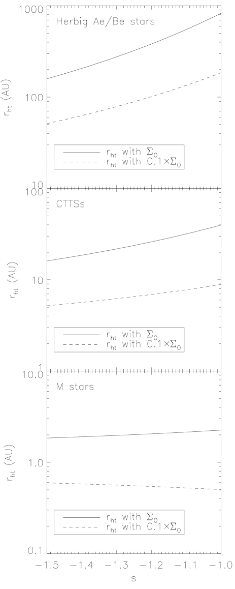
Figure 2: The heat transition radius as a function of the power-law index $s$. For all panels, the solid line denotes the case using the values in Table 3 while only $\Sigma_{0}$ decreases by a factor of 10 for the dashed line, which is the value used more often in the literature. In general, the radius increase with increasing $s$, since the quantity in the brackets of equation (3.26) is larger than unity. If it is less than unity (see the dashed line for the case of M stars), the radius decreases.

Table 4: The typical values of $r_{ht}$ for $\Sigma_{0}$

	Herbig Ae/Be stars	CTTSs	M stars
$r_{ht}$ (au) for $s=-3/2$	159	16	1.8
$r_{ht}$ (au) for $s=-1$	827	40	2.3

3.2.4 Ice lines: Origin of ice line barriers

We now discuss the effects of ice lines on temperature profiles which provide another barrier (Lyra et al., 2010). We note that our following approach is applicable to any other opacity transitions. We discuss them more in $\S$ 5.2. At the ice line, the number density of icy dust grains suddenly increases due to the low disc temperature. This sudden increment of dust provides an opacity transition. As a result, the temperature profile around the ice lines becomes shallow, resulting in inward migration while the profile well inside of the ice line becomes steep enough for planets to migrate outwards. Thus, planets migrating inwards are halted around the ice lines. This is known as the ice line barrier. This assumes that corotation torques are active -i.e. non-saturated, which is not necessarily clear at the ice lines (see $\S$ 4.4.1 and 5.2).

At first, we examine which heat source controls the location of ice lines, $r_{il}$. In order to proceed, we adopt equation (3.14) for viscous heating and equation (3.24) for stellar irradiation. Equating $T_{m}$ to the condensation temperature for H₂O ice, $T_{m,\mbox{H}_{2}\mbox{O}}(r_{il})=170$ K (Jang-Condell & Sasselov, 2004), equation (3.14) becomes

$$\frac{r_{il}}{r_{0}}=\left[T_{m,\mbox{H}_{2}\mbox{O}}^{10}(r_{il})\frac{64\sigma_{SB}\mu_{g}}{27\bar{\kappa}_{0}\Sigma_{0}^{2}\alpha\gamma k_{B}\Omega_{0}}\right]^{\frac{1}{2s-3/2}},$$ (3.27)

where $\bar{\kappa}=\bar{\kappa}_{0}T^{-7}$ with $\bar{\kappa}_{0}=2\times 10^{16}$ (Bell & Lin, 1994), and equation (3.24) becomes

$$\frac{r_{il}}{r_{0}}=\left(\frac{T_{m0}}{T_{m,\mbox{H}_{2}\mbox{O}}(r_{il})}\right)^{7/3}\left(\frac{R_{*}}{r_{0}}\right).$$ (3.28)

In general, the exponent index $s$ is negative, so that $r_{il}\propto\Sigma_{0}^{2/(3/2-2|s|)}$. This shows that as the surface density ($\Sigma_{0}$) decreases, the position of the ice line barriers moves inwards. We note that we examine the effects of a water-ice line here although the above argument is applicable to ice lines of any material by changing the relevant condensation temperature for species $k$, $T_{m,k}(r_{il})$. We will discuss them more in $\S$ 5.3.

Fig. 3 shows the above two equations as a function of $\alpha$ for discs around stars with various masses. We set $s=-1.5$, since this choice of $s$ minimises the importance of viscous heating in discs (see Fig. 2). The black, solid and dashed lines denote equation (3.27) with $\Sigma_{0}$ and $0.1\times\Sigma_{0}$, respectively while the dotted line is for equation (3.28). In all cases, $r_{il}$ defined by viscous heating is located at greater distances from the star than that by stellar irradiation. Furthermore, the transition radius defined by equation (3.26) is larger than any of these two radii (see the gray, thick lines). Thus, we can conclude that $r_{il}$ is determined by viscous heating for discs with a wide range of $\alpha$. This agrees with numerical work by Min et al. (2011) who showed the same results by numerically solving the full wavelength dependent, radiative transfer equation by means of a Monte Carlo method in 3D discs. In their simulations, viscous heating is explicitly included as well as stellar irradiation. In addition, this supports the findings of Lyra et al. (2010) who adopt disc models which are only heated by viscous heating. Furthermore, Fig. 3 shows that the radius of the heat transition is located outside of the ice line. This validates our choice of $\bar{\kappa}$ in equation (3.26).

We now investigate temperature profiles created by viscous heating around ice lines by adopting appropriate $\bar{\kappa}$ for each region (Bell & Lin, 1994). For the region inside of the ice lines, $\bar{\kappa}=\bar{\kappa}_{0}T^{1/2}$ with $\bar{\kappa}_{0}=0.1$. As a result, equation (3.14) becomes

$$T_{m}\propto r^{4s/5-3/5}$$ (3.29)

for discs with general $\dot{M}(r)$ (see equation (3.6)). $T_{m}\propto r^{-1.8}$ for the MMSN disc models ($s=-3/2$) while $T_{m}\propto r^{-1.4}$ for the disc models with $s=-1$. These steep profiles obviously indicate that planets migrate outwards. For the region around the ice lines, $\bar{\kappa}=\bar{\kappa}_{0}T^{-7}$ with $\bar{\kappa}_{0}=2\times 10^{16}$. Consequently, equation (3.14) becomes

$$T_{m}\propto r^{s/5-3/20}$$ (3.30)

for discs with $\dot{M}(r)$. $T_{m}\propto r^{-0.5}$ for the MMSN disc models ($s=-3/2$) while $T_{m}\propto r^{-0.4}$ for the disc models with $s=-1$. Under these shallow profiles, the entropy-related horseshoe drag cannot exceed the Linblad torque, and hence planets migrate inwards. Thus, a planet that migrates inwards beyond the ice line will be halted near the ice line due to this opacity transition.

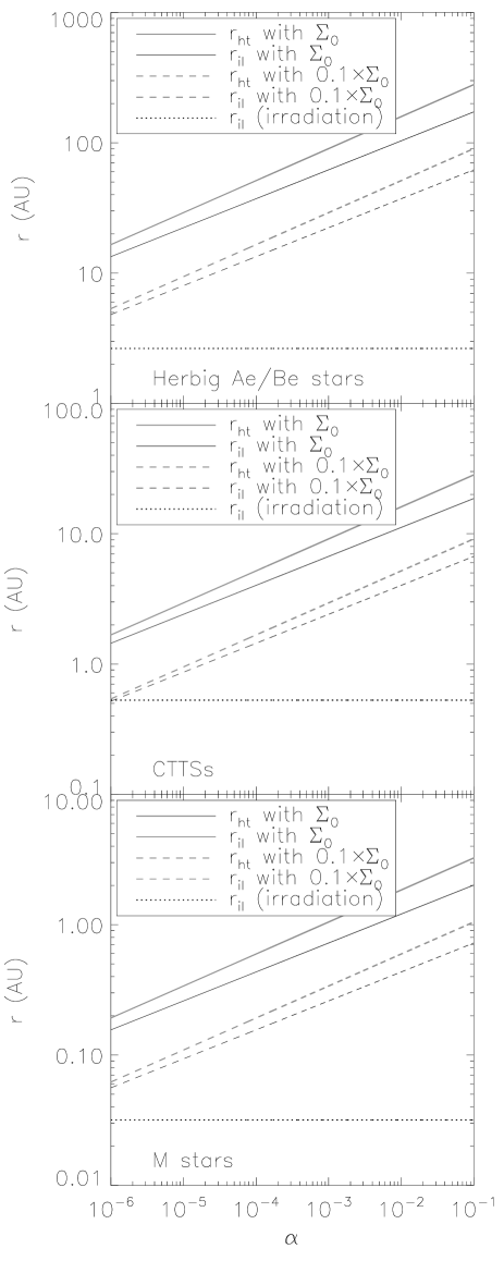
Figure 3: The location of the water-ice line as a function of the turbulence parameter, $\alpha$. For every panel, the solid and dashed, black lines denote the radius derived from viscous heating using $\Sigma_{0}$ and $0.1\times\Sigma_{0}$, respectively (see equation (3.27) and Table 3). The dotted lines are from stellar irradiation (see equation (3.28)). For comparison purposes, the heat transition radius is denoted by the two gray lines (see equation 3.26). For all panels, viscous heating defines the location of the water-ice lines. In addition, the heat transition radius is larger than that of the water-ice lines.

3.3 Comparison

We compare the heat transition barriers to the ice line barriers. We especially focus on the relative location of each barrier. As discussed above, Fig. 3 shows the relative location of these two barriers (see the black and gray lines). The ice line barrier (equation (3.27)) is located inside of the heat transition barrier (equation (3.26)) for discs with a wide range of $\alpha$. However, we again emphasise that the above analyses for these two barriers can be valid only for the disc region with ($10^{-1}\lesssim\alpha\lesssim 10^{-3}$). In the region with a low value of $\alpha$ such as dead zones ($\alpha\sim 10^{-5}$), any corotation torque will be saturated (i.e. zero), so that these two barriers are never activated there. We also note that for such low values of $\alpha$, ice lines can become barriers as a consequence of the Lindblad torque rather than the corotation torque. In addition, if the adiabatic approximation breaks down, which can arise for the late stage of disc evolution or the outer part of discs, these two mechanisms cannot be effective. We now examine the mechanisms of barriers activated by Lindblad torque.

4 Barriers arising from Linblad torques

Let us now examine regions wherein any torques arising from corotation resonances are negligible, so that the direction of migration is determined only by the Lindblad torque. Such regions occur for discs with a shallow temperature profile or a low value of $\alpha$ in dead zones ($\sim 10^{-5}$, HP10; Paardekooper et al., 2011; Masset & Casoli, 2010; Hasegawa & Pudritz, 2011).

4.1 Lindblad torque

4.1.1 Basic equations

We adopt analytical formulae of the Lindblad torques described in Hasegawa & Pudritz (2011, see their Appendix A for the complete expression). In the formulae, the standard Lindblad torque derived by Ward (1997) is modified, so that the vertical thickness of discs is taken into account without rigorously solving the 3D Euler equations. Thus, we treat the Lindblad torque density $d^{2}\Gamma^{L}/dzdr$ of a layer at the height $z$ from the mid-plane which is written as

$$\frac{d}{dz}\left(\frac{d\Gamma^{L}}{dr}(r,z)\right)=\epsilon\frac{2\mu^{2}\rho r_{p}^{4}\Omega_{p}^{4}}{r(1+4\xi^{2})\kappa^{2}}m^{4}\psi^{2},$$ (4.1)

where $\epsilon=+(-)$ for the outer(inner) resonances, the wavenumber $m$ is treated as a continuous variable;

$$m(r,z)=\sqrt{\frac{\kappa^{2}}{\left(\Omega-\Omega_{p}\right)^{2}-c_{s}^{2}/r^{2}}},$$ (4.2)

$\Omega_{p}=\sqrt{GM_{*}/r_{p}^{3}}$ is the angular velocity of a planet with $r=r_{p}$, the angular velocity $\Omega$ is

$$\Omega^{2}(r,z)=\Omega_{Kep}^{2}{\left(1+\frac{z^{2}}{r^{2}}\right)^{-3/2}}+\frac{1}{r\rho}\frac{\partial p}{\partial r},$$ (4.3)

the epicyclic frequency $\kappa$ is

$$\kappa^{2}(r,z)=\frac{1}{r^{3}}\frac{\partial}{\partial r}\left(r^{4}\Omega^{2}\right),$$ (4.4)

$\xi=mc_{s}/r\kappa$, and the forcing function $\psi$ is

$$\psi\approx\frac{\epsilon(\alpha_{r}^{2}-\zeta^{2}-1)}{2\alpha_{r}\sqrt{(\alpha_{r}-1)^{2}+\zeta^{2}}}K_{1}(\Lambda)+\left(\frac{\epsilon}{2m}+2\frac{\Omega}{\kappa}\sqrt{1+\xi^{2}}\right)\frac{K_{0}(\Lambda)}{\sqrt{\alpha_{r}}},$$ (4.5)

where

$$\Lambda(\alpha_{r},\zeta)=m\sqrt{\frac{(\alpha_{r}-1)^{2}+\zeta^{2}}{\alpha_{r}}},$$ (4.6)

$\alpha_{r}=r/r_{p}$ is the resonant position, and $\zeta=z/r$ (also see Table 1). We have adopted the standard approximation for $\psi$ (Goldreich & Tremaine, 1980; Jang-Condell & Sasselov, 2005). In addition, we have added a factor $\Omega/\kappa$ in the second term of $\psi$ following MG04.

Finally, the total torque exerted by the planets on discs is found by summing over all layers;

$$\Gamma^{L}=\int^{\infty}_{-\infty}dz\int^{\infty}_{0}dr\frac{d}{dz}\left(\frac{d\Gamma^{L}}{dr}(r,z)\right).$$ (4.7)

Note that the integration of equation (4.1) in terms of $z$ with $\zeta=0$ leads to the famous analytical formulae of the Lindblad torque density in 2D discs (Ward, 1997). Also, note that the tidal torques shown above are exerted by the planets on discs. Thus, the positive sign of $\epsilon$ in equation (4.1) means that the planets exert the tidal torques on discs, resulting in the loss of angular momentum from the planets and vice versa.

The validity of the above approach for mimicking the reduction of the tidal torques in 3D discs (Tanaka et al., 2002) is confirmed by Lubow & Ogilvie (1998) who showed that, in thermally stratified discs, 2D modes carry off more than 95 per cent of angular momentum and vertical modes are not dominant for transferring angular momentum between planets and their disc (also see Ward, 1988; Artymowicz, 1993; Jang-Condell & Sasselov, 2005).

4.1.2 Basic assumptions

We assume discs to be geometrically thin ($z=0$) and Keplerian. Under this assumption, we have

$$\rho \approx \frac{\Sigma}{H}$$ (4.8)

$$\Omega^{2} \approx \kappa^{2}\approx\Omega_{Kep}^{2},$$ (4.9)

$$\alpha^{3/2}_{r} \approx \left(1+\frac{\epsilon}{m}\sqrt{1+\xi^{2}}\right).$$ (4.10)

Thus, the torque density becomes

$$\frac{d}{dz}\left(\frac{d\Gamma^{L}}{dr}(r,z=0)\right)\approx\epsilon 2\mu^{2}GM_{*}\frac{m^{4}}{(1+4\xi^{2})}\frac{\Sigma\alpha_{r}^{2}\psi^{2}}{H},$$ (4.11)

where

$$\psi\approx\frac{1}{2}\left(1+\frac{1}{\alpha_{r}}\right)K_{1}(\Lambda)+\left(\frac{\epsilon}{2m}+2\sqrt{1+\xi^{2}}\right)\frac{K_{0}(\Lambda)}{\sqrt{\alpha_{r}}},$$ (4.12)

and

$$\Lambda=m\frac{|\alpha_{r}-1|}{\sqrt{\alpha_{r}}}.$$ (4.13)

Thus, the behavior of the torque density depends on $\Sigma\alpha_{r}^{2}\psi^{2}/H$. In the following subsections, we expand every quantity ($\alpha_{r},\Sigma,H,$ and $\psi$) as a series in $1/m(\ll 1)$, by assuming simple power-law disc structures in $\S$ 4.2 and non-power-law disc structures in $\S$ 4.3 and 4.4. This expansion is assured, since the torque takes the maximum value at $m\approx 10$ (Ward, 1997), and consequently, allows us to derive simple relations governing the direction of migration. Thus, we perform local analyses as done in $\S$ 2.

4.2 Simple power-law structures

We derive an analytical relation for the direction of planetary migration. Here, we assume simple power-law structures for the background density and temperature in discs, that is, $\Sigma\propto r^{s}$ and $T\propto r^{t}$. As a result, the relation depends only on the exponent of $\Sigma$ and $T$.

We can further simplify the mathematics by taking the limit $\xi\rightarrow 0$ (since the effect of gas pressure becomes negligible in the Keplerian discs; see Appendix B). Equation (4.11) then becomes, to first order in $1/m$,

$$\frac{d}{dz}\left(\frac{d\Gamma^{L}}{dr}(r,z=0)\right)\approx\epsilon\Gamma_{0}(r_{p})\left[1+\frac{2\epsilon}{3m}\left(s-\frac{t}{2}+\frac{1}{2}+\frac{5}{4}\right)\right],$$ (4.14)

where

$$\Gamma_{0}(r_{p})=2\mu^{2}GM_{*}\frac{\Sigma_{p}}{H_{p}}m^{4}\psi_{0}^{2}$$ (4.15)

Thus, the total torque is

$$\Gamma^{L} \approx \int^{\bar{H}_{p}}_{-\bar{H}_{p}}dz\Gamma_{0}(r_{p})\frac{4}{3m}\left(s-\frac{t}{2}+\frac{7}{4}\right)$$ (4.16)

$$= \frac{8}{3m}\Gamma_{0}(r_{p})\bar{H}_{p}\left(s-\frac{t}{2}+\frac{7}{4}\right),$$

where the integration range for $z$ is approximated to extend over the height of the photosphere $\bar{H}_{p}\sim 2H_{p}$ at the location of the planet since the density above the photosphere is about two orders of magnitude less than that at the mid-plane.

Consequently, the sign of the net torque depends on the sign expression;

$$\mbox{sgn}\left(s-\frac{t}{2}+\frac{7}{4}\right).$$ (4.17)

The torque becomes positive (inward migration) when $s-t/2+7/4>0$ and negative (outward migration) when $s-t/2+7/4<0$. When the MMSN disc models ($s=-3/2$) are adopted, $t>1/2$ is needed for outward migration while, when disc models have $s=-1$, $t>3/2$ is required. In general, $T$ is a decreasing function of $r$. Therefore, some specific features in discs are required for the Lindblad torque to excite barriers. In the following subsections, we focus on dead zones and ice lines.

4.3 Dead zone barriers

Dead zones are known to play very interesting roles in planetary formation and migration (e.g. Matsumura & Pudritz, 2006). They can excite two barriers: density barriers (MPT07) and thermal barriers (HP10). These two barriers are interesting products of turbulent transitions. In this subsection, we derive the analytical relation which predicts when the direction of migration is reversed from inwards to outwards for these cases.

4.3.1 Thermal barriers

Thermal barriers were uncovered by HP10 who first investigated numerically the effects of dead zones on the temperature structure of discs (also see Hasegawa & Pudritz, 2010b). In their paper, the temperature structure of discs with dust settling and a dead zone was simulated by solving the full wavelength dependent, radiative transfer equation by means of a Monte Carlo method. Stellar irradiation is assumed to be the main heat source. HP10 demonstrated that planets migrate outward in a region where a positive temperature gradient is established (see their figs 1 and 3). This temperature gradient is a result of the back heating of the dead zone by a thermally hot dusty wall, and is well represented by $T\propto r^{t^{\prime}}$ with $t^{\prime}\gtrsim 3/2$. The hot dusty wall is produced by the enhanced dust settling in the dead zone and the resultant enhanced absorption of stellar irradiation by the wall. Since they adopted $\Sigma\propto r^{s}$ with $s=-1$, the profile of the positive temperature gradient is identical to the profile required by equation (4.17) in order for planets to migrate outwards. Thus, our relation predicts the results of the detail numerical simulations very well.

4.3.2 Density jumps

Density barriers were found by MPT07 who undertook a pioneering study on the effects of dead zones on planetary migration. They are created by the formation of a density jump at the outer edge of dead zones which arises as a consequence of time-dependent, viscous evolution of discs (also see Matsumura et al., 2009, for a more complete study). This density jump develops because of the huge difference in the strength of turbulence ($\alpha$) between the active and dead zones of the disc.

Here, we analytically derive an analogous relation for density barriers. We adopt equation (3.1) as the background surface density. In this case, $F_{g}$ is the density difference between the active and dead zones, $r_{trans}=r_{edge}$ is a orbital radius of the outer boundary of the dead zone, and $\omega=cH$ is the width of the transition (also see Table 1). Except for this, we adopt the same approximation as above. As a result, the relation depends on the structure of the dead zones as well as the exponent of $\Sigma$ and $T$. Since planets are slowed down or stopped near $r_{edge}$, we can approximate $r_{edge}\approx r_{p}$.

We note that a slightly more accurate shape of the boundary in equation (3.1) can be expressed in terms of error functions. However, the difference between the error and $\tanh$ functions is less than 1 per cent with the proper choice of coefficients (Basset, 1998). Furthermore, $\tanh$ functions are fully analytical. For these reasons, we adopt $\tanh$ functions.

Adopting the same approximation as above, we find

$$\Sigma/\Sigma_{int}\approx 1+\frac{F_{g}-1}{2}\left[1-\tanh\left(\frac{\epsilon}{c}\right)+h_{p}\frac{t+3}{2c}\frac{1}{\cosh^{2}(\epsilon/c)}\right].$$ (4.18)

Note that we expanded $\Sigma$ in terms of $1/m$ and finally expressed it in terms of $h_{p}$ assuming

$$h_{p}\approx\frac{2}{3m}.$$ (4.19)

This is reasonable because the resonant positions are pushed away from the planet by a distance $\sim H(=rh)$ due to the gas pressure (Artymowicz, 1993; Ward, 1997, also see equation (4.10)).

Inserting the above surface density into equation (4.11), the sign of the net torque consequently becomes

$$\mbox{sgn}\left[-(F_{g}-1)\tanh\left(\frac{1}{c}\right)+(F_{g}+1)h_{p}\left(s-\frac{t}{2}+\frac{7}{4}\right)\right].$$ (4.20)

Again, we can check the validity of equation (4.20) by comparing it with the numerical simulations. In this case, we compare the results of MPT07. Changing parameters $F_{g}$ and $c$ in equation (3.1), they investigated what values of $F_{g}$ and $\omega$ result in outward migration (see their Appendix B). Table 5 summarises their experiments with our predictions (given in the brackets). One observes immediately that equation (4.20) well explains the results of their numerical simulations. One might wonder if the corotation torque is significant around the density jump, but this is not the case. MPT07 clarified that planets migrate outwards due to the reversal of the balance of Lindblad torques, not corotation torques. This arises because the Lindblad resonant positions are located further away from planets than the corotation ones. Therefore, migrating planets first encounter the inner Lindblad torque at the density jump and this is sufficient to reverse the direction of migration.

In summary, both our simple analytical relations (equations (4.17) and (4.20)) well reproduce the results of the detailed numerical simulations of dead zones as planet traps. This indicates that our assumptions and treatments are reasonable to capture the physics arising in the more complicated numerical simulations.

Table 5: Summary of parameter study

	$F_{g}$=5	$F_{g}$=10	$F_{g}$=100
$c=4$	in (0.07)	in (-0.28)	out (-6.6)
$c=2$	out (-0.8)	out (-2.2)	out (-28)
$c=1$	out (-2)	out (-4.9)	out (-57)

$h_{p}$=0.35, $s$=-3/2, and $t$=-1/2. in(out) means the inward(outward) migration calculated by MPT07. The number in the brackets is calculated from equation (4.20).

4.4 Ice line barriers

We finally examine ice line barriers. As discussed in $\S$ 3.2.4, the disc radius of the ice lines is determined by viscous heating for a wide range of $\alpha$ (see Fig. 3). In this subsection, we discuss how ice lines establish layered structures, and derive analytical relations for the resultant barrier. Thus, we investigate ice lines as an example of opacity and turbulent transitions. Again, we specify a ice line due to water, although all our analyses are applicable to ice lines of any material. The discussion is presented in $\S$ 5.3.

4.4.1 Layered structures at ice lines

As mentioned before, the number density of icy grains suddenly increases at the ice lines. If discs are considered to be turbulent due to the MRI, this sudden increment of dust can result in layered structures: the MRI active, surface layer and the MRI dead, inner layer (Gammie, 1996). This can be understood as follows. At the ice lines, the number density of free electrons in the disc also suddenly drops because they are absorbed by such dust grains. Since free electrons are the main contributor of coupling with magnetic fields threading the disc (Sano et al., 2000), the surface density of the MRI active region is strongly diminished, and consequently the surface density of the MRI dead region is enhanced. As a result, a density bump appears which acts as a barrier (see Fig. 4). Thus, the mean value of $\alpha$ around the ice lines becomes $\alpha\simeq\alpha_{D}$ (see equation (4.21)), and hence, the ice lines can be regarded as a self-regulated, localised dead zone. In summary, the subsequent process initiated by icy grains can reduce the value of $\alpha$ at the ice lines. The disc radius at which it appears is determined by viscous heating (see equation (3.27)).

We recall from $\S$ 3.2.4 that ice lines become a barrier due to the corotation torque (also see IL08). However, any corotation torque may saturate at the ice lines because the turbulence dies out there - a conclusion which is valid for any disc in which turbulence is excited by the MRI. If the MRI is the most general source of disc turbulence, we expect that the ice lines may be natural barriers arising from the Lindblad torques rather than corotation torques.

4.4.2 Disc models

We adopt a parameterised treatment of dead zones in a disc described by IL08. In the region with layered structures, the effective $\alpha$ can be generally written as

$$\alpha=\frac{\Sigma_{A}\alpha_{A}+(\Sigma-\Sigma_{A})\alpha_{D}}{\Sigma},$$ (4.21)

where $\Sigma_{A}$ is the surface density of the active layer, and $\alpha_{A}$ and $\alpha_{D}$ are the strength of turbulence in the active and dead layers, respectively (Kretke & Lin, 2007; Matsumura et al., 2009, also see Table 1). Assuming stationary accretion discs (see equation (3.6)) with equation (4.21), the surface density is given as

$$\Sigma=\frac{\dot{M}}{3\pi c_{s}H\alpha_{D}}-\Sigma_{A}\frac{\alpha_{A}-\alpha_{D}}{\alpha_{D}},$$ (4.22)

where $\Sigma_{A}$ cannot exceed $\Sigma$. Thus, equation (4.22) is useful for representing the surface density within dead zones where $\Sigma_{A}<\Sigma$. Also, this equation implies that the structure of $\Sigma$ in the dead zones strongly depends on $\Sigma_{A}$. However, the structure of $\Sigma_{A}$ is not well constrained by theory, since it is very sensitive to the distribution of dust grains as well as the chemical models (Sano et al., 2000; Ilgner & Nelson, 2006). Therefore, we adopt simple prescriptions proposed by Kretke & Lin (2007) and IL08 as follows. For the active region where $\Sigma_{A}\approx\Sigma$, the surface density simply becomes

$$\Sigma=\frac{\dot{M}}{3\pi c_{s}H\alpha_{A}},$$ (4.23)

if there is no ice line. The effects of the ice lines on $\Sigma$ are described below.

4.4.3 Density jumps without ice lines

At first, we examine density barriers produced by dead zones (see equation (4.22)) to compare the our previous analysis done in $\S$ 4.3. For the surface density of the active layer, we assume

$$\Sigma_{A}=\Sigma_{A0}f_{ice}\left(\frac{r}{r_{0}}\right)^{s_{A}}$$ (4.24)

following Kretke & Lin (2007). We note that $\Sigma_{A0}$ and $f_{ice}$ are very sensitive to the dust distribution (also see Table 1). However, we set $\Sigma_{A0}$ constant and $f_{ice}=1$ here. A more detailed analysis is presented below where the effects of ice lines on $f_{ice}$ are included. In discs with layered structures, it is generally considered that $s_{A}\geq 0$.

Using the above equation, equation (4.22) is approximately written as

$$\Sigma \simeq \frac{\dot{M}}{3\pi\alpha_{D}H_{p}^{2}\Omega_{p}}\left(1-\epsilon h_{p}\left(t+\frac{3}{2}\right)\right)$$

$$-\Sigma_{A}(r_{p})\frac{\alpha_{A}-\alpha_{D}}{\alpha_{D}}\left(1+\epsilon s_{A}h_{p}\right),$$

where we performed Taylor expansion of $\Sigma$ in terms of $1/m$, and finally expressed it by $h_{p}$, assuming $h_{p}\approx 2/3m$. Thus, the direction of migration is determined by

$$\mbox{sgn}\left[\frac{\dot{M}}{3\pi\alpha_{D}H_{p}^{2}\Omega_{p}}h_{p}\left(-\frac{3}{2}t+\frac{1}{4}\right)\right.$$ (4.26)

$$\left.-\Sigma_{A}(r_{p})\frac{\alpha_{A}-\alpha_{D}}{\alpha_{D}}h_{p}\left(s_{A}-\frac{t}{2}+\frac{7}{4}\right)\right].$$

Since the outer edge of dead zones where a density jump develops is established around the region with $\Sigma_{A}\sim\Sigma/2$ , we can assume

$$\Sigma_{A}(r_{p})\frac{\alpha_{A}-\alpha_{D}}{\alpha_{D}}\approx\frac{\dot{M}}{3\pi\alpha_{D}H_{p}^{2}\Omega_{p}}\frac{\alpha_{A}-\alpha_{D}}{\alpha_{A}+\alpha_{D}}.$$ (4.27)

We emphasise that equation (4.27) gives the position of planets halted by the density barrier which defines the outer edge of the dead zones ($r_{p}\approx r_{edge}$). In addition, this equation is another expression that the necessary condition ($\Sigma_{A}<\Sigma$) is safely satisfied. As a result, the sign of the net torque is written as

$$\mbox{sgn}\left[s_{A}-\frac{t}{2}+\frac{7}{4}-\frac{\alpha_{A}+\alpha_{D}}{2\alpha_{D}}\left(s_{A}+t+\frac{3}{2}\right)\right].$$ (4.28)

Compared with equation (4.17), the layered structure with a density jump gives an additional term which controls the direction of migration (since $\alpha_{A}\gg\alpha_{D}$). Thus, planets migrate inwards when sgn$(s_{A}+t+3/2)<0$ while they migrate outwards when $s_{A}+t+3/2>0$. In standard disc models, $s_{A}>0$ and $t\simeq-1/2$. Our relation therefore dictates outward migration, which is also consistent with our previous analysis done in $\S$ 4.3.2.

4.4.4 Density jumps with ice lines

We incorporate the effects of ice lines on the surface density of the active layer, following IL08 (see Fig. 4). In this case, we need to consider two separate cases, depending on the ratio of $r_{il}$ to $r_{edge}$, where $r_{il}$ is the disc radius of an ice line. For the case that $r_{il}/r_{edge}<1$, we can use equations (4.22) and (4.24) as the surface density while we need to modify equation (4.23) for the case that $r_{il}/r_{edge}>1$.

We first examine the case that $r_{il}<r_{edge}$, that is, an ice line is located inside of a dead zone. In this case, $f_{ice}$ in equation (4.24) is generally given as

$$f_{ice}=f_{d}\left[1+\frac{f_{d1}}{2}\left(1+\tanh\left(\frac{r-r_{il}}{w}\right)\right)\right]^{-1},$$ (4.29)

where $f_{d}$ and $f_{d1}$ parameterise the effects of an ice line at which the surface density of the active layer suddenly drops. As noted by Kretke & Lin (2007), the surface density distortion induced by ice lines produces a radial, positive pressure gradient there, and consequently dust can be trapped there. Otherwise, it migrates inwards due to the so-called head winds arising from the gas motion (Weidenschilling, 1977). Since the maximum migration speed of dust is $\sim 1/\alpha$ times faster than the viscous evolution of gas, dust is quickly piled up at the ice lines. This effect can be included in $f_{d}$ which is generally written as

$$f_{d}=\left[1+f_{d2}\exp\left(-\left(\frac{r-r_{il}}{w}\right)^{2}\right)\right]^{-1}.$$ (4.30)

We note that inclusion of the dust effects may upgrade the ice line barriers to planet traps although we keep calling them barriers.

Fig. 4 shows the typical $\Sigma$ (as controlled by equations (4.29) and (4.30)) and the role of the parameters $f_{d1}$ and $f_{f2}$ in $f_{ice}$ .

Consequently, we can approximate the surface density (see equations (4.22), (4.24), (4.29), and (4.30)) as

$$\Sigma \simeq \frac{\dot{M}}{3\pi H_{p}^{2}\Omega_{p}\alpha_{D}}\left(1-\epsilon h_{p}\left(t+\frac{3}{2}\right)\right)$$

$$-\Sigma_{A}(r_{p},f_{ice}=1)\frac{\alpha_{A}-\alpha_{D}}{\alpha_{D}}D,$$

where

$$D = AB+\epsilon h_{p}$$

$$\times \left(B\left(As_{A}+\epsilon\frac{t+3}{2c}\frac{f_{d1}}{2}\frac{1}{\cosh^{2}(1/c)}\right)-A(B-1)\frac{t+3}{c^{2}}\right),$$

$$A=1+\frac{f_{d1}}{2}\left(1+\epsilon\tanh\left(\frac{1}{c}\right)\right)\equiv A_{1}+\epsilon A_{2},$$ (4.33)

and

$$B=1+f_{d2}\exp\left(-\frac{1}{c^{2}}\right).$$ (4.34)

We emphasise that the location of the ice line barrier which can halt planets migrating inward ($r_{p}\approx r_{il}$) is determined by viscous heating (see equation (3.27)) while the location of the density barrier produced by dead zones ($r_{p}\approx r_{edge}$) is determined by equation (4.27).

As a result, the sign of the net torque is given as

$$\mbox{sgn}\left[\frac{\dot{M}}{3\pi H_{p}^{2}\Omega_{p}\alpha_{D}}h_{p}\left(-\frac{3}{2}t+\frac{1}{4}\right)-\Sigma_{A}(r_{p},f_{ice}=1)\frac{\alpha_{A}-\alpha_{D}}{\alpha_{D}}E\right],$$ (4.35)

where

$$E = A_{2}\left(B-(B-1)\frac{t+3}{c^{2}}\right)$$

$$+ h_{p}A_{1}\left[B\left(s_{A}-\frac{t}{2}+\frac{7}{4}\right)-(B-1)\frac{t+3}{c^{2}}\left(-\frac{t}{2}+\frac{7}{4}\right)\right].$$

The above equation is identical to equation (4.4.3) if $A_{1}$ and $B$ $\rightarrow 1$, and $A_{2}\rightarrow 0$ (equivalently, $f_{d1}$ and $f_{d2}$ $\rightarrow 0$). Before fully examining equation (4.35) which looks very complicated, it is very useful to understand a simplified case. Taking the leading terms, outward migration arises when

$$\Sigma_{A}(r_{p},f_{ice}=1)>\frac{\dot{M}}{3\pi(\alpha_{A}-\alpha_{D})}\frac{1}{r_{p}c_{s}(r_{p})}.$$ (4.37)

The relation shows that the ice line barrier is readily active for discs with low accretion rate, high disc temperatures, high surface density of the active region, and large disc radii of the ice lines ($r_{p}\approx r_{il}$). In addition, this relation is very useful for constraining the effectiveness of the ice line barrier, which is discussed more in the next subsection.

We can readily solve the equation (4.35), since it is quadratic in $t$. Fig. 5 shows $r_{il}$ as a function of $t$. The black lines denote the negative solution while the gray, thick lines are for the positive solution. The regions where planets migrate outwards are encompassed by one of the solutions, $x-$ and, $y-$axes (labeled by Outward). In this figure, we set $f_{d1}=6$, $f_{d2}=2$, $s_{A}=3$, and $\Sigma_{A0}/\Sigma_{0}=0.01$ at $r_{0}=1$ au following IL08 (also see Table 3). We consider a water-ice line, so that $T_{m,\mbox{H}_{2}\mbox{O}}(r_{il})=170$ K (Jang-Condell & Sasselov, 2004). We use $c=1$, because any sharp transition in discs is smoothed out by disc viscosity (Yang & Menou, 2010). For stellar parameters, we adopt the values of CTTSs (see Table 3). This disc setup is our fiducial model (see the solid lines). Based on equation (4.37), the choice of stellar parameters ($R_{*}$ and $T_{*}$) does not matter if $r_{il}$ is parameterised (see equations (3.24) and (3.27)). Although the complete treatment in which $r_{il}$ depends on stellar parameters is presented in $\S$ 6, we simply label $r_{il}$ by asterisks for comparison purposes here (see equation (6.1)).

In Fig. 5, we explore parameter space by changing $\dot{M}$, $\Sigma_{A0}$, and $s_{A}$ (on the top, middle, and bottom panels). For $t<$0 which is general for any disc, higher $\dot{M}$ and $s_{A}$, and lower $\Sigma_{A0}$ reduce the outward migration region. This is consistent with the above argument (see equation (4.37)). The situation is the opposite for $t>$0 which can happen due to hot dusty walls. If the dependence of $r_{il}$ on $\dot{M}$ is taken into account (see the top panel), higher accretion rates do not necessarily reduce the region where the water-ice line barrier is active. This arises because higher accretion rates result in larger water-ice line radii which are preferred for outward migration (see equation (4.37)). Thus, the conditions for outward migration are controlled by the complex dependence on $\dot{M}$. Another interesting feature is shown in the bottom panel. Around $r_{il}\approx$ 30 au with $t>0$, both negative and positive solutions merge with each other (see the black and gray dotted lines on the bottom panel). This happens because there is no solution to equation (4.35).

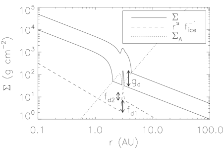
Figure 4: The typical structures of $\Sigma$ and $\Sigma_{A}$ controlled by $f_{ice}$. The upper solid line denotes the case that an ice line is located within a dead zone while the lower solid line is for an ice line beyond the dead zone. The distribution of $\Sigma_{A}$ is denoted by the dotted line. The definitions of $f_{d1}$ and $f_{d2}$ in $f_{ice}$ and of $g_{d}$ in $\Sigma$ are labeled in the figure.

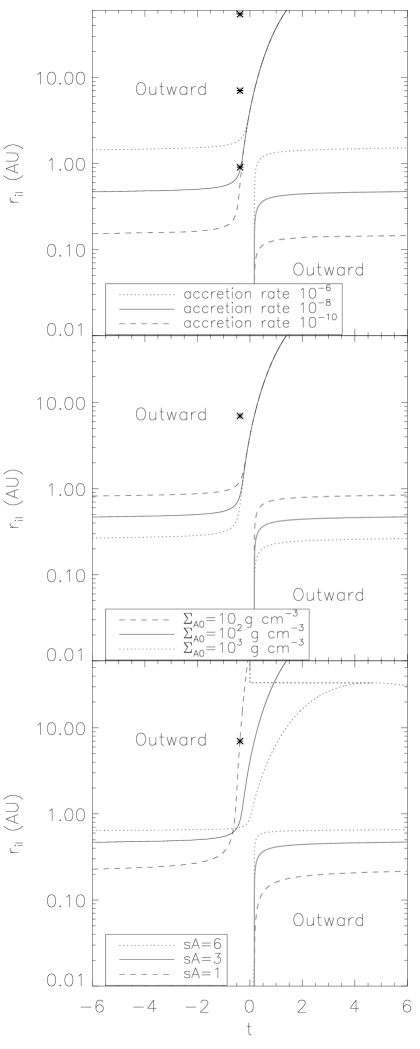
Figure 5: The location of a water-ice line as a function of the temperature exponent $t$. The black lines denote the negative solution to equation (4.35) while the gray, thick lines are for the positive solution. The regions where planets migrate outwards are surrounded by one of the solutions and $x-$ and $y-$axes (labeled by Outward). For the top, middle, and bottom panels, $\dot{M}$, $\Sigma_{A0}$, and $s_{A}$ are varied, respectively. Otherwise, we adopt the values of the fiducial model. For the case of $t<0$ with higher $\dot{M}$ and $s_{A}$ and lower $\Sigma_{A0}$, the outward migration region shrinks. For the case of $t>0$ the situation is the opposite. For comparison purposes, we label $r_{il}$ by asterisks (see equation (6.1)). For the top panel, the value of $r_{il}$ increases with increasing $\dot{M}$. This indicates that the conditions for outward migration are determined by the complex dependence on $\dot{M}$ (see equation (4.37)).

Now, we examine the case that $r_{il}/r_{edge}>1$, that is, an ice line is located beyond the dead zone in the active region of the disc. In this case, we adopt the following functional form for $\Sigma$;

$$\Sigma=\frac{\dot{M}}{3\pi c_{s}H\alpha_{A}}\left[1+g_{d}\exp\left(-\left(\frac{r-r_{il}}{w}\right)^{2}\right)\right].$$ (4.38)

Compared with equation (4.23), the ice line produces a density bump at $r=r_{il}$ which is a consequence of a localised layered structure. This function well represents the results of IL08 with a proper choice of $g_{d}$ (see the lower solid line in Fig. 4). Here, we only examine the power-law index of $\Sigma$ rather than expanding it in terms of $h$. This is because one of our approximations, $r_{p}\approx r_{il}$, limits the applicability to Gaussian-functions. In fact, planets migrating towards the density bump can be halted around $r_{p}=r_{il}+\vartriangle r$ where a negative steep surface density profile plays the critical role. However, the assumption that $r_{p}\approx r_{il}$ washes out this effect. This also indicates that equation (4.35) may underestimate the required condition.

The power-law index of $\Sigma$ is given as

$$\bar{s}\equiv\frac{d\ln\Sigma}{d\ln r}=-t-\frac{3}{2}-\frac{\frac{2r_{p}(r_{p}-r_{il})}{w^{2}}g_{d}\exp\left(-\left(\frac{r_{p}-r_{il}}{w}\right)^{2}\right)}{1+g_{d}\exp\left(-\left(\frac{r_{p}-r_{il}}{w}\right)^{2}\right)}.$$ (4.39)

We recall that $\bar{s}$ becomes equivalent to $s$ for pure power-law discs (see equation (3.2)). Assuming planets to be halted around $r_{p}\approx r_{il}+w\sqrt{\ln 2}$ where the Gaussian function takes half of the maximum value, the resultant value of $\bar{s}$ becomes

$$\bar{s}=-t-\frac{3}{2}-\frac{\frac{g_{d}}{ch_{p}}\sqrt{\ln 2}}{1+g_{d}/2}.$$ (4.40)

As a result, we find that the direction of migration is controlled by

$$\mbox{sgn}\left(\bar{s}-\frac{t}{2}+\frac{7}{4}\right),$$ (4.41)

where we have assumed any disc quantity to behave as power-law in a local region centered at $r\approx r_{p}$ (see $\S$ 4.2). For discs with $h_{p}=0.1$, $c=1$, and $g_{d}=3$, $t>-6.5$ is required for outward migration while for discs with $h_{p}=0.1$, $c=1$, and $g_{d}=6$, $t>-8.2$ is needed. Thus, the direction of migration is readily reversed by the density bump produced by the ice lines. Furthermore, larger density bump $g_{d}$ expands the outward migration region, as expected.

4.5 Locations of the barriers

We can now compare the dead zone and ice line barriers in order to examine the relative importance of each. We adopt the analysis done for the case of $r_{il}/r_{edge}$. We especially focus on the relative location of each barrier. Combining two equations (4.27) and (4.37), we find the condition which is given as

$$\frac{r_{il}}{r_{edge}}>\left(h(r_{edge})\frac{\alpha_{A}+\alpha_{D}}{\alpha_{A}-\alpha_{D}}\right)^{\frac{1}{s_{A}+t/2+1}},$$ (4.42)

where we set $r_{0}=r_{edge}$. If this condition is satisfied, the ice line and density barriers are both active while if not, only the density barrier is active. Thus, the separation between the ice line and dead zone barriers is required to be relatively small in order for the ice line barrier to be effective. Table 6 summarises the threshold values of $r_{il}/r_{edge}$ for various $s_{A}$, $t$, and $h(r_{edge})$. As all three quantities increase, the threshold values of $r_{il}/r_{edge}$ increase. In other words, the parameter space where the ice line barrier is effective is larger for lower values of $s_{A}$, $t$, and $h(r_{edge})$. More complete treatments in which the ice line radius is determined by viscous heating are presented in $\S$ 6.

Table 6: The condition for the ice line barrier to be active

($s_{A}$,$t$,$h(r_{edge})$)	(3,-1/2,0.01)	(3,-1/2,0.1)	(3,-1/2,1)
$r_{il}/r_{edge}$	0.2	0.5	1
($s_{A}$,$t$,$h(r_{edge})$)	(3,-1.5,0.1)	(3,-1/2,0.1)	(3,1.5,0.1)
$r_{il}/r_{edge}$	0.4	0.5	0.7
($s_{A}$,$t$,$h(r_{edge})$)	(1,-1/2,0.1)	(3,-1/2,0.1)	(6,1/2,0.1)
$r_{il}/r_{edge}$	0.2	0.5	0.7

5 Discussion

Before we integrate our analyses into a coherent picture, we discuss other possible barriers induced by other physical processes which are neglected in this paper. Also, we discuss opacity transitions that are neglected in our unified picture. In addition, we examine the possibility of molecules other than water to excite ice line barriers. Finally, we estimate the mass range in which planets are regarded as type I migrator.

5.1 Other possible barriers

We have so far assumed that stellar irradiation heats up only the dust in discs. However, photons emitted from stars, especially with very short wavelengths such as UV and X-rays can heat up the gas. This results in the photoevaporation of discs (Hollenbach et al., 1994; Johnstone et al., 1998) - which considerably affects planet formation and migration (e.g. Mordasini et al., 2009). Lyra et al. (2010) showed that photoevaporation can activate another barrier. This arises by the reduction of the surface density of gas due to photoevaporation. Since viscous heating strongly depends on the surface density (see equation (3.14)), this reduction results in shallower temperature profiles. Consequently, planets are halted at the region where the transition of the temperature slope occurs.

In general, photoevaporation is considered to be important for discs surrounded by nearby OB associations which provide a huge input of high energy photons. In addition to photoevaporation, one expects that such massive stars can significantly affect the disc structure by changing the dust temperature. Recently, Gorti & Hollenbach (2009) have shown that, without nearby massive stars, even low-mass central stars ($>0.3M_{\oplus}$) can drive photoevaporation of their surrounding discs ($r\gtrsim 20$ au). This arises from energetic stellar irradiation (far-UV, extreme-UV, and X-rays). We will address this in a future publication.

In addition, we neglect the effects of the inner edge of dead zones where a positive radial gradient of the surface density can form. Such a profile can produce a barrier due to the vortensity-related corotation torque. However, the disc radius of the inner edge of dead zones can be fixed around $r\approx 0.01$ au, because the radius is controlled by the thermal ionisation temperature of gas. Thus, the barrier is unlikely to play an important role in the diversity of the detected exoplanetary systems. For the reason, we disregard it in this paper.

5.2 Neglect of opacity transitions

We have intensively investigated ice lines as an opacity transitions in $\S$ 3.2.4 while our approach is applicable to any other opacity transitions. In general, protoplanetary discs have several opacity transitions. MG04 showed that any opacity transition (including ice lines) affects the disc surface density and temperature in a similar fashion. Therefore, it is naturally expected that a single disc can have several barriers that are all excited by opacity transitions. Nonetheless, we will neglect all opacity transitions in $\S\ref{synthesis}$ for the following reasons.

Except for those produced by ice lines, all opacity transitions are a consequence of the high disc temperatures and subsequent destruction of opacity sources. As a result, their disc radii distribute well inside of 1 au (see fig. 1 of MG04). MG04 found that these opacity transitions make the migration time significantly longer due to the Lindblad torque alone. (Equivalently, the net torque exerted on a planet becomes a very small (in magnitude), negative value.) This indicates that, in order to actually stop the planet’s inward migration, a small amount of outward-directed corotation torque would be needed. However, any corotation torque at the opacity transitions is likely to vanish due to the presence of dead zones. As discussed above, protoplanetary discs may have dead zones that are 1- 10 au in size from their central stars, depending on their column density. One of the key features of the dead zones is a low level of turbulence, which results in the saturation (ineffectiveness) of corotation torques there (see $\S$ 4). Thus, opacity transitions within dead zones cannot be planet traps and therefore we disregard opacity transitions other than those created by ice lines. For the ice lines, it is more likely that the process initiated by the increment of icy dust grains reduces a level of turbulence there and hence ice lines are regarded as localised dead zones (see 4.4.1). Thus, we include ice lines as an opacity and turbulent transition rather than an opacity transition in $\S$ 6. In summary, any opacity transition is neglected below.

5.3 Ice lines of other molecules

We have focused on a water-ice line in the above discussions, although our analyses apply to ice lines of any molecules in discs. It is well known that water is not the most abundant chemical species in protoplanetary discs (e.g. Aikawa & Herbst, 1999). In general, CO is the most abundant molecule in discs. Davis (2007) showed that the total amount of CO-ice is much larger than water-ice in irradiated accretion discs. Furthermore, different species have different condensation temperatures. Davis (2005) demonstrated that the location of ice lines strongly depends on molecules in consideration. Thus, it is very interesting to investigate which molecules can produce barriers in discs.

In order to proceed, we adopt the analyses done in $\S$ 4.4. We especially focus on the minimum abundance of molecules which is required for their ice lines to be a barrier. We present the detail analysis in Appendix C and summarise our findings here. We find that whether or not ice lines of other molecules act as barriers strongly depends on the disc parameters such as $s_{A}$ and $t$. Adopting reasonable values for them, we find that, for molecules that condense within a dead zone, only specific, abundant species such as CO have the possibility to work as a barrier. If molecules freeze out beyond the dead zone, then even a tiny fraction of the molecules can act as a barrier. In summary, other molecular species can produce ice lines but these will form near to the position of the outer edge of the dead zone ($r_{edge}$). We leave more comprehensive models for ice lines to a future publication. In the following discussions, we again assume water-ice to be abundant enough for creating a barrier.

5.4 Mass limits for type I migration

We discuss the mass limits that our analyses apply to. Type I migration is only applicable to low mass protoplanets. Massive protoplanets can open up a gap in their discs and undergo type II migration. This mode of migration is controlled by viscous evolution of discs and is much slower than the type I migration. The critical mass, also known as the gap-opening mass, is well discussed in the literature (e.g. Matsumura & Pudritz, 2006), and given by

$$\frac{M_{p,max}}{M_{*}}=\mbox{min}\left[3Ch_{p}^{3},C\sqrt{40\alpha h_{p}^{5}}\right],$$ (5.1)

where we have introduced a coefficient $C=3$ into the original condition by taking into account the reduction of the tidal torque due to the disc thickness (Hasegawa & Pudritz, 2011). The left term in the brackets of equation (5.1) is derived by a Hill radius analysis while the right term for viscous ones. Table 7 summarises $M_{p,max}$ for stars with various masses at $r_{p}=1$ au. The stellar and disc parameters are given in Table 3. For discs with $\alpha=10^{-2}$, the critical mass is established by the Hill radius analysis, and has the same order of Neptune to Saturn masses. On the other hand, the criterion derived for viscous discs provides the gap-opening mass for discs with $\alpha=10^{-5}$, and $M_{p,max}$ is on the order of Earth masses.

What is the minimum mass for protoplanets to undergo type I migration? It is interesting that the dynamics of low mass bodies, from dust grains to planetesimals, can drastically differ from that of protoplanets (Adachi et al., 1976; Bai & Stone, 2010; Nelson & Gressel, 2010). This arises mainly from gas drag. One of the most famous consequences of the gas drag is the rapid inward migration of meter-sized particles discussed in $\S$ 4.4.4. The size dependency of gas drag affects the formation of planetesimals (see Chiang & Youdin, 2010, for a recent review). However, we simply focus on the dynamics of planetesimals, since we are interested in minimum mass of type I migrator. In laminar discs, the rate of change of semi-major axis induced by gas drag is given by (see Adachi et al., 1976, for derivation)

$$\frac{dr_{p}}{dt}\simeq-K_{drag}\frac{\rho_{p}r_{p}^{2}\Omega_{p}}{M_{p}^{1/3}},$$ (5.2)

where $K_{drag}$ is a function of the eccentricity, the inclination, and the material density of a planetesimal, and the radial pressure gradient of discs. Following Kokubo & Ida (2000), we find $K_{drag}\sim 2.7\times 10^{-5}$ in cgs units. As a result, the timescale of gas drag is written as

$$\tau_{drag}\simeq r_{p}\left|\frac{dr_{p}}{dt}\right|^{-1}=\frac{M_{p}^{1/3}h_{p}}{K_{drag}\Sigma_{p}\Omega_{p}},$$ (5.3)

where we have assumed $\rho_{p}\simeq\Sigma_{p}/H_{p}$. On the other hand, the migration timescale is generally written as

$$\tau_{mig}\simeq\frac{M_{p}r_{p}^{2}\Omega_{p}}{2\Gamma},$$ (5.4)

where the tidal torque is scaled by

$$\Gamma=K_{mig}\left(\frac{M_{p}}{M_{*}}\right)^{2}\frac{\Sigma_{p}r_{p}^{4}\Omega_{p}^{2}}{h_{p}^{2}},$$ (5.5)

and $K_{mig}$ is an order of 1 to 10, depending on disc models (Paardekooper et al., 2010). Equating equation (5.3) with equation (5.4), the critical mass is given as

$$M_{p,min}=\left(\frac{K_{drag}h_{p}M_{*}^{2}}{2K_{mig}r_{p}^{2}}\right)^{3/4}.$$ (5.6)

Table 7 summarises the minimum mass of type I migrator for stars with various masses. We set $K_{mig}=5$. The values of $M_{p.min}$ are at least three orders of magnitude smaller than Earth masses. Thus, the dynamics of solids in laminar, gaseous discs derives from type I migration over four to six orders of magnitude in mass.

In turbulent discs, the situation becomes more complicated, because planetesimals are affected by gas drag as well as stochastic torque arising from density fluctuations. Nelson & Gressel (2010) undertook numerical simulations of the dynamics of planetesimals in MHD turbulent discs and found that the stochastic torque becomes dominant over the gas drag for planetesimals which are $\simeq$ 25 meters in size. This implies that the critical mass $M_{p.min}$ is involved with the stochastic torque rather than the gas drag. Adopting the torque formula of Tanaka et al. (2002), Nelson & Gressel (2010) estimated that $M_{p,min}\simeq 0.11M_{\oplus}$ in discs with $\alpha\simeq 10^{-2}$.

Our value for $M_{p,min}$, is estimated for laminar discs and is several orders of magnitude smaller than that in turbulent discs. However, equilibrium states for planetesimals larger than 100 m are not achieved in their simulations. Thus, more effort is required for accurately estimating the minimum mass of type I migrator.

In summary, our analyses are likely applicable to protoplanets with the mass range from well below Earth to Saturn masses for either laminar or turbulent discs. It is important to emphasise that almost observed low-mass exoplanets are covered by our analyses.

Table 7: Mass limits of type I migrator at 1 au

	Herbig Ae/Be stars	CTTSs	M stars
$M_{p,max}$ ($M_{\oplus}$) ($\alpha=10^{-2}$)	63.8	50.7	18.6
$M_{p,max}$ ($M_{\oplus}$) ($\alpha=10^{-5}$)	3.0	1.9	0.6
$M_{p,min}$ ($M_{\oplus}$)	$3.7\times 10^{-3}$	$4.6\times 10^{-4}$	$4.8\times 10^{-5}$

6 A unified picture of planet traps

Table 8: Summary of all possible traps

	Locations	Conditions
Ice line traps	equation (3.27)	equation (4.42) only for $r_{il}<r_{edge}$
Dead zone traps	equation (4.27)	N/A
Heat transition traps	equation (3.26)	$r_{ht}>r_{edge}$

We now integrate the analyses of $\S$ 3, 4 and 5 into a single comprehensive framework for understanding planetary system architectures. More specifically, we investigate under what conditions which barriers are effective, and identify the location of the active barriers in the entire disc. Thus, we call any barrier a planet trap, since it plays a role of halting migration as well as of affecting the subsequent formation of planetary systems. We summarise all possible planet traps and the necessary conditions for them in Table 8. We find that up to three planet traps can exit in one disc model while the minimum case is just a dead zone trap.

Before examining the location and conditions in Table 8, we re-derive equations (3.27) and (3.26) by simply substituting $\Sigma_{0}$ with $\dot{M}$ using equation (3.6). Then equation (3.27) becomes

$$\frac{r_{il}}{r_{0}}=\left[\frac{1}{T_{m,\mbox{H}_{2}\mbox{O}}^{12}(r_{il})}\frac{27\bar{\kappa}_{0}\mu_{g}\Omega_{0}^{3}}{64\sigma_{SB}\alpha\gamma k_{B}}\left(\frac{\dot{M}}{3\pi}\right)^{2}\right]^{2/9}\propto\dot{M}^{4/9},$$ (6.1)

where $\bar{\kappa}_{0}=2\times 10^{16}$, and equation (3.26) becomes

$$\frac{r_{ht}}{r_{0}} = \left[\frac{1}{T_{m0}}\left(\frac{r_{0}}{R_{*}}\right)^{3/7}\left(\frac{27\bar{\kappa}_{0}\mu_{g}\Omega_{0}^{3}}{64\sigma_{SB}\alpha\gamma k_{B}}\left(\frac{\dot{M}}{3\pi}\right)^{2}\right)^{1/3}\right]^{14/15}$$

$$\propto \dot{M}^{28/45},$$

where $\bar{\kappa}_{0}=2\times 10^{-4}$. Also, equation (4.27) is rewritten as

$$\frac{r_{edge}}{r_{0}}=\left(\frac{\dot{M}}{3\pi(\alpha_{A}+\alpha_{D})\Sigma_{A0}H_{0}^{2}\Omega_{0}}\right)^{\frac{1}{s_{A}+t+3/2}},$$ (6.3)

where we assume that $s_{A}$, $t$, and $\Sigma_{A0}$ are all external parameters. This rearrangement of equations is very useful for integrating our separate analyses done in $\S$ 3 and 4 into one picture.

The important result is that the locations of all three traps are mainly controlled by $\dot{M}$, but with different power-law dependencies. This suggests that some traps can merge with each other due to time-dependent, viscous evolution of discs. This is clearly shown in Fig. 6. In this figure, the radius of all three traps is plotted as a function of $\dot{M}$ by setting $(s_{A},t,\Sigma_{A0})=(3,-1/2,\Sigma_{0}/100)$ using the value of $\Sigma_{0}$ in Table 3. For stellar parameters, we adopt the values of Table 3. We calculate $H_{0}$, assuming stellar irradiation to be dominant. As discussed in the above two sections, the heat transition traps can be active for our models with $\alpha=10^{-2}$ and their disc radii are represented by equation (6) (see the lower dotted lines). For comparison purposes, we also show $r_{ht}$ for models with $\alpha=10^{-5}$ (see the upper dotted line). The ice line traps can exist in both active and dead regions. Thus, their disc radii are expressed by equation (6.1) with $\alpha=10^{-2}$ and $10^{-5}$ for the active and dead regions, respectively (see the lower and upper dashed lines). The solid line is for the location of the dead zone trap (see equation (6.3)). Taking into account the conditions for them (see Table 8), the locations of all active traps are shown by the black lines.

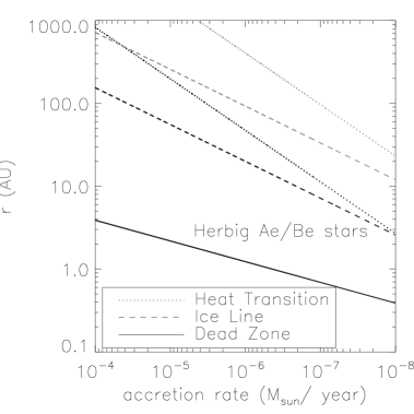
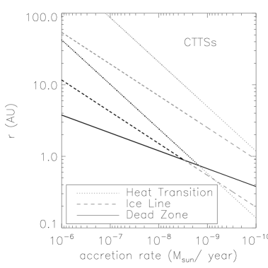
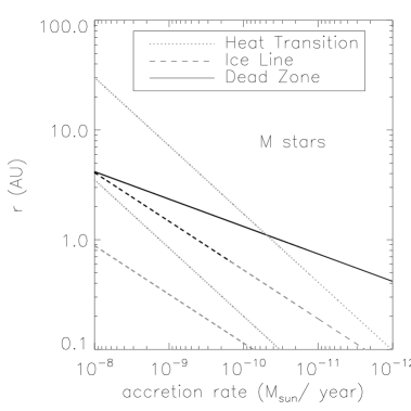
Figure 6: The location and evolution of all three planet traps. The heat transition traps with $\alpha=10^{-2}$ and $\alpha=10^{-5}$ are denoted by the lower and upper dotted lines, respectively (see equation (6)). The ice line traps with $\alpha=10^{-2}$ and $\alpha=10^{-5}$ are denoted by the lower and upper dashed lines, respectively (see equation (6.1)). The dead zone traps are shown by the solid line (see equation (6.3)). Taking into account their active conditions (see Table 8), all effective traps are denoted by the black lines. For the Herbig Ae/Be star case, all three traps are effective for a wide range of $\dot{M}$. For the CTTS case, the ice line and heat transition traps merge with the dead zone trap. For the M star case, the ice line trap disappear for low values of $\dot{M}$ (see equation (4.42)). Thus, planet traps interact with each other, depending on the stellar and disc parameters.

6.1 A picture of forming planetary systems around stars with various masses

Table 9: The position of planet traps

	Herbig Ae/Be stars
	$r_{edge}$ (AU)	$r_{il}$ (AU)	$r_{ht}$ (AU)
$\dot{M}=10^{-4}$($M_{\odot}$/year)	3.9	155	830
$\dot{M}=10^{-6}$($M_{\odot}$/year)	1.2	20	47
	CTTSs
	$r_{edge}$ (AU)	$r_{il}$ (AU)	$r_{ht}$ (AU)
$\dot{M}=10^{-6}$($M_{\odot}$/year)	3.7	11.7	42.4
$\dot{M}=10^{-8}$($M_{\odot}$/year)	1.2	1.5	2.4
	M stars
	$r_{edge}$ (AU)	$r_{il}$ (AU)	$r_{ht}$ (AU)
$\dot{M}=10^{-8}$($M_{\odot}$/year)	4.2	N/A	N/A
$\dot{M}=10^{-9}$($M_{\odot}$/year)	2.3	1.5	N/A

We present a picture of how planetary systems are established based on planet traps and discuss how host stars affect the size of planetary systems formed around them.

6.1.1 General picture

Fig. 7 schematically illustrates this. The disc radius of each planet trap comes from Fig. 6 for the case of CTTSs (also see Table 9). The structure of surface density is plotted based on our disc models discussed in $\S$ 4.4. Since we do not model the time dependency of $\dot{M}$ that gives the realistic value of surface density, we simply adopt the values of $\Sigma_{0}$ and $10^{2}\times\Sigma_{0}$ in Table 3 at $\dot{M}=10^{-8}M_{\odot}/year$ and $\dot{M}=10^{-6}M_{\odot}/year$, respectively. These choices do not affect our picture.

At the early stage of disc evolution ($\dot{M}=10^{-6}M_{\odot}/year$), the mass of protoplanets (denoted by the size of dots) which are captured in each trap is small, and they are widely separated. As the disc accretes onto the host star, the surface density of gas and the accretion rate decrease, and the position of the planet trap region with protoplanets captured moves inwards. Concurrently, the growth of these protoplanets proceeds. Since the rate at which each planet trap moves differs (see Table 9), the separations between these trapped planets shrink. Also, the solid surface density in each planet trap probably varies in accordance with the variation of the surface density of gas. Therefore, the growth rate at the dead zones and ice lines may be higher than that at the heat transition. At some point, the gravitational interaction between trapped planets could exceed planetary migration and planet-planet scattering effects begin to dominate. We leave the later stage of evolution of planetary systems into our forthcoming paper. However, we can speculate how planetary systems evolve as follows.

If the trapped (proto)planets distribute themselves closely enough, the most massive planet can surely survive the planet-planet interaction. On the other hand, the other two trapped planets could scatter inwards or outwards, or could be ejected from the system, depending on the mass of the most massive planet. Thus, our picture can in principle predict how planetary systems are formed, and what differentiates the formation of multiple planets versus single planet in a system.

6.1.2 Dependence on stellar masses and accretion rates

We discuss the effects of stellar masses and accretion rates on the scale of planetary systems based on our picture. Table 9 summarises the position of each planet traps at two different values of $\dot{M}$ for stars with various masses in Fig. 6. One immediately observes that the scale of orbital radii of planets captured in planet traps is a function of stellar masses and disc accretion rates. For Herbig Ae/Be stars, planetary systems can extend from the order of au to $\sim 10^{3}$ au. For CTTSs, the size of planetary systems shrinks to $\sim$ 10 au. For M stars, planetary systems may be well confined within a few au. We discuss more on the dependence on the stellar mass by comparing with the observations below.

Figure 7: Our general picture of the formation of planetary systems. The disc radius of each planet trap comes from Fig. 6 for the case of CTTSs. The position of each planet trap is summarised in Table 9. The structure of surface density is based on our disc model discussed in $\S$ 4.4. The dots denotes trapped protoplanets, and their size represents their masses. At the early stage of disc evolution (on the left panel), the accretion rate and the surface density are higher, and the separation between protoplanets which are captured at each trap is larger. Planetary masses are smaller. At the later stage of disc evolution (on the right panel), the accretion rate and the surface density become lower, and the separation becomes smaller. The planetary masses are now much larger. We assume that solid density at the outer edge of dead zones and ice lines is larger than that at the heat transition, based on the higher surface density of gas. It well illustrates how the orbital movement of planet traps at different rates affects the formation of planetary systems.

6.2 Implications for observations

We discuss the validity of our picture by comparing with the observations. Fig. 6 shows that the location of the dead zone traps for all cases is on order of 1 au (see the CTTS case). This is in accord with the observations which show statistically that the most gas giants are found around 1 au (e.g. Wright et al., 2009). Therefore, our finding may imply that the dead zones play a significant role in the formation and location of these planets.

For the case of Herbig Ae/Be stars (the top panel), there are three traps for high accretion rates. It is interesting that the range of disc radii for the heat transition and ice line traps covers the (large) range of orbital radii ($\sim 10^{2}-10^{3}$ au) of massive planets around massive stars such as A stars which are observed by the direct imaging method (e.g. Marois et al., 2008). For a lower accretion rate, the heat transition and ice line traps merge. However, the position of this merger is well separated from that of the dead zone trap. Thus, at least two planets may survive the planet-planet interaction. This multiplicity trend for massive stars is confirmed again by the direct imaging method (although the detected semi-major axes are considerably larger than our prediction.)

For the CTTSs case (the middle panel), three traps exist at first, and then as the disc accretion rate drops, the ice line and heat transition traps merge into the dead zone traps. As mentioned above, the interaction of three active traps arises around 1 au. Based on our picture, planets in multiple systems are less massive than single systems, since more massive planets provide more destructive effects on planetary systems. This prediction well explains the observation trend that (apparently) single planets statistically have larger masses than planets in multiple systems (Wright et al., 2009). More recently, the Kepler mission also confirmed the same trend (Latham et al., 2011). Thus, the interaction of planets in their traps is essential for a systematic understanding of how planetary systems are formed.

For the case of M stars (the bottom panel), only the dead zone trap is active at first. The location of this trap can explain the observed Super-Earth around M stars (Beaulieu et al., 2006). As the accretion rate decreases, the ice line trap appears and then disappears due to the constraint derived from equation (4.42) (see Table 8). In this case, it is more sensitive to when and what mass of planets are captured at each trap.

6.3 Parameter study

We perform a parameter study on $s_{A}$, $t$, and $\Sigma_{A0}$ (see Fig. 8). We adopt the values of the CTTSs case. Fig. 8 shows all the possible cases. The locations of $r_{il}$ and $r_{ht}$ are the same on all panels (since they are independent of these parameters, see equations (6.1) and (6)). The position of $r_{edge}$ is scaled by $\Sigma_{A0}$ while the dependence of $\dot{M}$ on $r_{edge}$ is controlled by the sum of $s_{A}$ and $t$ (see equation (6.3)). One immediately observes that the presence of multiple traps in a single disc is more likely than only a single planet trap over a wide range of $\dot{M}$. Hence, the interaction of planets which are growing and lodged in their traps can be considered as essential. As discussed above, the growth rate of trapped protoplanets which controls when the planet-planet interaction initiates is crucial. We will address this issue in the forthcoming paper, by taking into account the growth of protoplanet as well as disc evolution.

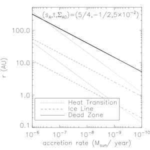
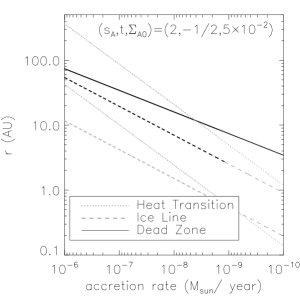
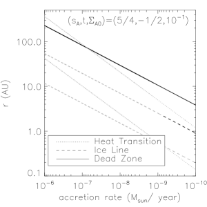
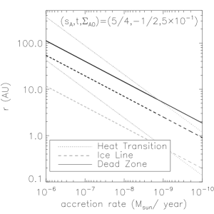
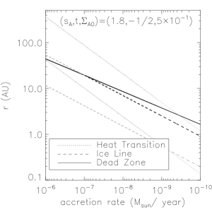
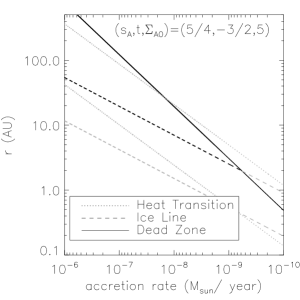
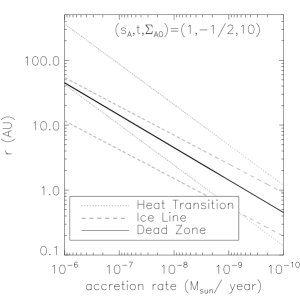
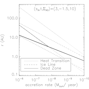
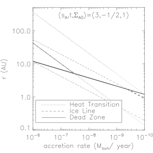
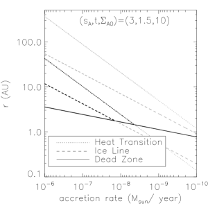
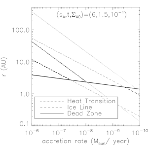
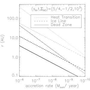
Figure 8: Parameter study on the location and evolution of three planet traps around CTTSs. The definitions of all lines are the same as Fig. 6. All possible cases are shown. Our choices of parameters are shown in each panel. The presence of multiple planet traps in a single disc is more common. Therefore, the interaction of the planet traps is likely essential.

7 Application to our Solar system

In this section, we apply our picture to the origin of the Solar system - in particular to the Nice model as developed by Tsiganis et al. (2005); Morbidelli et al. (2005); Gomes et al. (2005). In this model, the dynamics of outer planets is investigated by simulating planetary migration in a debris disc and the subsequent planet-planet interaction. Thus, the model assumes that all gas in the disc is depleted and planetary migration is caused by interactions with planetesimals. However, these N-body based simulations depend on their initial conditions which are not justified. More recently, Matsumura et al. (2010) investigated planetary migration in dissipating gaseous discs and showed that the semi-major axes are established by planetary migration in gaseous discs. Once gas is depleted, other orbital quantities such as eccentricities are determined by the planet-planet interaction. Therefore, it is crucial to examine the initial conditions of the Nice model in discs where gas is still present, in order to validate their results.

Fig. 9 shows the most plausible case for the initial condition of the Nice model in which Jupiter is placed at 5.45 au while Saturn at $\sim$ 8.2 au. We find it by varying the parameters ($s_{A},t,\Sigma_{A0}$). In this figure, we show the two expected traps: the ice line and dead zone traps. These two planet traps may be the building sites of the two gas giants (Jupiter and Saturn). The formation of the icy giants (Uranus and Neptune) may originate from scattering processes (Thommes et al., 1999). This idea is also supported by the Nice model. Thus, the core of the assumption in the Nice model is the initial semi-major axes of two gas giants (Jupiter and Saturn; see the horizontal solid lines). Fig. 9 indicates that these two traps deliver the cores of two gas giants to the initial semi-major axes for the Nice model towards the end of the gas disc’s lifetime, when the gas accretion rate have fallen to $\dot{M}=5.5\times 10^{-9}M_{\odot}/year$ (see the vertical solid line). At this moment, the disc still have considerable amount of gas ($\sim$ 1 per cent of $\Sigma_{0}$), and hence the initial condition adopted in the Nice model may be too simplified.

Another interesting point is that Jupiter hovers around the ice line trap (see Fig. 9). Since the dust density there is significantly enhanced, the formation of the trapped core of Jupiter speeds up considerably. This may be a reason why the mass of Jupiter is larger than that of Saturn. Recently, the significant improvements of the Nice model were achieved by incorporating planetary migration driven by the gas discs (Morbidelli, 2010, references herein). These studies showed that a key is the mass ratio of Jupiter to Saturn. If Jupiter is more massive than Saturn, the initial conditions adopted in the original Nice model are readily achieved. This is possible if there is outward migration of these two gas giants, which according to the model is consequence of capturing them into the 2/3 mean motion resonances (MMRs). If such a mass ratio of these two gas giants is not attained, both planets migrate inwards too rapidly to survive. Although these trends of migration happen without any planet trap, no one can currently explain such a mass ratio. Thus, our analyses are likely important for giving at least one explanation for deriving the initial conditions for the Nice model. We will address more comprehensive roles of planet traps in the Nice model in a future publication.

As the separation of these two traps decreases with decreasing accretion rates, the two trapped cores can induce scattering of any other cores formed around them. Thus, our approach is very useful to investigate the formation of planetary system more self-consistently. In the subsequent paper, we will include the growth of planets in viscously evolving discs.

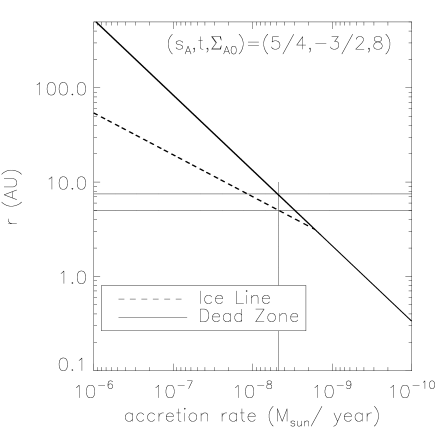
Figure 9: Application to the Nice model. Two planet traps exist in a single disc (as Fig. 6). The horizontal solid lines denote the initial condition of the semi-major axes for Jupiter ($r=5.45$ au, see the lower line) and Saturn ($r\approx$ 8.2 au, see the upper line), respectively in the Nice model. The core of Jupiter is captured at the ice line trap while that of Saturn is at the dead zone trap. At $\dot{M}=5.5\times 10^{-9}M_{\odot}/year$, the trapped cores reach the initial condition adopted in the Nice model.

8 Conclusions

We have systematically investigated how inhomogeneities arise in protoplanetary discs and how they create planet traps where the direction of planetary migration changes sign: from inwards to outwards. We analytically investigate the various mechanisms of planet traps activated by both corotation and Lindblad torques. For the traps related to the corotation torque, we have simply examined the disc structures that lead to outward migration. For the traps related to the Lindblad torque, we have derived the relations which predict when the torque reversal occurs.

Our analytical relations derived from the Lindblad torque succeed in reproducing the results of the previous numerical studies done for the dead zones: the density and thermal barriers ($\S$ 4.3). This confirms that our assumptions and treatments are valid for capturing the detailed, complex physics occurring in the simulations. Furthermore, we have shown that the ice lines can serve as barriers due to the Lindblad rather than corotation torque. In discs with MRI induced turbulence, the ice lines create the layered structure, so that the strength of turbulence ($\alpha$) reduces to the value of the dead zones. Thus, the ice lines can be considered to be self-regulated, localised dead zones. We have also discussed the possibility that a single disc can have several ice line barriers which become effective due to different species such as water-ice and CO-ice. A more detailed understanding of the structure of ice lines is required for addressing these features. Finally, we have estimated the mass range over which our analyses can apply. In either laminar or turbulent discs, our modeling can be useful for understanding almost observed exoplanets.

We summarise our major findings below.

1. We have shown that the heat transition of protoplanetary discs from viscosity to stellar irradiation dominated heating, activates a new barrier, which we call the heat transition barrier (see $\S$ 3.2.3). This barrier arises due to the entropy-related horseshoe drag and is caused by the temperature transition there. At disc radii inside the heat transition radius, $r_{ht}$, the temperature slope determined by viscous heating is very steep, resulting in outward migration. On the other hand, a shallower temperature profile controlled by stellar irradiation dominates at larger radii beyond $r_{ht}$. Such a region drives inward migration. Thus, planets which migrate toward the location of the heat transition are captured there.

2. We have also shown that a single disc can have up to three planet traps: the dead zone, ice line, and heat transition traps (see $\S$ 6). This multiplicity of planet traps is likely quite common. We have derived fully analytical relations for their disc radii and their effective conditions. These relations imply that dead zone traps may be the most important in order to explain why so many gas giants are observed around 1 au. Also, the presence of the heat transition and ice line traps may be the origin of massive planets with (very) large orbital radii around massive stars which are detected by the direct imaging method.

3. We have demonstrated that these planet traps can interact with each other, as they follow the time-dependent, viscous evolution of the disc (see Fig. 6). More specifically, we have found that their characteristic radii evolve with different dependence on $\dot{M}$ as the disc accretion rate $\dot{M}$ drops. This result shows that different planet traps move inwards differently, as discs accrete onto the central stars and star formation is terminated. (Equivalently, this evolution results in decreasing the surface density of gas ($\Sigma_{0}$) and accretion rates ($\dot{M}$).) Our analyses are important for comprehensively understanding the formation of planetary systems around stars with various masses (see Fig. 7). Since trapped planets can grow quickly, the interaction of active traps can initiate planet-planet interaction, which is controlled by the most massive, trapped planet. Thus, it is important to investigate how trapped planets gain their masses in viscously evolving discs. We will address this issue in a forthcoming paper.

4. We have applied our results to planet traps in discs around massive (Herbig Ae/Be), intermediate (CTTS), and low (M) mass stars. In all cases, the heat transition trap is the outermost trap in the disc while the dead zone or the ice line trap is the innermost. At low accretion rates ($\dot{M}\sim 10^{-8}M_{\odot}/year$) in CTTS system as an example, the traps are located at $r_{edge}=1.2$ au, $r_{il}=1.5$ au, and $r_{ht}=2.4$ au, respectively (see Table 9).

5. We have shown that the position of planet traps strongly depends on stellar masses and disc accretion rates. This indicates that host stars dictate a preferred scale of planetary systems formed around them (see Table 9). For Herbig Ae/Be stars, the size of planetary systems may expand from the order of a few au to $\sim 10^{3}$ au. For CTTSs, it shrinks to a few ten au. For M stars, any planetary systems formed around them may be well confined within the order of au.

6. We have applied our analyses to the Nice model for Solar system evolution. By choosing the appropriate parameters ($s_{A},t,\Sigma_{A0}$), we have shown that the ice line trap can capture the core of Jupiter while the dead zone trap Saturn. The locations of these trapped cores match those of the Nice model at $\dot{M}=5.5\times 10^{-9}M_{\odot}/year$ which is achieved towards the end of disc evolution. Furthermore, our analyses suggest why Jupiter is more massive than Saturn, which is one of the most crucial assumptions adopted in the improved Nice model.

In a subsequent paper, we will investigate the growth of planets which are captured at the planet traps during the time-dependent, viscous evolution of the disc. Inclusion of planetary growth will allow us to address when the planet-planet interaction dominates planetary migration.

Appendix A Extension of Paardekooper’s torque formula

Here, we discuss the extension of Paardekooper’s torque formula that is valid exclusively in pure power-law discs (see equation (3.2)). Since entropy gradients that scale an entropy-related corotation torque can be straightforwardly obtained from the disc profiles, we focus on the extension of Lindbald and vortensity-related corotation torques. For disc models, we adopt the same one in $\S$ 3.1, that is, general profiles for the surface density (see equation (3.1) ) and power-law profiles for the disc temperature ($T\propto r^{t}$). We only examine the case of $s=-1$ for $\Sigma_{int}$ (see equation (3.1)), because the results for the MMSN case are qualitatively similar. We also discuss the effects of the disc temperature that has more general profiles.

For the Lindblad torque, we indeed derive an analytical relation that controls the direction of migration for the above disc model in $\S$ 4.3 (see equation (4.20)). Exploiting the analysis, we estimate the critical value of $F_{g,crit}$ above which the Lindblad torque dictates outward migration:

$$F_{g,crit}\equiv\frac{\tanh(1/c)+h_{p}(s-t/2+7/4)}{\tanh(1/c)-h_{p}(s-t/2+7/4)},$$ (A.1)

where $h_{p}$ is the disc aspect ratio ($H/r$) at the position of a planet (see $\S$ 4.3.2 for a full derivation). Adopting $h_{p}=0.1$, we find that $F_{g,crit}=1.5$ for $c=1$ while $F_{g,crit}=2.7$ for $c=3$. As discussed in $\S$ 4.3.2, the direction of migration is determined only by the Lindblad torque if the density modification is larger than $F_{g,crit}$. This is because the Lindblad resonances distribute much further way from a planet than the horseshoe region. Based on the results of MG04 (see their fig. 1), the density distortion that is produced by the opacity and heat transitions is likely less than $F_{g,crit}$. In the following discussion, we adopt these critical values of $F_{g,crit}$. Thus, Lindblad torques surely become weaker around the opacity and heat transitions, but never give the dominant contribution to the direction of migration. Therefore, we adopt the original term derived in Paardekooper et al. (2010) for consistency in the usage of the torque formulation.

For the vortensity-related corotation torque, we add a correction factor $\phi_{v}$ in the original formulation (see equations (3.5) and (3.3)). This is because gradients of vortensity that are the core of the vortensity-related corotation torque, are very sensitive to the disc structure. Fig. 10 shows the surface density structure, the resultant behaviour of $\phi_{v}$, and the critical value of $t$ below which planets migrate outwards (see equation (3.5)) on the top, middle, and bottom panel, respectively. Since the vortensity gradients depend on the disc temperature through $\Omega$ (see equations (3.4) and (4.3)), self-consistent treatments are required to derive $t$. For simplicity, however, we fix $t=-1.2$ for determining $\phi_{v}$ in this figure. This profile is established for viscously heated, optically thick discs (see $\S$ 3.2.2). We also discuss the effects of the disc temperature with more general profiles below.

Fig. 10 shows very complicated behaviour for $\phi_{v}$. It is obvious that the choice of $c=1$ (the solid line) is more appropriate for the opacity and heat transitions based on the results of MG04. However, we also consider $c=3$ (the dashed line) for a parameter study. By comparing the middle and bottom panels, one can observe immediately that the crucial effects of $\phi_{v}$ on $t$ arise from Gaussian-like functions that distribute around $r_{trans}$. It is important that the extent of the functions is well characterised by the transition width ($\omega=cH$) (see the vertical lines on the bottom panel). For the case of $c=3$, the function expands beyond the transition width. However, this is a result of our choice of the temperature profile. Adopting more general profiles similar to equation (3.1) for the disc temperature, the extent of this function strongly diminishes (see Fig. 11). Thus, it is reasonable to conclude that the effects of $\phi_{v}$ are very local and well confined with the transition width. Another important point is that the required value of $t$ is strongly reduced by $\phi_{v}$. Such small values of $t$ are never accomplished in protoplanetary discs. This means that the vortensity-related corotation torque becomes significantly large and results in inward migration. Therefore, inclusion of $\phi_{v}$ reduces the possible outward migration region which is a consequence of viscous heating and entropy-related corotation torques.

In summary, proper treatments of the vortensity-related corotation torque are important for discs with general profiles. However, the deviation from the power-law treatments is well confined in the vicinity of the position of disc inhomogeneities, and therefore power-law approximation provides reliable results in our level of extension.

Figure 10: The structure of the vortensity correction factor $\phi_{v}$ for discs with general profiles. On the top panel, the surface density structures are plotted (see equation (3.1)). On the middle, the resultant behaviours of $\phi_{v}$ are shown. On the bottom, the critical values of $t$ affected by $\phi_{v}$ are plotted. We stress that the choice of $c=1$ is more appropriate for opacity and heat transitions. For the purpose of a parameter study, we also consider $c=3$. The results of pure power-law discs are denoted by the horizontal lines on the middle and bottom panels. The crucial effects of $\phi_{v}$ arise from Gaussian-like functions that are well confined with the transition width $(\omega=cH)$ (also see Fig. 11). Inclusion of $\phi_{v}$ significantly lowers the required value of $t$ around $r=r_{trans}$. This indicates that the vortensity-related corotation torque becomes considerably larger there and makes planets migrate inwards. Thus, proper treatments of the vortensity-related corotation torque deviates the results of the pure power-law discs, but the deviations occur only in the local region centered at $r=r_{trans}$.

Figure 11: The critical value of $t$ for the disc temperature with general profiles. We adopt an expression similar to equation (3.1) for the disc temperature. Also, we consider the case of $c=1$. By comparing Fig. 10, the extent wherein $\phi_{v}$ plays a crucial role is strongly diminished. This supports the usage of the pure power-law approximation.

Appendix B Taylor expansion of the tidal torque

Here, we derive the Taylor expansion of quantities related with the tidal torque in terms of $1/m\ll 1$ since the torque takes the maximum value at the wavenumber $m\approx 10$ (Ward, 1997).

$$\frac{\Sigma}{H}\cdot\alpha_{r}^{2} = \frac{\Sigma}{H}(r_{p})\alpha_{r}^{s-t/2+1/2}$$ (B.1)

$$\approx \frac{\Sigma}{H}(r_{p})\left[1+\frac{2\epsilon}{3m}\sqrt{1+\xi^{2}}\left(s-\frac{t}{2}+\frac{1}{2}\right)\right],$$

and

$$\psi \approx \left[K_{1}(\Lambda_{0})+2\sqrt{1+\xi^{2}}K_{0}(\Lambda_{0})\right]+$$ (B.2)

$$\frac{\epsilon}{m}\left[\left(\frac{5}{6}+\frac{2\xi^{2}}{3}\right)\sqrt{1+\xi^{2}}K_{1}(\Lambda_{0})+\left(\frac{1}{6}-\frac{\xi^{2}}{3}\right)K_{0}(\Lambda_{0})\right]$$

$$\equiv \psi_{0}+\frac{\epsilon}{m}\Delta\psi$$

with

$$\Lambda\approx\frac{2}{3}\sqrt{1+\xi^{2}}-\frac{\epsilon}{m}\frac{1+\xi^{2}}{3}\equiv\Lambda_{0}+\frac{\epsilon}{m}\Delta\Lambda,$$ (B.3)

and

$$K_{n}(z) = K_{n-2}(z)+\frac{2(n-1)}{z}K_{n-1}(z),$$ (B.4)

$$\frac{dK_{n}(z)}{dz} = -\frac{1}{2}\left(K_{n-1}(z)+K_{n+1}(z)\right).$$ (B.5)

Thus,

$$\psi^{2}\approx\psi_{0}^{2}[1+2(\epsilon/m)(\Delta\psi/\psi_{0})].$$ (B.6)

Taking the limit $\xi\rightarrow 0$ (since the effect of gas pressure becomes negligible in the Keplerian discs),

$$2\frac{\Delta\psi}{\psi_{0}}\approx\frac{1}{3}\frac{5K_{1}(2/3)+K_{0}(2/3)}{K_{1}(2/3)+2K_{0}(2/3)}\sim\frac{5}{6}.$$ (B.7)

Appendix C Ice lines of other molecules

Here, we investigate the minimum abundance of a molecule that is required for its ice line to be a barrier, by using the analyses done in $\S$ 4.4. Assuming the dust density to increase by the amount of ice which is formed at the ice line radius of a specific molecule, $r$, the required dust density enhancement is (using equations (4.35) and (4.27)), for $r/r_{edge}<$1,

$$f_{d1}>\frac{K_{1}-K_{2}}{K_{3}}=f(\alpha_{A},\alpha_{D},s_{A},t,h,r,f_{d2},c),$$ (C.1)

where

$$K_{1}=h_{p}\left(-\frac{3}{2}t+\frac{1}{4}\right)\frac{\alpha_{A}+\alpha_{D}}{\alpha_{A}-\alpha_{D}}\left(\frac{r_{edge}}{r}\right)^{s_{A}+t+3/2},$$ (C.2)

$$K_{2}=h\left[B\left(s_{A}-\frac{t}{2}+\frac{7}{4}\right)-(B-1)\frac{t+3}{c^{2}}\left(-\frac{t}{2}+\frac{7}{4}\right)\right],$$ (C.3)

and

$$K_{3}=\frac{\tanh(1/c)}{2}\left(B-(B-1)\frac{t+3}{c^{2}}\right)+\frac{K_{2}}{2},$$ (C.4)

For $r/r_{edge}>$1, the dust density enhancement needed is given as

$$g_{d}>\frac{-3t/2+1/4}{3t/2-1/4+\sqrt{\ln 2}/ch},$$ (C.5)

where equation (4.41) is used. In order to gain a unified condition for the entire of discs, we find the relation between $f_{d1}$ and $g_{d}$ which is given as

$$g_{d} = \frac{\alpha_{A}-\alpha_{D}}{\alpha_{D}}\left[1-\frac{\alpha_{A}}{\alpha_{A}+\alpha_{D}}\right.$$

$$\times \left.\left(\frac{r}{r_{edge}}\right)^{s_{A}+t+3/2}\left(1+\frac{f_{d1}}{2}\right)^{-1}\left(1+f_{d2}\right)^{-1}\right].$$

As a result, equation (C.5) becomes

$$f_{d1}>\frac{2(P_{1}+P_{2}-1)}{1-P_{2}},$$ (C.7)

where

$$P_{1}=\frac{\alpha_{A}}{\alpha_{A}+\alpha_{D}}\left(\frac{r}{r_{edge}}\right)^{s_{A}+t+3/2}\left(1+f_{d2}\right)^{-1},$$ (C.8)

and

$$P_{2}=\frac{\alpha_{D}}{\alpha_{A}-\alpha_{D}}\frac{-3t/2+1/4}{3t/2-1/4-\sqrt{\ln 2}/ch}.$$ (C.9)

Fig. 12 shows the threshold value of $f_{d1}$ as a function of $r/r_{edge}$. We define a fiducial model as ($s_{A},t,h_{edge},f_{d2},c$)=(3,-1/2,0.1,0,1). The required value of $f_{d1}$ are above the lines. We performed parameter studies on $h_{edge}$, $s_{A}$, and $t$ and the results are shown in the top, middle, and bottom panels, respectively.

For $r/r_{edge}<$1, the dominant term in equation (C.1) is $(r_{edge}/r)^{s_{A}+t+3/2}$ in $K_{1}$. We see that a large value of $f_{d1}$ is required for outward migration, if the value of $s_{A}+t+3/2$ is positive. Fig. 12 shows that small separations between the ice line and dead zone barriers are again preferred. If $s_{A}+t+3/2<$0, a tiny amount of ice is enough to provide a barrier (see the dashed line on the middle panel). This indicates that ice lines of relatively abundant molecules can work as barriers. For $r/r_{edge}>$1, the dominant term in equation (C.7) is $(r/r_{edge})^{s_{A}+t+3/2}$ in $P_{1}$. Consequently, a significantly large value of $f_{d1}$ is needed for outward migration, if the value of $s_{A}+t+3/2$ is positive. In fact, it may not be possible for ice lines of any molecule to be a barrier in this case. On the other hand, if $s_{A}+t+3/2$ is negative, the amount of ice does not matter. (see the dashed line on the middle panel). This implies that ice lines of any species can act as barriers. Thus, the required $f_{d1}$ strongly depends on the sum of $s_{A}$ and $t$.

What value of $s_{A}$ is most appropriate for realistic discs? For $r/r_{edge}<$1, $s_{A}$ should be positive. Otherwise, dead zones cannot exist. This indicates that larger values of $f_{d1}$ are required as $r/r_{edge}$ decreases, and hence only specific, abundant species in discs can work as a barrier. For $r/r_{edge}>$1, $s_{A}$ should be negative, since $\Sigma_{A}\approx\Sigma$. Thus, it is likely that the abundance of molecules may not be important for providing a barrier. As a result, several ice line barriers which are excited by different species such as water-ice and CO-ice may be present in a single disc. However, the value of $s_{A}$ strongly depends on how icy dust absorbs free electrons and how these distributions evolve with time.

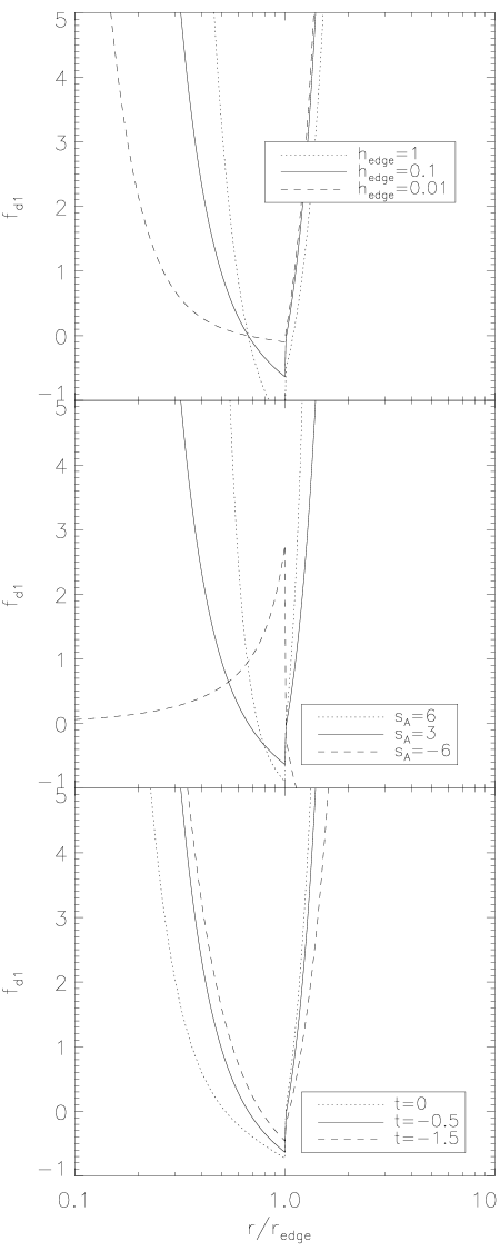
Figure 12: The enhancement $f_{d1}$ of the dust density required to produce ice line barriers. For $r/r_{edge}<$1, equation (C.1) is adopted while equation (C.7) is used for $r/r_{edge}>$1. We define a fiducial model as ($s_{A},t,h_{edge},f_{d2},c$)=(3,-1/2,0.1,0,1). We vary $h_{edge}$, $s_{A}$, and $t$ on the top, middle, and bottom panel, respectively. A large value of $f_{d1}$ is required for ice lines to be a barrier, if $s_{A}+t+3/2$ is positive. On the other hand, the presence of ice line barriers becomes insensitive to $f_{d1}$ if $s_{A}+t+3/2$ is negative (see the dashed line on the middle panel). It implies that the minimum value of $f_{d1}$ strongly depends on the detail structure of ice lines.

References

- Adachi et al. (1976) Adachi I., Hayashi C., Nakazawa K., 1976, Prog. Theor. Phys., 56, 1756
- Adams et al. (1987) Adams F. C., Lada C. J., Shu F. H., 1987, ApJ, 312, 788
- Aikawa & Herbst (1999) Aikawa Y., Herbst E., 1999, A&A, 351, 233
- Alibert et al. (2005) Alibert Y., Mordasini C., Benz W., Winisdoerffer C., 2005, A&A, 434, 343
- Artymowicz (1993) Artymowicz P., 1993, ApJ, 419, 155
- Bai & Stone (2010) Bai X.-N., Stone J. M., 2010, ApJ, 722, 1437
- Basset (1998) Basset B., 1998, Comput. Math. Applic., 36, 37
- Beaulieu et al. (2006) Beaulieu J.-P., et al., 2006, Nat, 439, 437
- Bell & Lin (1994) Bell K. R., Lin D. N. C., 1994, ApJ, 427, 987
- Chiang & Youdin (2010) Chiang E., Youdin A. N., 2010, AREPS, 38, 493
- Chiang & Goldreich (1997) Chiang E. I., Goldreich P., 1997, ApJ, 490, 368
- D’Alessio et al. (1998) D’Alessio P., Cantó J., Calvet N., Lizano S., 1998, ApJ, 500, 411
- Davis (2005) Davis S. S., 2005, ApJ, 620, 994
- Davis (2007) Davis S. S., 2007, ApJ, 660, 1580
- Dullemond et al. (2007) Dullemond C. P., Hollenbach D., Kamp I., D’Alessio P., 2007, Protostars and Planets V. Univ. Arizona Press, Tucson
- Ford & Rasio (2008) Ford E. B., Rasio F. A., 2008, ApJ, 686, 621
- Gammie (1996) Gammie C. F., 1996, ApJ, 457, 355
- Goldreich & Tremaine (1980) Goldreich P., Tremaine S., 1980, ApJ, 241, 425
- Gomes et al. (2005) Gomes R., Levison H. F., Tsiganis K., Morbidelli A., 2005, Nat, 435, 466
- Gorti & Hollenbach (2009) Gorti U., Hollenbach D., 2009, ApJ, 690, 1539
- Hasegawa & Pudritz (2010a) Hasegawa Y., Pudritz R. E., 2010a, ApJ, 710, L167
- Hasegawa & Pudritz (2010b) Hasegawa Y., Pudritz R. E., 2010b, MNRAS, 401, 143
- Hasegawa & Pudritz (2011) Hasegawa Y., Pudritz R. E., 2011, MNRAS, 413, 286
- Hollenbach et al. (1994) Hollenbach D., Johnstone D., Lizano S., Shu F., 1994, ApJ, 428, 654
- Howard et al. (2011) Howard A. W., et al., 2011, ApJ, submitted (astro-ph/arXiv:1103.2541v1)
- Hubeny (1990) Hubeny I., 1990, ApJ, 351, 632
- Ida & Lin (2008) Ida S., Lin D. N. C., 2008, ApJ, 685, 584
- Ilgner & Nelson (2006) Ilgner M., Nelson R. P., 2006, A&A, 445, 205
- Jang-Condell & Sasselov (2004) Jang-Condell H., Sasselov D. D., 2004, ApJ, 608, 497
- Jang-Condell & Sasselov (2005) Jang-Condell H., Sasselov D. D., 2005, ApJ, 619, 1123
- Johnstone et al. (1998) Johnstone D., Hollenbach D., Bally J., 1998, ApJ, 499, 758
- Kenyon & Hartmann (1987) Kenyon S. J., Hartmann L., 1987, ApJ, 323, 714
- Kley & Crida (2008) Kley W., Crida A., 2008, A&A, 487, L9
- Kokubo & Ida (2000) Kokubo E., Ida S., 2000, Icarus, 143, 15
- Kretke & Lin (2007) Kretke K. A., Lin D. N. C., 2007, ApJ, 664, L55
- Latham et al. (2011) Latham D. W., et al., 2011, ApJL, submitted (astro-ph/arXiv:1103.3896v1)
- Lubow & Ogilvie (1998) Lubow S. H., Ogilvie G. I., 1998, ApJ, 504, 983
- Lynden-Bell & Pringle (1974) Lynden-Bell D., Pringle J. E., 1974, MNRAS, 168, 603
- Lyra et al. (2010) Lyra W., Paardekooper S.-J., Mac Low M.-M., 2010, ApJ, 715, L68
- Marois et al. (2008) Marois C., Macintosh B., Barman T., Zuckerman B., Song I., Patience J., Lafrenière D., Doyon R., 2008, Sci, 322, 1348
- Masset & Casoli (2010) Masset F. S., Casoli J., 2010, ApJ, 723, 1393
- Masset et al. (2006) Masset F. S., Morbidelli A., Crida A., Ferreira J., 2006, ApJ, 642, 478
- Matsumura & Pudritz (2006) Matsumura S., Pudritz R. E., 2006, MNRAS, 365, 572
- Matsumura et al. (2007) Matsumura S., Pudritz R. E., Thommes E. W., 2007, ApJ, 660, 1609
- Matsumura et al. (2009) Matsumura S., Pudritz R. E., Thommes E. W., 2009, ApJ, 691, 1764
- Matsumura et al. (2010) Matsumura S., Thommes E. W., Chatterjee S., Rasio F. A., 2010, ApJ, 714, 194
- Menou & Goodman (2004) Menou K., Goodman J., 2004, ApJ, 606, 520
- Min et al. (2011) Min M., Dullemond C. P., Kama M., Dominik C., 2011, Icarus, 212, 416
- Morbidelli (2010) Morbidelli A., 2010, C. R. Physique, 11, 651
- Morbidelli et al. (2008) Morbidelli A., Crida A., Masset F., Nelson R. P., 2008, A&A, 478, 929
- Morbidelli et al. (2005) Morbidelli A., Levison H. F., Tsiganis K., Gomes R., 2005, Nat, 435, 462
- Mordasini et al. (2009) Mordasini C., Alibert Y., Benz W., 2009, A&A, 501, 1139
- Mordasini et al. (2011) Mordasini C., Dittkrist K.-M., Alibert Y., Klahr H., Benz W., Henning T., 2011, preprint (astro-ph/arXiv:1101.3238v1)
- Nakamoto & Nakagawa (1994) Nakamoto T., Nakagawa Y., 1994, ApJ, 421, 640
- Nelson & Gressel (2010) Nelson R. P., Gressel O., 2010, MNRAS, 409, 639
- Paardekooper et al. (2010) Paardekooper S.-J., Baruteau C., Crida A., Kley W., 2010, MNRAS, 401, 1950
- Paardekooper et al. (2011) Paardekooper S.-J., Baruteau C., Kley W., 2011, MNRAS, 410, 293
- Paardekooper & Mellema (2006) Paardekooper S.-J., Mellema G., 2006, A&A, 459, L17
- Paardekooper & Papaloizou (2009) Paardekooper S.-J., Papaloizou J. C. B., 2009, MNRAS, 394, 2283
- Rasio & Ford (1996) Rasio F. A., Ford E. B., 1996, Sci, 274, 954
- Ruden & Lin (1986) Ruden S. P., Lin D. N. C., 1986, ApJ, 308, 883
- Sándor et al. (2011) Sándor Z., Lyra W., Dullemond C. P., 2011, ApJ, 728, 9L
- Sano et al. (2000) Sano T., Miyama S., Umebayashi T., Nakano T., 2000, ApJ, 543, 486
- Shakura & Sunyaev (1973) Shakura N. I., Sunyaev R. A., 1973, A&A, 24, 337
- Tanaka et al. (2002) Tanaka H., Takeuchi T., Ward W. R., 2002, ApJ, 565, 1257
- Thommes et al. (1999) Thommes E. W., Duncan M. J., Levison H. F., 1999, Nat, 402, 635
- Thommes et al. (2008) Thommes E. W., Matsumura S., Rasio F. A., 2008, Sci, 321, 814
- Tsiganis et al. (2005) Tsiganis K., Gomes R., Morbidelli A., Levison H. F., 2005, Nat, 435, 459
- Ward (1988) Ward W. R., 1988, Icarus, 73, 330
- Ward (1997) Ward W. R., 1997, Icarus, 126, 261
- Weidenschilling (1977) Weidenschilling S. J., 1977, MNRAS, 180, 57
- Wright et al. (2009) Wright J. T., Upadhyay S., Marcy G. W., Fischer D. A., Ford E. B., Johnson J. A., 2009, ApJ, 693, 1084
- Yang & Menou (2010) Yang C.-C., Menou K., 2010, MNRAS, 402, 2436