Photometric redshifts and quasar probabilities from a single, data-driven generative model

Abstract

We describe a technique for simultaneously classifying and estimating the redshift of quasars. It can separate quasars from stars in arbitrary redshift ranges, estimate full posterior distribution functions for the redshift, and naturally incorporate flux uncertainties, missing data, and multi-wavelength photometry. We build models of quasars in flux–redshift space by applying the extreme deconvolution technique to estimate the underlying density. By integrating this density over redshift one can obtain quasar flux–densities in different redshift ranges. This approach allows for efficient, consistent, and fast classification and photometric redshift estimation. This is achieved by combining the speed obtained by choosing simple analytical forms as the basis of our density model with the flexibility of non-parametric models through the use of many simple components with many parameters. We show that this technique is competitive with the best photometric quasar classification techniques—which are limited to fixed, broad redshift ranges and high signal-to-noise ratio data—and with the best photometric redshift techniques when applied to broadband optical data. We demonstrate that the inclusion of UV and NIR data significantly improves photometric quasar–star separation and essentially resolves all of the redshift degeneracies for quasars inherent to the $ugriz$ filter system, even when included data have a low signal-to-noise ratio. For quasars spectroscopically confirmed by the SDSS 84 and 97 percent of the objects with GALEX UV and UKIDSS NIR data have photometric redshifts within 0.1 and 0.3, respectively, of the spectroscopic redshift; this amounts to about a factor of three improvement over $ugriz$-only photometric redshifts. Our code to calculate quasar probabilities and redshift probability distributions is publicly available.

Section 1 Introduction

The last decade has seen the first instances of statistical studies with quasars using purely photometric samples. Examples of these include the measurement of the integrated Sachs–Wolfe effect (Giannantonio et al., 2006, 2008) and cosmic magnification bias (Scranton et al., 2005a), and studies of the clustering of quasars on large (Myers et al., 2006, 2007a) and small (Hennawi et al., 2006a; Myers et al., 2007b) scales. The importance of photometrically classified quasar samples will only increase during the next decade as large new imaging surveys will uncover large samples of quasars at fainter magnitudes, with minimal spectroscopy for the faintest objects. While efficient photometric classification is one requirement to facilitate studies of quasars without extensive spectroscopy, it has also been crucial to develop accurate methods for quasar redshift estimation based on broadband photometry. Techniques for photometric redshift estimation have long been successful for galaxies (e.g., Baum, 1962; Connolly et al., 1995) and became feasible for quasars with the advent of precise multi-filter photometry (Richards et al., 2001a, b; Budavári et al., 2001; Wolf et al., 2004).

Closely related to the quasar photometric-redshift problem—traditionally seen as a regression problem—is the question as to how best to perform photometric classification of quasars. It has become clear that the best classifiers are probabilistic in nature in that they calculate probabilities for objects to be quasars based on accurately calibrated models for stellar and quasar photometry (e.g., Richards et al., 2004; Bovy et al., 2011). These probabilities are often calculated for quasars in certain broad redshift ranges, and they therefore also act as low-resolution photometric redshifts for the objects they classify as quasars. The object classification technique of Suchkov et al. (2005) uses bins of width $\Delta z=0.2$ and, thus, achieves classification with a finer photometric-redshift estimate. However, detailed photometric redshift estimates for photometrically classified quasars utilize heterogeneous techniques, such that the resulting redshift probability distributions are inconsistent with the broad probabilities used for the initial quasar classification. For instance, this is the case for the photometric quasar catalogs of Richards et al. (2004, 2009a). For these catalogs, a non-parametric kernel-density-estimation (KDE) technique that ignores photometric uncertainties was used to classify quasars, while a parametric model that convolves the quasar color locus with the photometric uncertainties—a single Gaussian distribution in bins of redshift $\Delta z\approx 0.075$—was applied to estimate redshift (Weinstein et al., 2004).

For many purposes, one would like to target quasars in arbitrary redshift ranges that differ from those predetermined and imposed by a broad classification method. For example, the Baryon Oscillation Spectroscopic Survey (BOSS; Eisenstein et al. 2011) of The Sloan Digital Sky Survey III (SDSS-III) aims to measure the baryon acoustic feature in the Ly$\alpha$ forest of medium-redshift ($2.2\lesssim z\lesssim 4.0$) quasars (e.g., McDonald & Eisenstein, 2007; McQuinn & White, 2011). The spectral range accessible to the BOSS spectrographs is $3600<\lambda<10000$ Å (Barkhouser et al., 2011, in preparation), thus BOSS can only study the Ly$\alpha$ forest as traced by redshift $z\gtrsim 2.2$ quasars. Therefore, BOSS requires quasars to be targeted based on their probability to be at redshift $\geq 2.2$, and the BOSS quasar classifiers were trained with this constraint (e.g., Ross et al., 2011; Bovy et al., 2011). However, other ground-based instruments can observe at shorter wavelengths, e.g., the Multi-Object Double Spectrograph for the Large Binocular Telescope, which can observe the spectral range $3400\AA\ <\lambda<10000$ Å (Pogge et al., 2010). This instrument could study the Ly$\alpha$ forest starting at redshift $z\gtrsim 2$. An Ly$\alpha$ forest experiment designed for the Large Binocular Telescope might therefore target quasars in the redshift range $2.0\leq z<2.2$ in addition to those at higher redshift.

Another example of a project that requires accurate photometric characterization of quasars is the search for binary quasars (Hennawi et al., 2006a; Myers et al., 2008; Hennawi et al., 2010; Shen et al., 2010), where the key metric is the probability that two objects are both quasars and proximate in redshift, i.e., the joint (or “overlapping”) probability that both components of a pair of objects are quasars of a particular redshift. Similarly, the search for projected quasar pairs for absorption line studies (Hennawi et al., 2006b; Bowen et al., 2006; Hennawi & Prochaska, 2007; Prochaska & Hennawi, 2009) requires the joint probability that both objects in a projected pair are quasars. Such calculations require a full model of quasar probabilities and redshifts. Ideally, therefore, photometric redshift estimation and quasar classification ought to be performed together.

In the specific case of objects observed using the $ugriz$ filter system (Fukugita et al., 1996), quasar photometric redshifts are plagued by a host of degeneracies at redshifts where various quasar emission lines are mistaken for the Ly$\alpha$ line (Richards et al., 2002); this results in “catastrophic” redshift failures, although consideration of the full redshift posterior distribution function (PDF) shows that most of these failures have a significant integrated probability around the correct redshift (e.g., Ball et al. 2008; see below). The addition of non-$ugriz$ data, e.g., ultraviolet (UV) and near-infrared (NIR) measurements, can both alleviate these redshift degeneracies and improve quasar–star separation. Quasar classification and characterization in the infrared has been considered for simulated objects and for quasar samples with a range of depths and areas (e.g., Warren et al., 2000; Croom et al., 2001; Francis et al., 2004; Glikman et al., 2006; Maddox & Hewett, 2006; Chiu et al., 2007; Richards et al., 2009b; D’Abrusco et al., 2009; Assef et al., 2010; Wu & Jia, 2010; Peth et al., 2011). The NIR is also the region to search for the highest redshift quasars (redshift $z\gtrsim 6$; Mortlock et al., 2011). These studies show the great promise that NIR data hold for quasar selection and redshift estimation. The UV holds a similar potential (see, e.g., Atlee & Gould, 2007; Trammell et al., 2007; Jimenez et al., 2009; Hutchings & Bianchi, 2010).

The technique we introduce in this article, which we denote XDQSOz, is the first that deals with the simultaneous classification of quasars and assignation of quasar redshifts. This technique extends the XDQSO quasar classification technique of Bovy et al. (2011) to model the density of quasars in color–redshift space with a flexible semi-parametric model consisting of a large set of Gaussian component distributions. This model can be integrated analytically over any redshift range to calculate probabilities from flux measurements for individual objects. This, in turn, allows quasar probabilities to be calculated over any redshift range. Thus, a probability distribution in redshift space (a “PDF”) is a natural component of the model. Because we use the extreme deconvolution (XD) technique (Bovy et al., 2009) as our density estimation tool, the method can be trained on and applied to low signal-to-noise ratio data, even with missing values, e.g., to objects missing measurements in any arbitrary collection of filters. This feature allows us to naturally include UV and NIR broadband fluxes, where sky coverages differ, as part of our model space and to distinguish sources that are missing data in a particular band from objects that are dropping out of that band. We show that the addition of UV and NIR broadband fluxes improves quasar–star separation significantly and that it essentially breaks all of the redshift degeneracies inherent to the $ugriz$ filter set.

This article is organized as follows. In Section 2, we discuss general aspects of photometric redshift estimation and classification in the context of quasars. We briefly describe the data used to train and test the new method in Section 3. Section 4 contains a full description of the XDQSOz quasar model and Section 5 shows how this model is used to calculate quasar probabilities over arbitrary redshift ranges. Section 6 assesses the performance of the photometric redshifts obtained using the XDQSOz model. A discussion of various extensions of the model is given in Section 7 and we conclude in Section 8. The Appendix describes the photometric classification and redshift estimation XDQSOz code that is made publicly available.

In what follows, AB magnitudes (Oke & Gunn, 1983) are used throughout. Where dereddened fluxes and magnitudes are required we have used the reddening maps of Schlegel et al. (1998). All magnitudes and fluxes should be considered as dereddened unless mentioned otherwise.

Section 2 General considerations

A technique for photometric redshift estimation of quasars should have the following properties.

• It should provide full probability distributions for the redshift of the quasar based on its observed photometry, because this information has particular utility for quasars (e.g., Myers et al., 2009) as near-degeneracies in redshift estimation from broadband photometry are ubiquitous for quasars (e.g., Richards et al., 2001b; Budavári et al., 2001).

• Upon the evaluation of the probability of the redshift the photometric uncertainties should be treated properly to allow photometric redshift estimation for faint objects.

• If based on an empirical training set, the technique should be able to be trained on low signal-to-noise ratio data with potentially missing data. The training set and the evaluation set should also be allowed to have different noise properties, e.g., different distributions of signal-to-noise ratio. For example, while the optical fluxes are mostly well measured for a spectroscopic training sample, the addition of UV and NIR data can help break redshift degeneracies (see below), but these measurements often have low signal-to-noise ratio, even for the training set.

• The technique should allow an explicit redshift prior to be specified.

The key to photometric classification and redshift estimation for quasars based on broadband fluxes is the joint probability of an object’s fluxes, its redshift, and the proposition that it is a quasar $p(\mathrm{flux},z,\mathrm{quasar})$. This joint probability can be re-written in several ways that correspond to different ways of approaching the problem

$$p(\mathrm{fluxes},z,\mathrm{quasar}) =p(\mathrm{fluxes}|z,\mathrm{quasar})\,p(z|\mathrm{quasar})\,P(\mathrm{quasar})$$ (1)

$$=p(\mathrm{fluxes},z|\mathrm{quasar})\,P(\mathrm{quasar})$$ (2)

$$=p(z|\mathrm{fluxes},\mathrm{quasar})\,p(\mathrm{fluxes}|\mathrm{quasar})\,P(\mathrm{quasar})\,.$$ (3)

Photometric redshift estimation corresponds to the probability of an object’s redshift conditioned on its fluxes and assuming that it is a quasar:

$$p(z|\mathrm{fluxes},\mathrm{quasar})=\frac{p(\mathrm{fluxes},z,\mathrm{quasar})}{p(\mathrm{fluxes},\mathrm{quasar})}\,.$$ (4)

Quasar classification is the probability that an object is a quasar based on its fluxes. To classify quasars in a certain redshift range $\Delta z$, we integrate the joint probability that the object is a quasar with redshift $z$ over redshift:

$$P(\mathrm{quasar\ in}\ \Delta z|\mathrm{fluxes}) =\int_{\Delta z}\mathrm{d}z\,p(\mathrm{quasar},z|\mathrm{fluxes})$$ (5)

$$=\int_{\Delta z}\mathrm{d}z\,\frac{p(\mathrm{quasar},z,\mathrm{fluxes})}{p(\mathrm{fluxes})}$$ (6)

The probability that an object is a quasar of any redshift is obtained by setting the redshift range $\Delta z=[0,\infty]$. The normalization factor $p(\mathrm{fluxes})$ in this equation is given by

$$p(\mathrm{fluxes})=p(\mathrm{fluxes},\mathrm{quasar})+p(\mathrm{fluxes},\mathrm{not\ a\ quasar})\,.$$ (7)

The probability of an object not being a quasar can be obtained empirically by modeling the fluxes of non-quasars (see Richards et al., 2004; Bovy et al., 2011).

The discussion above suggests that a unified approach to classification and photometric redshift estimation is possible. Because the method described in this article is the first technique in this class, we briefly discuss previous attempts at photometric redshift estimation and how they fit in the framework outlined in this section.

The $k$-nearest neighbors approach of Ball et al. (2007) is an instance-based machine-learning technique that compares the colors of test objects to the $k$ nearest objects in color-space in a training set, and assigns a weighted combination of the redshifts of those nearest neighbors to the test object. Its generalization to take observational flux-uncertainties into account involves perturbing both the test and the training data within their Gaussian noise ellipsoids (Ball et al., 2008). In its noiseless implementation the method does not return a full probability distribution for the redshift. When taking the photometric uncertainties into account the technique essentially returns samples from $p(z|\mathrm{flux},\mathrm{quasar})$ as in equation (3), which can be binned to obtain the full posterior distribution function. While the photometric uncertainties of the test objects are handled correctly, the approach for dealing with the uncertainties of the training data effectively convolves with the uncertainties twice, as it adds scatter to the training data that are already scattered from the intrinsic distribution due to photometric noise. Because the technique directly uses the training set, it also implicitly applies a redshift prior that approaches the observed redshift distribution. This choice of prior does not reflect the intrinsic redshift distribution, as the observed distribution is shaped by various selection effects (Richards et al., 2006).

The approach taken by Hennawi et al. (2010) consists of fitting the relative-flux–redshift distribution and its scatter to produce the likelihood of the quasar redshift as in equation (1). This fit is conducted without taking the flux uncertainties into account, but upon evaluation of test objects the flux uncertainties are fully handled.

Closest to the approach taken in this article is the technique of Weinstein et al. (2004). The distribution of colors in a set of narrow bins in redshift is fit as a single multi-variate Gaussian distribution. This approach is similar to quasar classification approaches where the color or relative-flux distributions of quasars are fit in much broader redshift ranges using more general density models (Richards et al. 2004, Bovy et al. 2011). Weinstein et al. (2004) do not use the photometric uncertainties of the data they use for training. But, as in Hennawi et al. (2010), photometric uncertainties for test objects are fully taken into account.

All of the techniques described above could be extended to allow quasar classification by specifying the necessary factors of $P(\mathrm{quasar})$ or $p(\mathrm{fluxes},\mathrm{quasar})$ in equations (1)–(3). The latter could be taken from a quasar classification scheme such as NBC-KDE (Richards et al., 2009a) or XDQSO (Bovy et al., 2011), although care should be taken that the classification method uses the same redshift prior as the photometric redshift technique for consistency.

The XDQSOz technique introduced in this article uses equation (2) as the basis of both quasar classification and photometric redshift estimation. Specifically, we model the relative-flux–redshift distribution using a large number of Gaussians by deconvolving this distribution for a training set using the XD technique (Bovy et al., 2009). We use empirical relative fluxes that are re-weighted using an explicit, magnitude-dependent redshift prior (which can easily be divided out). As described in Section 5, conditioning on the fluxes to obtain full photometric probability distributions for the redshift, and marginalization over redshift to classify quasars, is simple and fast in this approach. Because we deconvolve the relative-flux–redshift distribution when training, we can straightforwardly incorporate UV and NIR data, both of which significantly improve the accuracy and precision of the inferred redshifts.

Section 3 Training data

3.1 Optical data from the Sloan Digital Sky Survey

The Sloan Digital Sky Survey (SDSS; York et al. 2000) has obtained u,g,r,i and z CCD imaging of $\approx$ 10⁴ deg² of the northern and southern Galactic sky (Gunn et al., 1998; Stoughton et al., 2002; Gunn et al., 2006). SDSS-III (Eisenstein et al., 2011) has extended this area by approximately 2,500 deg² in the southern Galactic cap (Aihara et al., 2011). All the data processing, including astrometry (Pier et al., 2003), source identification, deblending and photometry (Lupton et al., 2001), and calibration (Fukugita et al., 1996; Hogg et al., 2001; Smith et al., 2002; Ivezić et al., 2004; Padmanabhan et al., 2008) are performed with automated SDSS software. SDSS DR7 imaging observations were obtained over the period 2000 March to 2007 July.

The SDSS training data used here are essentially the same as the data used to train the XDQSO method; they are described in detail in Bovy et al. (2011).

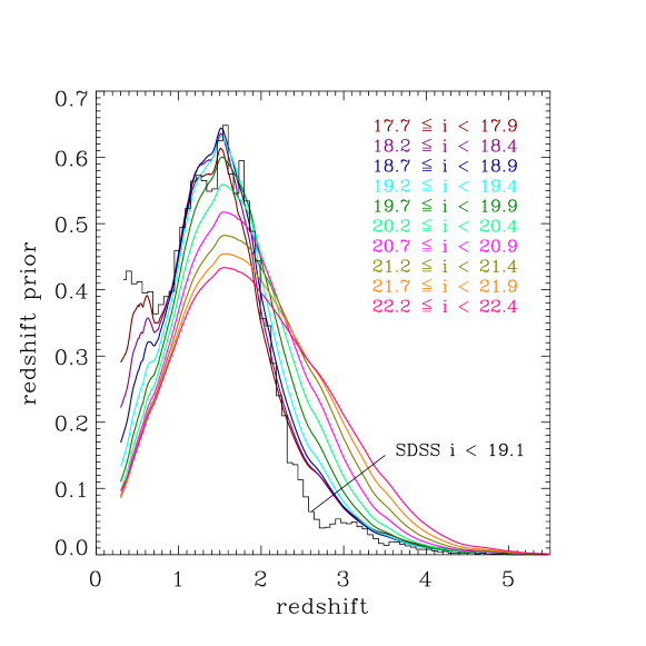
We use a sample of 103,601 spectroscopically-confirmed redshift $z\geq 0.3$ quasars from the SDSS DR7 quasar catalog (Richards et al., 2002; Schneider et al., 2010). We use all of these quasars to essentially model the color–redshift relation for quasars (but see below for the detailed description of our method). We combine the color–redshift relation with an apparent-magnitude dependent redshift prior obtained by integrating a model for the quasar luminosity function over the apparent-magnitude range of interest (Hopkins, Richards, & Hernquist, 2007). This prior for a few bins in apparent magnitude is shown in Figure 1; also shown is the difference between the Hopkins, Richards, & Hernquist (2007) redshift prior and the prior derived from the Richards et al. (2006) luminosity function. As the sample of quasars from the SDSS DR7 quasar catalog spans a wide range in luminosity that we apply to a narrow range in apparent magnitude and that we extrapolate to largely unexplored faint flux levels, we are ignoring correlations between quasar spectral properties and luminosity (e.g., Baldwin, 1977; Yip et al., 2004). These correlations mostly affect emission line shapes, such that they are washed out in broadband colors, especially compared to the intrinsic color-scatter.

3.2 UV data from the Galaxy Evolution Explorer

In addition to $ugriz$ optical data, we use UV data obtained by the Galaxy Evolution Explorer space mission (GALEX; Martin et al., 2005). GALEX has performed an all-sky imaging survey in two UV bands (FUV: 1350 to 1750 Å; NUV: 1750 to 2750 Å) down to $m_{\mathrm{AB}}\approx 20.5$ and a medium-deep imaging survey that reaches $m_{\mathrm{AB}}\approx 23$ (e.g., Bianchi et al., 2011). Some of the data used below to test the technique described in this article comes from the medium-deep survey, while much of the data used to train our technique comes from the shallower all-sky survey (because our training sample of quasars is drawn from the full $\approx 10,000$ deg² SDSS footprint), but this difference is largely offset by the fact that our training set is brighter than the faint part of the test set. GALEX GR5 observations were obtained between April 2003 and February 2009.

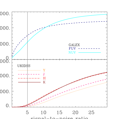
Rather than using GALEX catalog products (Morrissey et al., 2007) we use measurements of the UV fluxes obtained by force-photometering GALEX images (from GALEX Data Release 5) at the SDSS centroids (Aihara et al., 2011), such that we obtain low signal-to-noise PSF fluxes of objects not detected by GALEX. As we show below, these low signal-to-noise ratio observations are essential for better classification of redshift $z\geq 2$ quasars. We expect these measurements to be released as part of SDSS Data Release 9, scheduled for 2012. The top panel of Figure 2 shows the distribution of signal-to-noise ratio for SDSS quasars in the GALEX footprint. A total of 62,661 objects lie in the GALEX FUV footprint, 63,372 lie in the NUV footprint, and 62,628 are covered by both bandpasses.

3.3 NIR data from the UKIRT Infrared Deep Sky Survey

We also use NIR data to improve quasar classification and photometric redshift estimation. The UKIRT Infrared Deep Sky Survey (UKIDSS) is defined in Lawrence et al. (2007) and consists of five survey components with different wavebands, depths and footprints. For the study in this paper we use data from the UKIDSS Large Area Survey (LAS). Technical details about the UKIDSS LAS observing strategy are described in Dye et al. (2006).

The UKIDSS LAS aims to cover 4,000 deg² of the SDSS footprint in the Y, J, H and K wavebands. In this paper we use data from UKIDSS LAS DR7 which includes observations obtained between May 2005 and July 2009 inclusive. The UKIDSS LAS DR7 overlaps the SDSS imaging footprint over $\approx$ 2500 deg² and has median point source 5-sigma AB magnitude limits in Y, J, H and K of 20.9, 20.6, 20.2, and 20.2, respectively.

The UKIDSS data are acquired with the UKIRT Wide Field Camera (WFCAM; Casali et al. 2007). The UKIDSS photometric system is described in Hewett et al. (2006), and the calibration is described in Hodgkin et al. (2009). The pipeline processing and science archive are described in M. J. Irwin et al. (2012, in preparation) and Hambly et al. (2008).

As in the case of the GALEX data described in Section 3.2, we use force-photometered NIR fluxes at SDSS positions rather than UKIDSS catalog data. This “list-driven” information is derived from aperture photometry on Data Release 7 of the UKIDSS LAS. We choose an aperture radius of 1 arcsec. Of the 103,601 quasars in the SDSS DR7 quasar sample, 29,726 lie within the UKIDSS DR7 K-band footprint. Approximately 22,000 of these quasars are detected in the K band with also overlapping coverage in all four observed wavebands (Y, J, H and K) in the UKIDSS LAS DR7 source catalog. The bottom panel of Figure 2 shows the distribution of signal-to-noise ratio in the NIR for quasars in our training sample. Unlike for SDSS imaging, measurements in all four filters of the UKIDSS survey are not obtained during the same observing run—H and K observations are performed in the same observing block, while Y and J are conducted separately. Thus the sky coverage in different UKIDSS bands varies, and many objects are missing data in one or more of the four bands. The breakdown of training quasars with observations in the NIR by bandpass is: Y: 26,876; J: 27,328; H: 28,911; K:29,726. A total of 25,510 objects have measurements in all four bandpasses.

The differing epochs of the UKIDSS, GALEX, and SDSS can range up to 9 years in the observed frame. For a quasar with a redshift of 2 this is 3 years in the rest frame. The observed optical variability in radio quiet quasars over the rest frame 2 to 5 year timescale is observed to be in the range 0.1 - 0.2 mag and is a function of absolute magnitude (Hook et al., 1994). Vanden Berk et al. (2004) find that the variability amplitude decreases with rest-frame wavelength by a factor of two between 1500Å and 6000Å with an amplitude of $\approx$ 0.15 mag at 6000Å (see also Welsh et al. 2011).

Kozłowski et al. (2010b) have studied the mid-IR variability using multi-epoch Spitzer observations of a sample of $\approx$ 1000 active galactic nuclei and find that the rest-frame J band variability amplitude in the rest-frame timescale is $\approx$ 0.1 mag. In summary the quasars in this study are expected to vary by $\approx$ 0.3 and 0.1 magnitudes in the UV and NIR, respectively, over the elapsed period of the observations and this is less than the average photometric errors in the individual wavebands and significantly less than the range in colors.

Section 4 Flux–redshift density model

The photometric redshift technique XDQSOz is an adaptation of the XDQSO technique (Bovy et al., 2011) to include redshift explicitly in the model for the quasar population. XDQSOz achieves this by modeling the $p(\mathrm{flux},z|\mathrm{quasar})$ factor in equation (2), where the XDQSO technique modeled $p(\mathrm{flux}|\mathrm{quasar\ in}\ \Delta z)$ in three bins in redshift (corresponding to low-, medium-, and high-redshift quasars). As discussed in Section 2, this approach allows us to obtain full posterior distribution functions for the redshift of a photometrically classified quasar based on its broadband fluxes. Integrating this redshift probability distribution over a range of redshifts and properly normalizing this result using equation (7) gives a photometric quasar probability in the chosen redshift range that is, as we show below, competitive with the best available photometric quasar classification techniques, e.g., XDQSO.

To estimate the density of quasars in flux–redshift space we use extreme deconvolution (Bovy et al., 2009). As described in Section 3, our training set consists of the SDSS DR7 quasar sample, which consists mostly of bright, viz., dereddened $i<19.1$ mag ($i<20.2$ mag for $z>3$ sources), objects with small photometric uncertainties. The GALEX and UKIDSS data described in Sections 3.2 and 3.3 are much shallower than the SDSS data and many objects are not detected at high significance in these surveys, such that photometric uncertainties are not insignificant (see Figure 2). Additional complications are that these two supplemental surveys have not observed the full SDSS footprint and that the UKIDSS LAS footprint is different for the different NIR bands, such that we have heterogeneous missing data and heteroscedastic uncertainties. XD is uniquely suited to deal with these complications in the proper probabilistic manner. XD assumes that the flux uncertainties are known and that they are close to Gaussian, as is the case for PSF fluxes for point-sources in SDSS (Ivezić et al., 2003; Scranton et al., 2005b; Ivezić et al., 2007). We assume that the spectroscopic redshifts have vanishing uncertainties because their typical value of $\sigma_{z}\approx 0.004$ (Schneider et al., 2010) is orders of magnitude smaller than typical uncertainties in broadband photometric redshifts, which are set by the width of the quasar locus.

XD models the underlying, deconvolved distribution as a sum of $K$ $d$-dimensional Gaussian distributions, where $K$ is a free parameter that is set using an external objective (see Section 4.1). XD consists of a fast and robust algorithm to estimate the best-fit parameters of the Gaussian mixture.

4.1 Construction of the quasar flux–redshift model

The full quasar-density model is constructed by fitting the flux–redshift density of quasars in a number of bins in the $i$-band magnitude. As we use the same set of quasars in each bin with a different redshift prior—see the discussion in Section 3—we could instead have fit a single bin, e.g., the brightest. The other bins could have been constructed by dividing out the redshift prior of the first bin and multiplying in the redshift priors for the fainter bins. However, as we will show below, the advantage of a Gaussian representation of the flux–redshift density is that it allows integrals of this density over arbitrary redshift ranges to be calculated analytically. This leads to fast quasar-probability estimation. If we were instead to divide out the redshift prior and multiply in a different redshift prior, the resulting function would no longer be Gaussian and the numerical integration over redshift would be much more computationally expensive. Because our short-term objective is to run this algorithm on essentially all of the $\approx 10^{8}$ SDSS point sources and in the future on the $\approx 15$ PB of LSST catalog data (Abell et al., 2009), this computational advantage is important. After fitting the first bin, all other fits are initialized using the previous bin’s optimal solution; these extra fits all converge very quickly as the quasar flux–redshift density does not vary strongly with apparent magnitude. The redshift prior is shown for a few bins in apparent magnitude in Figure 1. If a different redshift prior is desired, one can divide out this prior and multiply in a new prior (these priors are included in the code release described in the Appendix). For example, if one would prefer to use the Richards et al. (2006) model for the quasar luminosity function, one would multiply the posterior distribution function for the redshift obtained using the fiducial Hopkins, Richards, & Hernquist (2007) prior with the factor shown in the bottom panel of Figure 1. This panel shows the ratio of the Richards et al. (2006) redshift prior to the Hopkins, Richards, & Hernquist (2007) prior in a number of apparent-magnitude bin. It is clear that there is only a significant difference at relatively large redshift and at faint magnitudes, where constraints on the luminosity function are sparse.

As for the XDQSO technique, we divide the quasar-density model into a factor describing, essentially, the color–redshift density of quasars—but we again use relative fluxes rather than colors—and another factor describing the apparent-magnitude distribution of quasars. We adopted this approach because the flux density of quasars has a dominant power-law shape corresponding to the number counts as a function of apparent magnitude, while the color distribution is much flatter. We write

$$p(\mathrm{fluxes},z|\mathrm{quasar})=p(\mathrm{fluxes\ relative\ to}\ i,z|\mathrm{quasar})\,p(i\mbox{-}\mathrm{band\ flux}|\mathrm{quasar})\,.$$ (8)

The apparent-magnitude factor does not depend on redshift. So, this factor is the same as used in the XDQSO method. The factor is calculated by the sum of the apparent-magnitude priors in Figure 1 of Bovy et al. (2011) weighted by the quasar densities in Table 1 of the same article. As quasar redshifts are always positive, we model the logarithm of the redshift. Since our training sample consists of point-like objects at redshift $z\geq 0.3$, about all at $z<5.5$, our model should only be trusted to return reasonable densities within this range.

In each bin we model the $d$-dimensional relative-flux–redshift density, where $d$ is the number of independent colors plus one (for redshift), of quasars using 60 Gaussians that are allowed to have arbitrary means, variance matrices, and amplitudes—the amplitudes are constrained to sum to one. We use the full set of 103,601, $z\geq 0.3$ quasars to train the final model, but in order to test whether we are under- or overfitting the data we performed a cross-validation test. To cross-validate we extract a random subset containing 10 percent of the full sample to use as an independent test data set. By training the model on the remaining 90 percent of the sample we can select the number of Gaussians that optimally predicts—i.e., predicts with the highest probability—the redshifts of objects in the test sample. The results from this procedure are shown in Figure 3. Our ability to better predict the test redshifts saturates around $K\approx 50$; we chose 60 Gaussians to represent the relative-flux density of quasars. Compared to the XDQSO method, which used 20 Gaussians each in three redshift bins, this revised approach uses the same number of Gaussians while representing an extra dimension (redshift). One might be concerned that because the Gaussians will preferentially be found in high-density, viz., low-redshift, regions, the density of medium- and high-redshift quasars is not adequately described in the XDQSOz model. We will see below that this is not the case and that XDQSOz performs similarly to XDQSO in selecting medium- and high-redshift quasars.

The full model consists of 47 bins of width 0.2 mag between $i=17.7$ and $i=22.5$, spaced 0.1 mag apart (adjacent bins overlap). As described above, the XD fits for all but the brightest bin are initialized using the best-fit parameters for the previous bin. Each bin uses the full set of 103,601 redshift $z\geq 0.3$ quasars.

In each of 47 bins we fit 60 $n$-dimensional Gaussians, yielding a total of $47\times(60\times[1+d+d(d+1)/2]-1)$ parameters. The $ugriz$-only model has 59,173 parameters, the model that also uses the two UV bands has 101,473 parameters, the model that adds the four NIR bands to the optical fluxes has 155,053 parameters, and the full UV-$ugriz$-NIR 11-dimensional model has 219,913 parameters. To obtain the total number of parameters for photometrically classifying quasars using XDQSOz, we need to add the number of parameters describing the stellar relative-flux density in 47 bins—from the XDQSO method—to this number, amounting to 14,053, 26,273, 42,253, and 61,993 parameters for the $ugriz$, $ugriz$+UV, $ugriz$+NIR, and $ugriz$+UV+NIR models, respectively. Models including UV or NIR data are trained using any available data, i.e., any object with a measured flux in any of the bandpasses is included in the training set.

4.2 Comparison of the model and observations

In this section, we assess the performance of the XD technique for modeling the relative-flux–redshift distribution of quasars, and provide examples which demonstrate that the XD technique produces excellent fits to the data. We demonstrate that the XD method does an excellent job of empirically calibrating the color–redshift relation; the ability of the XD technique to model the relative-flux density of quasars in the current XDQSOz context is excellent as well, but it is very similar to the performance in the XDQSO context and we refer the reader to Bovy et al. (2011) for a discussion of this performance.

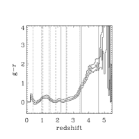
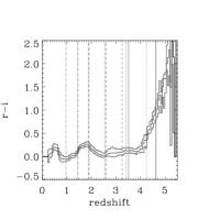
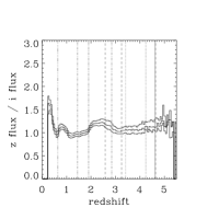
Figure 4 shows relative-flux–redshift and color–redshift diagrams of quasars for a single $i$-band magnitude bin. The conditional distribution of relative-flux as a function of redshift is shown here (although the model contains a full model of the density on this manifold); this emphasizes what is new in XDQSOz as compared to XDQSO. We see that the XD technique is superb at capturing the complexity of the quasar color locus, even at higher redshifts where the data are sparse and noisy. The locations where prominent emission lines cross the relevant SDSS filters are indicated, and it is clear that this drives much of the structure in the color–redshift relation.

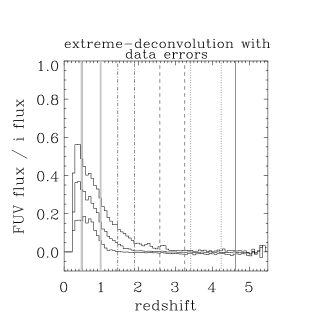
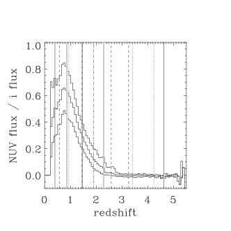
Figure 5 shows similar relative-flux–redshift diagrams for the UV fluxes in the model containing both optical and UV data. The agreement between the empirical model and the data is excellent. These diagrams clearly demonstrate that the UV flux of $z\gtrsim 1$ and $z\gtrsim 2.3$ quasars, for FUV and NUV respectively, is suppressed because of absorption below the Lyman limit ($\lambda 912$ Å) by intervening systems (Møller & Jakobsen, 1990; Picard & Jakobsen, 1993; Worseck & Prochaska, 2011). UV observations are an excellent tool to distinguish $z\approx 0.8$ quasars from $z\approx 2.3$ quasars, which have degenerate $ugriz$ colors and plague medium-redshift quasar selection (e.g., Ross et al., 2011), even at low UV signal-to-noise ratio.

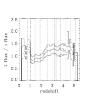
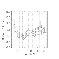
Figure 6 presents relative-flux–redshift diagrams for the four NIR fluxes in the XDQSOz model that contains optical and NIR data. The agreement between the XDQSOz model and the data is again excellent and the XDQSOz model captures all of the photometric redshift information contained in the NIR. We see that much of the variation in the color–redshift relation in the NIR is driven by the H$\alpha$ line (see also Glikman et al., 2006; Assef et al., 2010; Peth et al., 2011).

The model–data comparisons given in this section are only a small fraction of the model-assessment diagnostics that we performed. For example, we do not show the optical fits here in models that contain UV or NIR data, nor do we show the UV models and NIR models in the full $ugriz$-UV+NIR model, as all of these comparisons are very similar to the ones shown here.

Section 5 Targeting and photometric quasar classification with XDQSOz

We can use the XDQSOz model to photometrically classify and target quasars by calculating the probability that an object is a quasar based on its broadband fluxes. The probability that an object is a quasar in a redshift range $\Delta z$ is obtained by integrating the probability that an object is a redshift $z$ quasar over redshift. We start by using equation (5)

$$p(z,\mathrm{quasar}|\mathrm{fluxes}) \propto p(z,\{f_{j}/f_{i}\}|f_{i},\mathrm{quasar})\,p(f_{i},\mathrm{quasar})\,,$$ (9)

where $\{f_{j}/f_{i}\}$ is the set of fluxes relative to $f_{i}$ and $f_{i}$ is the $i$-band flux of the object. The normalization factor is given by

$$p(\mathrm{fluxes})=p(\mathrm{fluxes},\mathrm{star})+\int_{0}^{\infty}\mathrm{d}z\,p(z,\mathrm{fluxes},\mathrm{quasar})\,.$$ (10)

Because the apparent magnitude factor $p(f_{i},\mathrm{quasar})$ does not depend on redshift, the integral over redshift is only over the $p(z,\{f_{j}/f_{i}\}|f_{i},\mathrm{quasar})$ factor, which is modeled as a simple sum of Gaussian distributions.

For any given object we can simplify the mixture of $n$-dimensional Gaussian distributions to a mixture of one-dimensional Gaussian distributions for the redshift of the object. First, we find the bin in the $i$-band magnitude that best matches the object’s $i$-band magnitude and use the mixture-of-Gaussians representation of the relative-flux–redshift density in this bin. Assuming that the $n$-dimensional mixture of Gaussians has amplitudes $\alpha_{k}$, means $\mathbf{m}_{k}$, and variance matrices $\mathbf{V}_{k}$, we can condition each of the components on the measured relative flux $\mathbf{r}=\{f_{j}/f_{i}\}$ of the object and its uncertainty variance matrix $\mathbf{S}$ to find (e.g., Appendix B of Bovy et al. 2009)

$$m_{z,k} =m^{k}_{z}+\mathbf{V}^{k}_{zr}\,\mathbf{T}^{-1,k}_{rr}\,(\mathbf{r}-\mathbf{m}^{k}_{r})\,$$ (11)

$$\sigma^{2}_{z,k} =V^{k}_{zz}-\mathbf{V}^{k}_{zr}\,\mathbf{T}^{-1,k}_{rr}\,\mathbf{V}^{T,k}_{zr}\,$$ (12)

while the amplitudes of these one-dimensional Gaussian distributions are given by the posterior probability that the object was drawn from component $k$

$$\alpha_{z,k}=\frac{\alpha_{k}\,\mathcal{N}\left(\mathbf{r}|\mathbf{m}^{k}_{r},\mathbf{T}^{k}_{rr}\right)}{\sum_{l}\alpha_{l}\,\mathcal{N}\left(\mathbf{r}|\mathbf{m}^{l}_{r},\mathbf{T}^{l}_{rr}\right)}\,.$$ (13)

In these expressions $\mathbf{m}^{k}_{r}$ and $m^{k}_{z}$ are the relative flux and the redshift parts of $\mathbf{m}_{k}$, respectively; $\mathbf{T}^{k}_{rr}=\mathbf{V}^{k}_{rr}+\mathbf{S}$; $\mathbf{V}^{k}_{rr}$, $\mathbf{V}^{k}_{zr}$, and $V^{k}_{z}$ are the relative-flux–relative-flux, redshift–relative-flux, and redshift–redshift parts of $\mathbf{V}_{k}$, respectively; and $\mathcal{N}(\cdot|\cdot,\cdot)$ is the multivariate Gaussian distribution. $\mathbf{T}^{k}_{rr}$ includes the uncertainty variance matrix $\mathbf{S}$ because the necessary uncertainty convolution simply reduces to adding the observational uncertainty variance matrix to the intrinsic variance matrix for each Gaussian component.

Integrating this one-dimensional mixture of Gaussian distributions over an arbitrary redshift range results in a sum over error functions. Remembering that our model lives in $\log$ redshift space

$$\begin{split}\int_{z_{\mathrm{min}}}^{z_{\mathrm{max}}}\mathrm{d}z\,p(z,\{f_{j}/f_{i}\}|f_{i},\mathrm{quasar})&=p(\{f_{j}/f_{i}\}|f_{i},\mathrm{quasar})\\ &\quad\times\sum_{k}\frac{\alpha_{z,k}}{2}\left(\mathrm{erf}\left[\frac{\log z_{\mathrm{max}}-m_{z,k}}{\sqrt{2}\,\sigma_{z,k}}\right]-\mathrm{erf}\left[\frac{\log z_{\mathrm{min}}-m_{z,k}}{\sqrt{2}\,\sigma_{z,k}}\right]\right)\,,\end{split}$$ (14)

where the error function erf$[x]\equiv 2\int_{0}^{x}e^{-t^{2}}\mathrm{d}t\,/\sqrt{\pi}$. The first factor on the right-hand side of this equation is the integral over the entire redshift range $[0,\infty]$, which simplifies to

$$\begin{split}p(\{f_{j}/f_{i}\}|f_{i},\mathrm{quasar})&=\int_{0}^{\infty}\mathrm{d}z\,p(z,\{f_{j}/f_{i}\}|f_{i},\mathrm{quasar})\\ &=\sum_{k}\alpha_{k}\,\mathcal{N}\left(\mathbf{r}|\mathbf{m}^{k}_{r},\mathbf{T}^{k}_{rr}\right)\,\,\end{split}$$ (15)

i.e., the denominator in equation (13).

We can compare the quasar probabilities obtained by integrating the XDQSOz model over redshift to those from the XDQSO technique, which models the distribution of quasar fluxes in three wide redshift bins. Figure 7 shows the probabilities that 490,793 objects are medium-redshift ($2.2\leq z\leq 4.0$) quasars obtained by the two methods for objects in the SDSS imaging stripe 82. It is clear that most of the objects cluster tightly around the one-to-one line and that the two models are essentially the same for this redshift range.

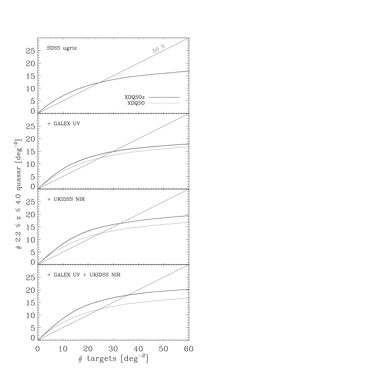
Figure 8 shows the efficiency of quasar targeting using both the XDQSO and the XDQSOz method for targeting medium-redshift ($2.2\leq z\leq 4.0$) quasars. This test uses a sample of medium-redshift quasars spectroscopically confirmed by BOSS —which also re-targets quasars previously identified in earlier surveys—in stripe 82. This quasar sample is expected to be highly complete, because it was targeted using the superior imaging in stripe 82 where there is variability information (Palanque-Delabrouille et al., 2011) and where a number of campaigns prior to BOSS have also obtained extensive spectroscopy. The sample has on average of 30 $z\geq 2.2$ quasars deg^-2 down to $g\approx 22$ mag, which is close to the number expected from current quasar luminosity functions (e.g., Hopkins, Richards, & Hernquist, 2007). We only use regions of stripe 82 that have more than 15 $z\geq 2.2$ quasars deg^-2. See Ross et al. (2011) and Bovy et al. (2011) for a more detailed description of the BOSS quasar target selection in general and this test set in particular.

The top panel of Figure 8 shows selection based on SDSS $ugriz$ fluxes alone. We see that the performance of the XDQSOz and the XDQSO techniques is essentially identical. The lower panels of this figure show how the selection improves when we add GALEX UV and UKIDSS LAS NIR observations, both of which are available for essentially all objects in SDSS stripe 82. The XDQSO models with UV and NIR data are models trained with these UV and NIR fluxes in the broad redshift ranges used by XDQSO. For all intended purposes the XDQSOz technique performs identically to the XDQSO technique for targeting medium-redshift quasars.

We have also checked the performance of the XDQSOz technique as compared to the kernel-density-estimation based photometric quasar classification technique of Richards et al. (2004, 2009a). We find results that are similar to those for the XDQSO technique as shown in Table 3 of Bovy et al. (2011): at low and medium redshift the XDQSOz technique performs slightly better than the XDQSO technique (and thus better than the KDE technique), while at high-redshift ($z>3.5$) XDQSOz performs slightly worse than XDQSO. This behavior is expected because the quasar training data do not include much data at high redshift. We thus do not probe the color–redshift relation at high redshift as well as the KDE approach, which included additional high-redshift data. Because we use the same stellar model as XDQSO, the same problem with sampling regions of low stellar density that we encountered for XDQSO persists for XDQSOz.

In summary, the XDQSOz technique performs almost identically to the XDQSO method for photometrically classifying objects as quasars—and thus for quasar targeting. XDQSOz has the advantage over XDQSO and any other photometric quasar classification scheme that it can classify quasars in arbitrary redshift ranges “on the fly” (i.e., without retraining the model).

We have computed XDQSOz quasar probabilities for all 160,904,060 point sources with dereddened $i$-band magnitude between 17.75 and 22.45 mag in the 14,555 deg² of imaging from SDSS Data Release 8 (Aihara et al., 2011) in three redshift ranges (0.3 $<z<2$, $2<z<3$, and $z>3$). Figure 9 shows the apparent $i$-band magnitude distribution of all of the objects with $17.8\leq i\leq 21.5$ mag in the expected BOSS spectroscopic footprint (Eisenstein et al., 2011) with XDQSOz probability larger than 0.5 over the specified redshift range. These apparent-magnitude distributions are smooth and well-behaved for low and medium redshifts. They also agree at the bright end with number counts derived from spectroscopic observations (Richards et al., 2006). At the faint end ($i\gtrsim 21$) the $i$-band number counts start to decline due to increasing photometric uncertainties and incompleteness of the SDSS imaging near the faint limit of SDSS.

The BOSS aims to detect the baryon acoustic feature (BAF) in the Ly$\alpha$ forest of background redshift $z\geq 2.2$ quasars. Not all quasars contribute equally to this measurement and, as shown by McDonald & Eisenstein (2007) and McQuinn & White (2011), both brighter quasars and quasars near redshift $z\approx 2.5$ are the most valuable. Combining Ly$\alpha$ BAF weights with the quasar probabilities as a function of redshift produced by XDQSOz, we can calculate the expected value of a quasar for the Ly$\alpha$ BAF measurement. Defining a value function $w(g,z)$, where $g$ is the dereddened $g$-band magnitude of the object, the expected value of an object is

$$\langle\mathrm{quasar\ value}\rangle=\int_{0}^{\infty}\mathrm{d}z\,w(g,z)\,p(z,\mathrm{quasar}|\mathrm{flux})\,.$$ (16)

By targeting objects with the highest expected value for a particular Ly$\alpha$ BAF survey—which is dependent on the exact observational characteristics of that survey—we could optimize the targeting of quasars for that BAF measurement.

The top panel of Figure 10 shows the number of medium-redshift quasars found by applying this value-based targeting for BOSS using the value function of McDonald & Eisenstein (2007). Value-based targeting finds about 1 quasar deg^-2 less than targeting based on the ranked medium-quasar probability list. The bottom panel shows that value-based targeting finds as much value as the straight probability-based targeting—but not more—such that the BAF measurement based on both samples should be equally precise. Straight probability-based targeting thus finds the same value while assembling a larger overall quasar sample. In addition, value-based targeting optimizes one experiment in a specific survey, whereas straight probability-based targeting returns information that is broadly applicable to a range of experiments and a range of surveys. Thus, in general, there is little to be gained from pursuing value-based targeting for BOSS.

To investigate whether the XDQSOz quasar selection technique is limited by contamination from galaxies that appear point-like at the faint flux levels to which we push quasar classification, we look at the fraction of objects that appear point-like in a single SDSS imaging-pass but are extended in co-added data on SDSS imaging stripe 82. We match the point sources in a typical SDSS imaging run to the co-added galaxy catalog on stripe 82 (Abazajian et al., 2009) and assess the fraction of point sources that are extended in the co-added data as a function of the $i$-band magnitude. This is shown in the top panel of Figure 11. We see that the fraction of point sources that are extended in the co-added imaging is only a few percent at relatively bright magnitudes, but almost reaches 50 percent at $i=22$ mag. To assess whether these point-like galaxies are a significant contaminant for the XDQSOz quasar selection, we calculate their quasar probabilities (over all redshifts). The fraction of point-like sources that are extended in the co-added imaging and that have quasar probabilities larger than 0.5 is shown as a function of the $i$-band magnitude in the lower panel of Figure 11. For comparison, the fraction of all point sources with quasar probability larger than 0.5 is shown as the dashed curve. Point-like galaxies make up only a small ($\lesssim 10$ percent) fraction of XDQSOz-selected photometric quasars. However, because galaxies unlike stars cluster similarly to quasars, even this small contamination fraction might significantly degrade precision quasar-clustering measurements without improved star–galaxy separation or proper modeling. Given the rising fraction of point-like galaxies with increasing magnitude in the top panel of Figure 11, point-like galaxies are likely to be the major contaminant for quasar selection at $i>23$ mag.

Section 6 Photometric redshifts with XDQSOz

We can use the XDQSOz flux–redshift density model to derive full posterior probability distributions for the redshift of photometric quasars taking the photometric uncertainties of the object fully into account. Because the main advantages of the XDQSOz technique for photometric redshift estimation are that it a) returns full PDFs and b) allows auxiliary data such as that furnished by UV and NIR surveys to be included, we focus on those points here. $ugriz$-only photometric quasar redshifts suffer from various degeneracies that are inherent to the $ugriz$ filter system. While including appropriate apparent-magnitude dependent redshift priors—as we do here—can partially relieve these degeneracies somewhat, no photometric redshift technique can entirely remove these degeneracies and XDQSOz is no exception (as we will see below). Crucially, even low signal-to-noise ratio UV and NIR data can cleanly resolve these degeneracies.

For each object the posterior probability distribution for its redshift, based on its measured broadband fluxes, is calculated by finding the apparent-magnitude bin that best matches the object’s dereddened $i$-band magnitude. The posterior probability distribution is given by the mixture of 60 one-dimensional Gaussian distributions, with means, variances, and amplitudes given in equation (11), (12), and (13), respectively. This posterior probability distribution can be calculated based on $ugriz$ fluxes, or with additional UV or NIR information if available.

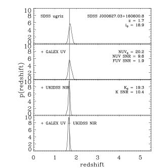
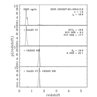
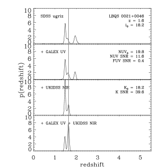
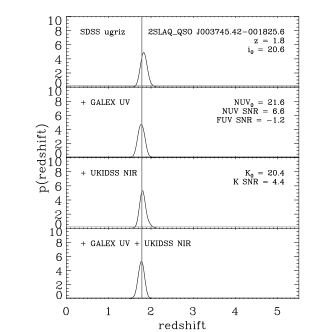
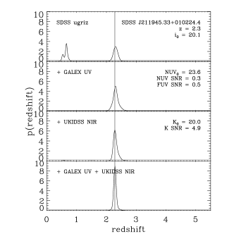
We show four examples of such redshift PDFs in Figure 12 for objects from the SDSS DR7 quasar catalog that have measurements in all of the UV and NIR filters. These objects are from the sample used to train the flux–redshift quasar model, but, as we discuss in more detail below, we nevertheless believe that they provide an adequate representation of the performance of the XDQSOz technique. These objects are chosen to demonstrate the power and weaknesses of the $ugriz$, UV, and NIR data for photometric redshift estimation, and are therefore not a random subset of the data. We discuss the overall performance below.

The top left panel shows an example where the $ugriz$ fluxes suffice to accurately and precisely measure the redshift, and how the (relatively high signal-to-noise ratio) UV and NIR measurements tighten the PDF significantly. The top right panel shows an example where the extremely low UV flux basically vetoes the low-redshift peak that is present in the $ugriz$-only redshift PDF. If one were to use a simple non-detection GALEX catalog at 5$\sigma$ this result would not have been clear, because this object could have had the mean $z\approx 0.8$ UV flux and still not be detected by GALEX. The ability of the XDQSOz technique to use and interpret low signal-to-noise ratio data is therefore crucial in this example.

A weakness of the auxiliary UV data is apparent in the lower left panel. Here we see a $z=1.6$ quasar that is much brighter than the average quasar at this redshift in the UV, such that the addition of the UV data mistakenly chooses the low-redshift peak of the degenerate $ugriz$ redshift PDF. However, the NIR data are able to overcome this error and the addition of all the data confidently assigns this object a close-to-correct redshift. The lower right panel of Figure 12 shows another amusing example.

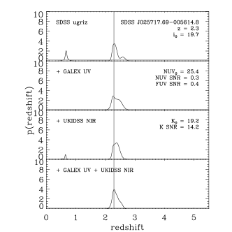
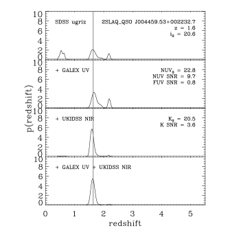
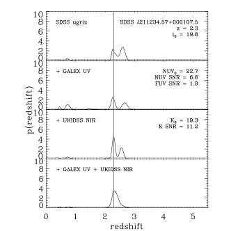
In addition to testing the XDQSOz technique using the SDSS DR7 quasar sample, we have also drawn a sample of quasars located in the SDSS imaging in stripe 82 discovered as part of the 2SLAQ survey (Croom et al., 2009) and BOSS (Ross et al., 2011; Palanque-Delabrouille et al., 2011). These quasars are generally fainter than the SDSS quasars and therefore they represent a stringent, independent test of the XDQSOz technique’s ability to return accurate redshift PDFs at faint magnitudes. We have specifically selected all $0.3\leq z\leq 5.5$ quasars with dereddened $i\geq 19.1$ mag from the 2SLAQ sample and all quasars on the SDSS imaging stripe 82 newly discovered by BOSS and use their single-pass SDSS photometry. Because most of these objects lie in the SDSS equatorial stripe, many of them have measurements from GALEX and UKIDSS LAS.

Figure 13 shows posterior probability distributions for the redshift of two objects from the 2SLAQ catalog and two from the BOSS sample. The trends that were apparent for the SDSS DR7 quasars in Figure 12 are also evident for these fainter objects. The UV and NIR fluxes for these objects have, in general, been measured much less precisely than those discussed above, but the auxiliary data still provide valuable extra information about the redshift.

While most of the examples in Figures 12 and 13 have a considerable posterior probability mass associated with the correct redshift, even when multiple peaks are present in the redshift PDF, this situation is generic—in that inspections of many redshift PDFs show that it is rare to have no posterior probability mass associated with the spectroscopic redshift.

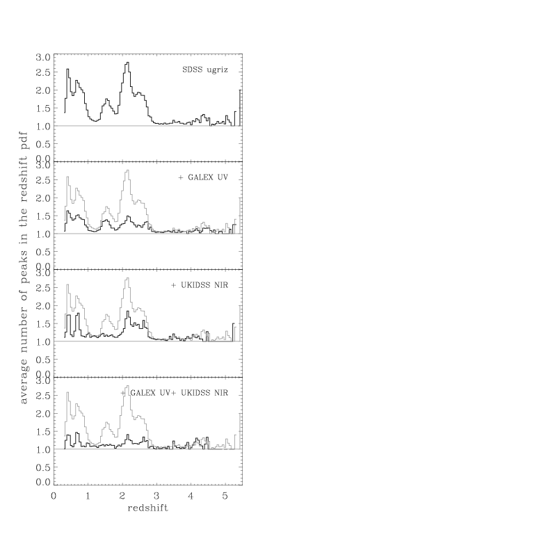
As a simple statistic for the degeneracy in the redshift PDF we examine the number of distinct peaks as a function of redshift. A single peak in the PDF is defined here as the widest contiguous region where the PDF is above the uniform distribution between redshift 0.3 and 5.5 (i.e., flat in redshift). The top panel of Figure 14 shows the average number of such peaks as a function of redshift. This statistic clearly shows the main degeneracies of $ugriz$-based photometric quasar redshifts. Basically the entire $z<1$ region, a region around $z=1.5$, and the $2.0\leq z\leq 2.7$ redshift range are degenerate. Higher redshift quasars are readily identified as such using the $ugriz$ colors (e.g., Fan et al., 1999). From the lower panels we see that the addition of UV and NIR data softens all of these degeneracies. Essentially no degeneracies remain using the combination of all the UV, optical, and NIR data (lower panel of Figure 14). Additionally, requiring that distinct peaks in the photometric-redshift PDF need to have a minimum integrated probability (e.g., defining a peak as a contiguous region above the uniform distribution with $>0.05$ integrated redshift probability) gives similar results for the number of peaks and the improvement when adding UV and NIR data.

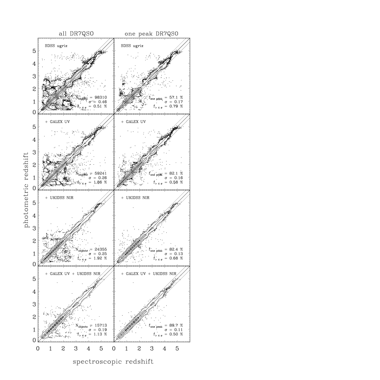
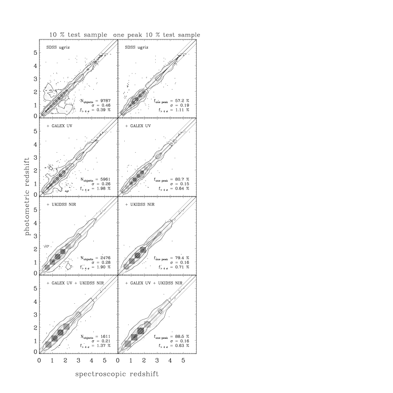
Figure 15 shows the traditional spectroscopic-redshift vs. photometric-redshift diagram for quasars in the SDSS DR7 quasar sample, for various combinations of wavelength regimes. The right panels restrict the sample to those objects for which the redshift PDF has only a single peak and as such can be accurately described by a single photometric redshift (plus uncertainty). In the top left panel all of the $ugriz$-related degeneracies are clearly present and the right panel shows that by restricting the sample to single-peaked PDFs most of these degeneracies vanish, albeit at the cost of entire redshift ranges—most notably redshift-range $2.0\lesssim z\lesssim 2.5$ quasars. The addition of UV and especially that of NIR observations a) greatly reduces the degeneracies as witnessed by the diminishing structure in the spectroscopic vs. photometric redshift plane and the increasing fraction of objects with a single peaked redshift PDF, and b) significantly reduces the scatter. In the individual panels we report the number of 4$\sigma$ outliers rather than the number of $|\Delta z|>0.3$ objects; the latter number is somewhat meaningless without comparing it to the scatter, but to guide the eye we have included the $|\Delta z|=0.3$ lines. The scatter is calculated without outlier-rejection. We note that—here and in the test below—the distribution of the $i$-band magnitude is unchanged when restricting the sample to objects with measured GALEX or UKIDSS fluxes; restricting to objects with NIR fluxes actually creates a fainter sample, because many faint quasars in the SDSS imaging stripe 82 have been observed by UKIDSS LAS, while many brighter quasars are located outside of the UKIDSS LAS footprint.

With the addition of UV and NIR data most objects have accurate and precise single-peaked photometric redshifts over the entire $0.3\leq z\leq 5.5$ redshift range: 97 percent of all objects with UV and NIR data and 99 percent of the subset with single-peaked redshift PDFS have photometric redshifts within $|\Delta z|<0.3$; for $|\Delta z|<0.1$ these numbers are 84 percent and 86 percent respectively. This is a significant improvement over $ugriz$-only photometric redshifts, where we find 86 percent of objects within $|\Delta z|<0.3$. Similarly, Weinstein et al. (2004) found 83 percent of objects in this range.

Photometric and spectroscopic redshifts in Figure 15 are compared for objects in the sample used to train the XDQSOz technique. As such, one might object that this is not a fair representation of the performance of the XDQSOz technique. But, the relationship between the photometrically estimated redshift PDF and the spectroscopic redshift of a training object for XDQSOz is through the many-parameter flux–redshift density model. This model includes reweighting objects in the training set according to a redshift prior. There is therefore no direct connection between output photometric redshifts and input spectroscopic redshifts— as there is, for example, in nearest-neighbor approaches to photometric redshift estimation (Ball et al. 2007, 2008). The fact that Figure 15 contains all of the expected redshift degeneracies for $ugriz$-based photometric redshifts is further proof of this independence: if there were a dependent connection we would not suffer from these degeneracies.

To further test this issue we have divided our sample into a 90 percent training sample and a 10 percent test sample, as described above in Section 4.1. We redo the spectroscopic-redshift vs. photometric-redshift comparison for the 10 percent sample using the model trained in the 90 percent of remaining data—the results are in Figure 16. Because the 10 percent sample is much smaller than the full SDSS DR7 quasar sample the statistics are noisier, but the trends are the same as in Figure 15.

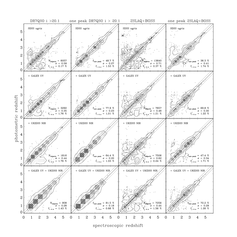
To test the XDQSOz technique at fainter magnitudes, in Figure 17 we compare spectroscopic redshifts to photometric redshifts for $i>20.1$ objects in the SDSS DR7 quasar catalog and for objects in the combined 2SLAQ and BOSS sample. The trends in this figure are the same as those for the brighter SDSS quasar sample and the scatter is somewhat larger; however, the photometric redshifts remain clustered around the spectroscopic redshifts with no discernible bias. Even for the faint 2SLAQ and BOSS sample, the addition of low signal-to-noise ratio UV and NIR data leads to a significant increase in accuracy and precision.

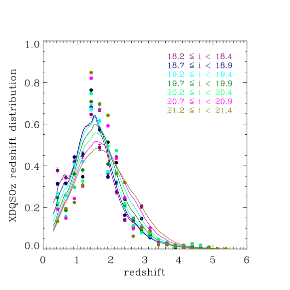
Using the technique described in this section we have computed photometric redshifts for all point sources in the expected BOSS spectroscopic footprint with XDQSOz quasar probabilities larger than 0.5 and $17.8\leq i\leq 21.5$ mag. The distribution of peaks of the photometric-redshift distribution for these objects is shown in Figure 18 in a few apparent-magnitude bins (those bins from Figure 1 that lie within the $17.8\leq i\leq 21.5$ apparent-magnitude range. The overall shape of the redshift distribution in each $i$-band bin is similar to the redshift prior calculated from the Hopkins, Richards, & Hernquist (2007) luminosity-function model. However, the redshift-dependent efficiency of photometric quasar classification and redshift estimation is apparent in this comparison and the low classification efficiency at $2.5\lesssim z\lesssim 3.5$ depresses the distribution in that range while increasing the significance of the $z\approx 1.5$ peak.

All of the results in this section have assumed the Hopkins, Richards, & Hernquist (2007) redshift prior, shown in Figure 1. Using the difference between the Hopkins, Richards, & Hernquist (2007) and Richards et al. (2006) redshift prior, given in the bottom panel of Figure 1, we can assess the difference in photometric redshift distribution when using these two alternatives to the quasar luminosity function. The bottom panel of Figure 1 shows that the only significant difference between these two models is at relatively high redshift ($z\gtrsim 2.5$) and near the SDSS detection limit ($i\gtrsim 21$ mag). Strongly single-peaked photometric redshift distribution functions, such as many of those shown in Figures 12 and 13, are not affected by even order-of-magnitude changes in the redshift prior, especially when UV or NIR data are available. It is clear from Figures 15 and 17 that, on average, the influence of a different redshift prior will be limited, as the main differences lie at higher redshift, where the SDSS colors provide relatively unambiguous photometric redshifts (as shown by the lack of degeneracies at higher redshift in the photometric versus spectroscopic redshift plane). As the photometric redshift distributions are only marginally affected by the use of a different prior, classification based on integration over these redshift PDFs also does not depend strongly on the details of the redshift prior.

Section 7 Discussion

7.1 Comparison with other methods

We have previously discussed other photometric redshift estimation techniques for quasars in Section 2. Comparing Figure 15 to similar diagrams in Budavári et al. (2001); Richards et al. (2001b); Ball et al. (2007, 2008) we see, at least qualitatively, that the XDQSOz technique performs similarly when applied to the $ugriz$ fluxes of bright, high signal-to-noise ratio objects. We did not expect to perform better as the near-degeneracies in the $ugriz$ color–redshift plane are real and the quasar locus is broad. The advantage of the XDQSOz technique over these other techniques is that it can be applied to faint objects and that it can incorporate UV and NIR observations, even at low signal-to-noise ratio, to improve photometric redshift estimation and quasar classification.

No other method exists to calculate photometric quasar probabilities over arbitrary redshift ranges. By comparing with state-of-the-art photometric quasar classification using kernel-density estimation or Gaussian mixture density deconvolution (Richards et al., 2004; Bovy et al., 2011), we have shown that the photometric quasar probabilities obtained by integrating the photometric redshift PDF over redshift are as good as those trained on the redshift range in question.

7.2 Including additional information

Two additional sources of information relevant to photometric quasar classification and redshift estimation stand out as the next steps toward a full quasar model, although neither of these is currently available over the large areas of the sky surveyed by projects such as the SDSS: photometric variability and differential-chromatic-refraction-induced astrometric offsets for quasars. Of these, photometric variability is the easiest to include in the quasar classification technique discussed here, as we can ignore the redshift information contained in the variability, because this information seems to be limited (MacLeod et al., 2011a). As such, a photometric variability likelihood for quasars and stars could be multiplied with the flux–redshift likelihood employed and modeled here to perform simultaneous color and variability selection. The combination of photometric variability and color information will lead to accurate photometric quasar classification and redshift estimation in the LSST era.

The strong spectral features of quasars induce positional offsets to standard differential-chromatic-refraction corrections (Kaczmarczik et al., 2009). These positional offsets are redshift dependent much as quasar colors are redshift dependent because of spectral features moving through individual filters (see, e.g., Figure 4). Thus, these offsets could be used to break redshift degeneracies. Accomplishing this in the XDQSOz flux–redshift density context necessitates adding the astrometric offsets into the density model. Because the astrometric offsets are zenith angle dependent, these models would have to be constructed for a range of airmasses, or airmass could be added as an additional dimension. As astrometric redshifts are a subtle and difficult-to-measure effect, the deconvolution aspect of the XD density-estimation technique could be useful.

7.3 Generalized photometric object classification and characterization

The technique described in this article is a step toward a generalized method for object classification and characterization from broadband photometric data, which will become increasingly relevant in this era of major wide-field imaging surveys. While our quasar model includes redshift in addition to the broadband fluxes of an object, our star model does not because stars do not possess a cosmological redshift. Stars are characterized by other properties—e.g., distance and metallicity—that are often estimated photometrically (e.g., Jurić et al., 2008; Ivezić et al., 2008). As we are interested here in quasar classification and characterization, our model implicitly marginalized over stellar properties. However, as part of a general object classification pipeline, these properties should be included—and the technique developed in this paper could be applied.

More importantly, the general framework outlined in Section 2 and the specific implementation in Sections 4 and 5 show that we can perform classification when different models are characterized by different parameters—even different numbers of parameters. This aspect is especially relevant in the context of quasar selection based on variability. Quasar variability is commonly modeled as a stochastic Gaussian Process (Kelly et al., 2009; Kozłowski et al., 2010a) characterized by a small number of parameters. Recently it has been shown that this framework allows for a clean selection of quasars because most stars—the main contaminants for quasar targeting currently—in general do not vary over long time baselines. In this type of selection, however, quasars and stars are often modeled (or fit) using the same stochastic model, which is inappropriate for the stars (Schmidt et al. 2010; MacLeod et al. 2011b; however, see Butler & Bloom 2010).

The use of a stochastic model for variability-based star–quasar separation is particularly problematic for RR Lyrae stars—a common contaminant in color-based classification of quasars in some redshift ranges. RR Lyraes are known to vary periodically rather than stochastically. In the framework we use in this article all classes of objects can be described using models appropriate for the class—e.g., stochastically varying objects with a cosmological redshift for the quasars and non-variable sources for most stars—because object classification only uses marginalized probabilities, that is, probabilities marginalized over the internal properties of each class (cf. equation [5]). Describing each class with a model appropriate for that class should lead to better classification and simultaneous object classification of sources into all classes.

As photometric quasar classification moves to ever fainter flux levels, contamination from point-like galaxies becomes increasingly important. As discussed by Bovy et al. (2011), unresolved galaxies are implicitly taken into account in our model because our training set of “stars” is actually a set of non-variable point-like objects that therefore includes faint galaxies. This model of galaxies again implicitly marginalizes over galaxy properties, most notably the redshift of the galaxy. Photometric redshift estimation for galaxies is closely related to obtaining photometric redshifts for quasars, but the galaxy photometric redshift techniques tend to rely more on templates in their model building, while quasars are modeled in a more empirical manner (e.g., Benítez, 2000). However, this distinction is not fundamental and the general framework discussed here still applies. Template-based models are just another way of obtaining the probability $p(\mathrm{fluxes}|\mathrm{galaxy})$ or $p(\mathrm{fluxes},z|\mathrm{galaxy})$.

7.4 Quasar tracks

The XDQSOz model of Section 4 also contains the distribution of broadband fluxes as a function of redshift $p(\mathrm{fluxes}|z,\mathrm{quasar})$ such as is used to compute mean quasar color tracks. This probability density is obtained from the full XDQSOz model flux–redshift density by conditioning on redshift. For the relative flux this leads to a mixture of Gaussians with means, variances, and amplitudes given by expressions similar to those in equations (11) and (13)—essentially, relative flux and redshift need to be interchanged in those equations. Properties of this distribution can be calculated from the mixture of Gaussians. For example, the mean quasar relative flux (or color) as a function of redshift is obtained by weighting the means of the Gaussian components using the redshift-dependent amplitudes. Code to calculate the mean quasar color track is included in the package described in the Appendix.

Section 8 Conclusion

In this article we have introduced a new approach to photometric quasar classification that can simultaneously classify quasars and characterize their redshifts based on broadband photometry. This technique, XDQSOz, is an extension of the XDQSO technique of Bovy et al. (2011) that adds the unknown redshift as an extra parameter to the quasar model to obtain the likelihood $p(z,\mathrm{fluxes}|\mathrm{quasar})$ that is central to both quasar classification and photometric redshift estimation. We have shown that this combined approach is both the best current quasar classification technique—it has similar performance as the XDQSO method—and a competitive photometric redshift method. Compared to other approaches to photometric redshift estimation for quasars it has the advantage that it can incorporate additional UV and NIR data, even at low signal-to-noise ratio, and can be extended to fainter flux levels where photometric uncertainties are significant. Using samples of quasars drawn from the SDSS, 2SLAQ, and BOSS spectroscopic catalogs we have demonstrated this increased performance down to $g\approx 22$ mag. The addition of UV and NIR data to the photometric redshift estimation problem essentially breaks all of the redshift degeneracies inherent to the $ugriz$ filter set.

Code to use the XDQSOz technique for classification and redshift estimation, including the ability to calculate full posterior probability distributions for the redshift, are made publicly available. This code is briefly described in the Appendix.

Appendix A Code

The XDQSOz code for target selection, classification, and photometric redshift estimation is publicly available at

http://www.sdss3.org/svn/repo/xdqso/tags/ .

The code can be downloaded by svn export of the most recent tag. The documentation of the most recent version of the code can be found at

http://www.sdss3.org/svn/repo/xdqso/tags/v0_6/doc/build/html/index.html .

Future updates will have documentation available at a similar URL.

The XDQSO/XDQSOz package contains routines for quasar classification using the XDQSO and XDQSOz techniques. It also contains code to calculate posterior probability distributions for the quasar redshift of objects based on input psfflux and psfflux_ivar; these can be found in standard SDSS data files such as the ‘sweeps’ files

The XDQSOz models for the quasar color–redshift density are contained in the data/ directory. They are in the form of FITS files containing the XD models for all of the bins in apparent magnitude, with one file for each combination of SDSS with GALEX and UKIDSS. Each FITS file contains 47 extensions, where extension $k$ contains a structure with the amplitudes (tag xamp), means (tag xmean), and covariance matrices (tag xcovar) for bin $k$ in $i$-band magnitude. The zeroth dimension of the Gaussian represents the natural logarithm of the redshift, followed by SDSS, GALEX, and UKIDSS fluxes (where relevant) in this order, and ordered as NUV/FUV for the GALEX, and YJHK for the UKIDSS.

Figure 1: Prior distribution for the redshift in a few $i$-band bins (top panel). The histogram shows the redshift distribution of 69,994 quasars from the SDSS DR7 quasar catalog with dereddened $i$-band magnitude $<19.1$, where the quasar catalog is highly complete (except for the redshift range 2.5 $\leq z\leq 3.2$). The bottom panel shows the difference in prior when using the Richards et al. (2006; hereafter R06) quasar luminosity function rather than the fiducial Hopkins, Richards, & Hernquist (2007; hereafter HRH07) model.

Figure 2: Cumulative distribution of signal-to-noise ratio for those quasars in the SDSS DR7 quasar sample observed by GALEX ($\approx$ 62,628 objects; top panel) and UKIDSS LAS ($\approx$ 25,510 objects; bottom panel). See Sections 3.2 and 3.3 for the number of objects in each individual bandpass. The five-sigma detection limit is indicated.

Figure 3: Total probability of the spectroscopic redshifts of objects in the 10 percent test sample given their $ugriz$ fluxes using models with different numbers of Gaussians trained on the remaining 90 percent of objects in the SDSS DR7 quasar catalog.

Figure 4: Flux–redshift and color–redshift diagrams for the 18.6 $\leq i<18.8$ bin in apparent magnitude for the 103,577 objects in the quasar catalog. The first column shows a conditional plot of a sampling from the extreme deconvolution fit with the errors from the quasar data added; the second column presents the quasar data resampled according to the quasar luminosity function as described in Section 3 and in more detail in Bovy et al. (2011). All fluxes are relative to the $i$-band flux of the object. The third and fourth columns show the same information as the first and second columns, but for colors. Linear conditional densities are shown as well as the 25, 50, and 75 quantile-lines. The vertical lines denote where prominent emission lines pass in and out of the relevant filters (Ly$\alpha$: full; CIV: dotted; CIII: dashed; MgII: dash-dotted; H$\alpha$: dash-dot-dot-dotted). Although only the conditional relation between redshift and flux/color is shown here, we fit the full density in the flux–redshift space.

Figure 5: Flux–redshift diagrams for the $18.6\leq i<18.8$ bin in apparent magnitude for the 62,628 SDSS quasars with GALEX observations in both GALEX bandpasses. The left column shows a conditional plot of a sampling from the extreme deconvolution fit with the errors from the quasar data added; the right column displays the quasar data resampled according to the quasar luminosity function as described in Section 3. All fluxes are relative to the $i$-band flux of the object. Densities, curves, and vertical lines are as in Figure 4. The thick light-gray bands show where the Lyman limit ($\lambda 912$ Å) crosses the UV filters.

Figure 6: Same as Figure 5, but for the 25,510 SDSS quasars that have UKIDSS LAS observations in all four UKIDSS bandpasses.

Figure 7: Comparison between mid-redshift ($2.2\leq z\leq 4.0$) quasar probabilities computed using XDQSO, that is, based on flux-density models in broad redshift ranges, and XDQSOz, i.e., obtained by integrating flux–redshift–density models over the relevant redshift range, for 490,793 objects in SDSS stripe 82 based on single-imaging-run flux measurements. Conditional 25, 50, and 75 percent quantiles are shown.

Figure 8: Mid-redshift ($2.2\leq z\leq 4.0$) quasar selection efficiency for XDQSO and XDQSOz as a function of target density for objects in SDSS Stripe 82 based on single-imaging-run flux measurements. The top panel bases selection solely on SDSS $ugriz$ fluxes, the lower panels add GALEX NUV and FUV medium-deep measurements as well as UKIDSS YJHK photometry, both of which are available for almost all Stripe-82 sources, through force-photometering GALEX and UKIDSS LAS imaging data at SDSS positions. The 50 percent selection efficiency is indicated and the $ugriz$-only curve for XDQSOz is repeated in gray in each panel.

Figure 9: Apparent $i$-band magnitude distribution of all point sources in the expected SDSS-III BOSS footprint with XDQSOz quasar probability larger than 0.5 over the indicated redshift range and dereddened $i$ between 17.8 mag and 21.5 mag. Diamonds indicate number counts from the SDSS spectroscopic survey (Richards et al., 2006).

Figure 10: Comparison between “value-based” and straight probability-based quasar selection for BOSS. “Value-based” selection ranks targets on the expected signal-to-noise ratio of the Lyman-$\alpha$ forest, while probability-based selection ranks on $P(2.2\leq z\leq 4.0$ quasar). The top panel shows the number of mid-redshift quasars found by each method as a function of the target density; the bottom panel shows the value of the selected quasars. Note that some $z<2.2$ quasars are valuable for the Lyman-$\alpha$ forest BAF measurement.

Figure 11: Point-like galaxy contamination of color-based quasar selection: The top panel shows the fraction of point sources in a single imaging-pass of SDSS stripe 82 that are extended in the co-added stripe-82 imaging (Abazajian et al., 2009) as a function of the $i$-band magnitude. The bottom panel shows the fraction of such point-like galaxies that have an XDQSOz quasar probability (over all redshifts) larger than 0.5. The dashed curve in the bottom panel shows the fraction of all point-sources that have an XDQSOz quasar probability larger than 0.5. Even though point-like galaxies start to dominate the number counts around $i$ = 22 mag, they only make up a small fraction of photometrically selected quasars at all magnitudes.

Figure 12: Posterior distribution functions for the photometric redshift of four quasars from the SDSS DR7 quasar catalog. The top panel in each plot shows the redshift posterior distribution function based only on $ugriz$ fluxes; the lower panels add UV (NUV and FUV) and NIR measurements (in YJHK). The vertical line shows the spectroscopic redshift. The horizontal line represents the uniform distribution over $0.3\leq z\leq 5.5$.

Figure 13: Same as Figure 12 but for objects from the fainter test sample, composed of quasars from the 2SLAQ survey and from the BOSS in SDSS stripe 82.

Figure 14: Average number of peaks in the posterior distribution function for the photometric redshift as a function of spectroscopic redshift for the SDSS DR7 quasar sample. A peak is defined as a contiguous region where the posterior distribution exceeds the uniform distribution on 0.3 $\leq z\leq 5.5$. The top panel uses photometric redshift predictions from only $ugriz$ data; the lower panels add UV and NIR data. The optical-only curve is repeated in the lower panels in gray.

Figure 15: Spectroscopic versus photometric redshift for quasars from the SDSS DR7 quasar catalog. Photometric redshifts are maximum a posteriori redshifts, i.e., they are at the peak of the photometric redshift posterior distribution function. The left column shows all sources; the right column shows sources that have only a single peak in their photometric redshift posterior distribution, that is, they have only one contiguous region in their posterior distribution where the distribution exceeds the uniform distribution on 0.3 $\leq z\leq$ 5.5. The top row shows predictions based only on $ugriz$ fluxes, the lower panels add UV and NIR information, restricted to those objects that were observed in both NUV and FUV for GALEX, and in all four YJHK UKIDSS filters. The one-to-one line is shown in black and the $|\Delta z|=0.3$ lines are shown in gray.

Figure 16: Same as Figure 15, but for a random sample of 10 percent of objects from the SDSS DR7 quasar catalog, with the model trained on the remaining 90 percent of quasars.

Figure 17: Spectroscopic versus photometric redshifts for the $i>20.1$ subset of the SDSS DR7 quasar catalog as well as for the faint test sample composed of quasars from the 2SLAQ survey and the BOSS. The two columns on the left are as for Figure 15, but restricted to those objects with $i>20.1$ mag. The two columns on the right are as for the leftmost columns, but for the 2SLAQ + BOSS test sample.

Figure 18: Distribution of the peak of the photometric redshift distribution for all objects in the expected SDSS-III BOSS survey in a few apparent-magnitude ranges. The curves are the redshift priors calculated from the Hopkins, Richards, & Hernquist (2007) luminosity-function model. The color coding is the same as in Figure 1. The overall shape of the redshift distribution is similar to the prior distribution, except for the drop in $2.5\leq z\leq 3.5$ due to the decreased efficiency of photometric quasar classification based on SDSS photometry.

References

- Abazajian et al. (2009) Abazajian, K. N., et al., 2009, ApJS, 182, 543
- Abell et al. (2009) Abell, P. A., et al., 2009, The LSST Science Book, arXiv:0912.0201v1 [astro-ph]
- Aihara et al. (2011) Aihara, H., et al., 2011, ApJS, 193, 29
- Assef et al. (2010) Assef, R. J., et al., 2010, ApJ, 713, 970
- Atlee & Gould (2007) Atlee, D. W. & Gould, A., 2007, ApJ, 664, 53
- Baldwin (1977) Baldwin, J. A., 1977, ApJ, 214, 679
- Ball et al. (2007) Ball, N. M., Brunner, R. J., Myers, A. D., Strand, N. E., Alberts, S. L., Tcheng, D., & Llorà, X., 2007, ApJ, 663, 774
- Ball et al. (2008) Ball, N. M., Brunner, R. J., Myers, A. D., Strand, N. E., Alberts, S. L., & Tcheng, D., 2008, ApJ, 683, 12
- Baum (1962) Baum, W. A., 1962, in Problems of Extra-Galactic Research, Proceedings from IAU Symposium no. 15, edited by McVittie, G. C., 390
- Benítez (2000) Benítez, N., 2000, ApJ, 536, 571
- Bianchi et al. (2011) Bianchi, L., Efremova, B., Herald, J., Girardi, L., Zabot, A., Marigo, P., & Martin, C., 2011, MNRAS, 411, 2770
- Bovy et al. (2009) Bovy, J., Hogg, D. W., & Roweis, S. T. 2009, Ann. Appl. Stat. 5, 2B, 1657, arXiv:0905.2979
- Bovy et al. (2011) Bovy, J., et al., 2011, ApJ, 729, 141
- Bowen et al. (2006) Bowen, D. V., et al., 2006, ApJ, 645, L105
- Budavári et al. (2001) Budavári, T., et al., 2001, AJ, 122, 1163
- Butler & Bloom (2010) Butler, N. R. & Bloom, J. S., 2010, AJ, 141, 93
- Casali et al. (2007) Casali, M., et al., 2007, A&A, 467, 777
- Chiu et al. (2007) Chiu, K., Richards, G. T., Hewett, P. C., & Maddox, N., 2007, MNRAS, 375, 1180
- Connolly et al. (1995) Connolly, A. J., Csabai, I., Szalay, A. S., Koo, D. C., Kron, R. G., & Munn, J. A., 1995, AJ, 110, 2655
- Croom et al. (2001) Croom, S. M., Warren, S. J., & Glazebrook, K., 2001, MNRAS, 328, 150
- Croom et al. (2009) Croom, S. M., et al., 2009, MNRAS, 392, 19
- D’Abrusco et al. (2009) D’Abrusco, R., Longo, G., & Walton, N. A., 2009, MNRAS, 396, 223
- Dye et al. (2006) Dye, S., et al., 2006, MNRAS, 372, 1227
- Eisenstein et al. (2011) Eisenstein, D., et al., 2011, AJ, 142, 72
- Fan et al. (1999) Fan, X., et al., 1999, AJ, 118, 1
- Francis et al. (2004) Francis, P. J., Nelson, B. O., & Cutri, R. M., 2004, AJ, 127, 646
- Fukugita et al. (1996) Fukugita, M., 1996, AJ, 111, 1748
- Giannantonio et al. (2008) Giannantonio, T., Scranton, R., Crittenden, R. G., Nichol, R. C., Boughn, S. P., Myers, A. D., & Richards, G. T., 2008, Phys. Rev. D, 77, 123520
- Giannantonio et al. (2006) Giannantonio, T., et al., 2006, Phys. Rev. D, 74, 063520
- Glikman et al. (2006) Glikman, E., Helfand, D. J., & White, R. L., 2006, ApJ, 640, 579
- Gunn et al. (1998) Gunn, J. E., et al., 1998, AJ, 116, 3040
- Gunn et al. (2006) Gunn, J. E., et al., 2006, AJ, 131, 2332
- Hambly et al. (2008) Hambly, N. C., et al., 2008, MNRAS, 384, 637
- Hennawi et al. (2006a) Hennawi, J. F., et al., 2006a, AJ, 131, 1
- Hennawi et al. (2006b) Hennawi, J. F., et al., 2006b, ApJ, 651, 61
- Hennawi & Prochaska (2007) Hennawi, J. F. & Prochaska, J. X., 2007, ApJ, 655, 735
- Hennawi et al. (2010) Hennawi, J. F., et al., 2010, ApJ, 719, 1672
- Hewett et al. (2006) Hewett, P. C., Warren, S. J., Leggett, S. K., & Hodgkin, S .T., 2006, MNRAS, 367, 454
- Hodgkin et al. (2009) Hodgkin, S. T., Irwin, M. J., Hewett, P. C., & Warren, S. J., 2009, MNRAS, 394, 675
- Hogg et al. (2001) Hogg, D. W., Finkbeiner, D. P., Schlegel, D. J., & Gunn, J. E., 2001, AJ, 122, 2129
- Hook et al. (1994) Hook, J. M., McMahon, R. G., Boyle, B. J., & Irwin, M. J., 1994, MNRAS, 268, 305
- Hopkins, Richards, & Hernquist (2007) Hopkins, P. F., Richards, G. T., & Hernquist, L., 2007, ApJ, 654, 731
- Hutchings & Bianchi (2010) Hutchings, J. B. & Bianchi, L., 2010, AJ, 140, 1987
- Ivezić et al. (2003) Ivezić, Ž., et al., 2003, Mem. Soc. Astron. Italiana, 74, 978
- Ivezić et al. (2004) Ivezić, Ž., et al., 2004, AN, 325, 583
- Ivezić et al. (2007) Ivezić, Ž., et al., 2007, AJ, 134, 973
- Ivezić et al. (2008) Ivezić, Ž., et al., 2008, 684, 287
- Jimenez et al. (2009) Jimenez, R., Spergel, D. N., Niemack, M. D., Menanteau, F., Hughes, J. P., Verde, L., & Kosowsky, A., 2009, ApJS, 181, 439
- Jurić et al. (2008) Jurić, M., et al., 2008, ApJ, 673, 864
- Kaczmarczik et al. (2009) Kaczmarczik, M. C., Richards, G. T., Mehta, S. S., & Schlegel, D. J., 2009, AJ, 138, 19
- Kelly et al. (2009) Kelly, B. C., Bechtold, J., & Siemiginowska, A., 2009, ApJ, 698, 895
- Kozłowski et al. (2010a) Kozłowski, S., et al., 2010a, ApJ, 708, 927
- Kozłowski et al. (2010b) Kozłowski, S., et al., 2010b, ApJ, 716, 530
- Lawrence et al. (2007) Lawrence, A., et al., 2007, MNRAS, 379, 1599
- Lupton et al. (2001) Lupton, R., et al., 2001, ASPC, 238, 269
- Martin et al. (2005) Martin, D. C., et al., 2005, ApJ, 619, L1
- McDonald & Eisenstein (2007) McDonald, P. & Eisenstein, D. J., 2007, Phys. Rev. D, 76, 063009
- MacLeod et al. (2011a) MacLeod, C. L., et al., 2011a, ApJ, 721, 1014
- MacLeod et al. (2011b) MacLeod, C. L., et al., 2011b, ApJ, 728, 26
- McQuinn & White (2011) McQuinn, M. & White, M., 2011, MNRAS, 415, 2257
- Maddox & Hewett (2006) Maddox, N. & Hewett, P. C., 2006, MNRAS, 367, 717
- Møller & Jakobsen (1990) Møller, P. & Jakobsen, P., 1990, A&A, 228, 299
- Morrissey et al. (2007) Morrissey, P., et al., 2007, ApJS, 173, 682
- Mortlock et al. (2011) Mortlock, D. J., et al., 2012, MNRAS, 419, 390
- Myers et al. (2006) Myers, A. D., Brunner, R. J., Richards, G. T., Nichol, R. C., Schneider, D. P., Vanden Berk, D. E., Scranton, R., Gray, A. G., & Brinkmann, Jon, 2006, ApJ, 638, 622
- Myers et al. (2007a) Myers, A. D., Brunner, R. J., Nichol, R. C., Richards, G. T., Schneider, D. P. & Bahcall, N. A., 2007a, ApJ, 658, 85
- Myers et al. (2007b) Myers, A. D., Brunner, R. J., Nichol, R. C., Richards, G. T., Schneider, D. P. & Bahcall, N. A., 2007b, ApJ, 658, 99
- Myers et al. (2008) Myers, A. D., Richards, G. T., Brunner, R. J., Schneider, D. P., Strand, N. E., Hall, P. B., Blomquist, J. A., & York, D. G., 2008, ApJ, 678, 635
- Myers et al. (2009) Myers, A. D, White, M., & Ball, N. M., 2009, MNRAS, 399, 2279
- Oke & Gunn (1983) Oke, J. B. & Gunn, J. E., 1983, ApJ, 266, 713
- Padmanabhan et al. (2008) Padmanabhan, N., et al., 2008, ApJ, 674, 1217
- Palanque-Delabrouille et al. (2011) Palanque-Delabrouille, et al., 2011, A&A, 530, A122
- Peth et al. (2011) Peth, M. A., Ross, N. P., & Schneider, D. P., 2011, AJ, 141, 105
- Picard & Jakobsen (1993) Picard, A. & Jakobsen, P., 1993, A&A, 276, 331
- Pier et al. (2003) Pier, J. R., et al., 2003, AJ, 125, 1559
- Pogge et al. (2010) Pogge, R. W., et al., 2010, in Ground-based and Airborne Instrumentation for Astronomy III. Edited by McLean, I. S., Ramsay, S. K., & Takami, H., 7735, 77350A
- Prochaska & Hennawi (2009) Prochaska, J. X. & Hennawi, J. F., 2009, ApJ, 690, 1558
- Richards et al. (2001a) Richards, G. T., et al., 2001a, AJ, 121, 2308
- Richards et al. (2001b) Richards, G. T., et al., 2001b, AJ, 122, 1151
- Richards et al. (2002) Richards, G. T., et al., 2002, AJ, 123, 2945
- Richards et al. (2004) Richards, G. T., et al., 2004, ApJS, 155, 257
- Richards et al. (2006) Richards, G. T., et al., 2006, AJ, 131, 2766
- Richards et al. (2009a) Richards, G. T., et al., 2009a, ApJS, 180, 67
- Richards et al. (2009b) Richards, G. T., et al., 2009b, AJ, 137, 3884
- Ross et al. (2011) Ross, N. P., et al., 2011, ApJS, in press, arXiv:1105.0606
- Schlegel et al. (1998) Schlegel, D. J., Finkbeiner, D. P., & Davis, M., 1998, ApJ, 500, 525
- Schmidt et al. (2010) Schmidt, K. B., et al., 2010, ApJ, 714, 1194
- Schneider et al. (2010) Schneider, D. P., et al., 2010, AJ, 139, 2360
- Scranton et al. (2005a) Scranton, R., et al., 2005a, ApJ, 633, 589
- Scranton et al. (2005b) Scranton, R., et al., 2005b, arXiv:astro-ph/0508564
- Shen et al. (2010) Shen, Y., et al., 2010, ApJ, 719, 1693
- Smith et al. (2002) Smith, J. A., et al., 2002, AJ, 123, 2121
- Stoughton et al. (2002) Stoughton, C., et al., 2002, AJ, 123, 485
- Suchkov et al. (2005) Suchkov, A. A., Hanisch, R. J., & Margon, B., 2005, AJ, 130, 2439
- Trammell et al. (2007) Trammell, G. B., Vanden Berk, D. E., Schneider, D. P., Richards, G. T.. Hall, P. B., Anderson, S. F., & Brinkmann, J., 2007, AJ, 133, 1780
- Vanden Berk et al. (2004) Vanden Berk, D. E., et al., 2004, ApJ, 601, 692
- Warren et al. (2000) Warren, S. J., Hewett, P. C., & Foltz, C. B., 2000, MNRAS, 312, 827
- Weinstein et al. (2004) Weinstein, M. A., et al., 2004, ApJS, 155, 243
- Welsh et al. (2011) Welsh, B. Y., Wheatley, J. M., Neil, J. D., 2011, A&A, 527, 15
- Wolf et al. (2004) Wolf, C., et al., 2004, A&A, 421, 913
- Worseck & Prochaska (2011) Worseck, G. & Prochaska, J. X., 2011, ApJ, 728, 23
- Wu & Jia (2010) Wu, X.-B. & Jia, Z., 2010, MNRAS, 406, 1583
- Yip et al. (2004) Yip, C. W., et al., 2004, AJ, 128, 2603
- York et al. (2000) York, D. G., et al., 2000, AJ, 120, 1579