Quark-mass dependence of three-flavor QCD phase diagram at zero and imaginary chemical potential: Model prediction
Abstract
We draw the three-flavor phase diagram as a function of light- and strange-quark masses for both zero and imaginary quark-number chemical potential, using the Polyakov-loop extended Nambu–Jona-Lasinio model with an effective four-quark vertex depending on the Polyakov loop. The model prediction is qualitatively consistent with 2+1 flavor lattice QCD prediction at zero chemical potential and with degenerate three-flavor lattice QCD prediction at imaginary chemical potential.
pacs:
11.30.Rd, 12.40.-yIntroduction. Determination of the order of QCD phase transitions is an important subject not only in hadron physics but also in cosmology YAoki . The chiral and deconfinement transitions are widely believed to be crossover at zero chemical potential, when physical values are taken for light and strange quark masses, and Borsanyi etal (2010); Soeldner (2010); Kanaya (2010). However, the order of the transitions is sensitive to the number () of flavors and the values of and . A sketch of the three-flavor phase diagram is plotted in Fig. 1(a) as a function of and for the case of zero chemical potential (). This sketch, sometimes called the Columbia plot, is based on theoretical considerations and lattice QCD (LQCD) data Laermann ; Kanaya (2010); Forcrand and Philipsen (2002). The physical point lies near the second-order transition (solid) line.
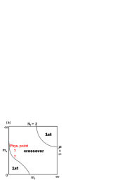
For higher , the chiral crossover at the physical point is expected to become first order. In this case, there appears a critical end point (CEP) of the first-order transition line, and the transition becomes second order on CEP Asakawa and Yazaki (1989); Barducci et al. (2006); Kashiwa et al (2006). However, clear evidence of the behavior is not shown yet by LQCD because of the sign problem at real .
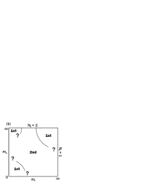
On the contrary, LQCD is feasible Forcrand and Philipsen (2002); D’Elia and Lombardo (2003); Chen and Luo (2005, 2005); D’Elia et al (2009); Cea et al. (2009); D’Elia et al (2009); FP2010 (2009); Nagata et al (2009); Takaishi et al (2010) at imaginary , where stands for the temperature and represents the dimensionless chemical potential. QCD has a periodicity of in called the Roberge-Weiss (RW) periodicity Roberge and Weiss (1986), because QCD is invariant under the extended transformation Sakai et al (2008). At mod , there appears a first-order transition at higher than some temperature Roberge and Weiss (1986). This is now called the RW transition Roberge and Weiss (1986). On the RW transition line starting from the end point , a spontaneous symmetry breaking occurs Kouno et al (2009). Very recently, the order of the symmetry breaking at the RW end point has been analyzed by two-flavor D’Elia et al (2009) and degenerate three-flavor FP2010 (2009) LQCD. For the two cases, the order is first order at small and large quark masses, but second order for intermediate masses. Figure 1(b) is a sketch based on the LQCD results for the RW phase transition at the end point . Most of the region is unknown at the present stage.
As an approach complementary to first-principle LQCD, we can consider effective models such as the Nambu–Jona-Lasinio (NJL) model Asakawa and Yazaki (1989); Kashiwa et al (2006); Reinberg and the Polyakov-loop extended Nambu–Jona-Lasinio (PNJL) model Kouno et al (2009); Sakai et al (2008); Meisinger et al. (1996); Fukushima (2004); Ratti et al. (2006); Rossner et al. (2007); Schaefer (2007); Kashiwa et al (2008); Sakai et al (2008); Kasihwa et al (2009); Matsumoto (2010); Sasaki et al. (2009); Sakai (2010); Gatto (2011). The NJL model can describe the chiral symmetry breaking, but not the confinement mechanism. The PNJL model is designed to make it possible to treat both the mechanisms. The effective models have ambiguity in determining their parameters Kasihwa et al (2009); Sakai et al (2008); Matsumoto (2010). We then take the following strategy. We first construct an effective model and determine parameters of the model in the regions where LQCD is feasible. Next, we predict physical quantities in the regions where LQCD is not feasible, using the constructed model.
The original PNJL model cannot reproduce LQCD data at imaginary quantitatively Sakai et al (2008). This shortcoming of the PNJL model seems to be originated in the fact that the correlation between the chiral condensate and the Polyakov loop is too weak. Therefore, in Ref. Sakai (2010), we extended the two-flavor PNJL model by introducing the effective four-quark vertex depending on . This effective vertex includes additional mixing effects between and . The new model is called the entanglement PNJL (EPNJL) model. The two-flavor EPNJL model reproduces LQCD data at zero and imaginary , particularly on strong correlations between the chiral and deconfinement transitions and also on quark-mass dependence of the order of the RW end point D’Elia et al (2009). The two-flavor EPNJL model reproduces all LQCD data, without changing the parameters, at small real without Sakai (2010) and with strong magnetic field Gatto (2011) and at finite isospin chemical potential Sakai (2010).
In this paper, we extend the two-flavor EPNJL model to the three-flavor case. Parameters of the three-flavor EPNJL model are determined from LQCD data at zero and at the RW end point. The Columbia pot is drawn for the chiral transition at zero and for the symmetry breaking at the RW end point.
Model setting. We start with the three-flavor PNJL model. The Lagrangian density of the model is
| (1) |
where with the gauge coupling and the Gell-Mann matrices . Three-flavor quark fields have current quark masses . In the interaction part, and denote coupling constants of the scalar-type four-quark and the Kobayashi-Maskawa-’t Hooft (KMT) determinant interaction Kobayashi and Maskawa (1970); ’t Hooft (1976), respectively, in which the determinant runs in the flavor space. The KMT determinant interaction breaks the symmetry explicitly.
In the PNJL model, the gauge field is treated as a homogeneous and static background field Fukushima (2004). The Polyakov loop and its conjugate are determined in the Euclidean space by
| (2) |
where with . In the Polyakov gauge, is diagonal in the color space. The Polyakov potential is assumed to be a function of and . We take the Polyakov potential of Ref. Rossner et al. (2007):
| (3) | |||
| (4) |
Parameters of are determined to reproduce LQCD data at finite in the pure gauge limit.
Using the mean field approximation to the quark-quark interactions in (1), one can get the thermodynamic potential (per volume) Matsumoto (2010):
| (5) |
where and for . The dynamical quark mass is defined by
| (6) |
for . The variables , , and are determined by the stationary condition Matsumoto (2010).
When , the thermodynamic potential of QCD has the RW periodicity Roberge and Weiss (1986), i.e. a periodicity of in . The PNJL thermodynamic potential of (5) also has this periodicity, since the potential is invariant under the extended transformation Sakai et al (2008). At and , is symmetric Kouno et al (2009). Particularly at , it is spontaneously broken at higher Roberge and Weiss (1986); Kouno et al (2009). The order parameter of the spontaneous symmetry breaking is a -odd quantity such as the imaginary part of the modified Polyakov loop Kouno et al (2009).
An origin of the four-quark vertex is a gluon exchange between quarks and its higher-order diagrams. If the gluon field has a vacuum expectation value in its time component, is coupled to that is related to through Kondo (2010). Hence, is changed into an effective vertex depending on Kondo (2010). Here, the effective vertex is called the entanglement vertex and all interactions including are referred to as the entanglement interactions. It is expected that dependence of will be determined in the future by the accurate method such as the exact renormalization group method Braun (2010); Kondo (2010); Wetterich (1993). In this paper, however, we simply assume the following that preserves the chiral symmetry, the symmetry Kouno et al (2009) and the extended symmetry Sakai et al (2008):
| (7) |
This modification changes the mesonic terms having and the dynamical quark masses in . This is the three-flavor version of the EPNJL model, and this model has entanglement interactions in and in addition to the covariant derivative included in the original PNJL model. In principle, can depend on , too. However, we found that the dependence of yields qualitatively the same effect on the phase diagram as that of . As a simple setup, we then neglect the dependence of . In the present analysis, thus, the -dependence of is renormalized in that of .
In the thermodynamic potential (5), we impose the isospin symmetry for the - sector () and take the three-dimensional cutoff for the momentum integration Matsumoto (2010), because this model is nonrenormalizable. Hence, the three-flavor PNJL model has five parameters , , , , and . We use the parameter set of Table 1 Reinberg . These parameters are fitted to reproduce empirical values of -meson mass and decay constant, -meson mass and decay constant and meson mass at vacuum.
| 5.5 | 140.7 | 602.3 | 1.835 | 12.36 |
Parameters of are determined to reproduce LQCD data at finite in the pure gauge limit Rossner et al. (2007). The original value of is 270 MeV, but the deconfinement temperature determined by the EPNJL model with this value of is much larger than MeV predicted by full LQCD Borsanyi etal (2010); Soeldner (2010); Kanaya (2010). Therefore, we rescale to 150 MeV so that the EPNJL model can reproduce MeV.
The parameters and in (7) are so determined as to reproduce two results of LQCD at finite . The first is a result of 2+1 flavor LQCD at YAoki that the chiral transition is crossover at the physical point. The second is a result of degenerate three-flavor LQCD at FP2010 (2009) that the order of the RW end point is first order for small and large quark masses but second order for intermediate quark masses. The parameter set satisfying these conditions is located in the triangle region
| (8) |
Here, we take as a typical example.
Results. Figure 2 shows dependence of light- and strange-quark condensates, and , and the Polyakov loop at . In the PNJL model of panel (a), and rapidly decrease at MeV as increases, after rapidly increases at MeV as increases. Thus, the pseudocritical temperature of the chiral crossover is much higher than that of the deconfinement crossover. The same property is also seen in the two-flavor case Sakai et al (2008). In the EPNJL model of panel (b), meanwhile, the pseudocritical temperatures of the chiral and the deconfinement crossover almost coincide at MeV.
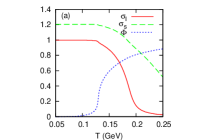

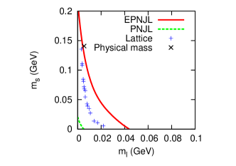
Figure 3 shows the order of the chiral transition in the - plane at . This figure corresponds to the small and part of Fig.1(a). The second-order chiral-transition line is drawn for three cases, the PNJL result (dotted line) and the EPNJL result (solid line) and LQCD data (+ symbols) Forcrand and Philipsen (2002). For each of the three cases, there are the first-order region below the second-order line and the crossover region above the line. The second-order line predicted by the EPNJL model is close to that by LQCD data particularly near the physical point. Meanwhile, the first-order region predicted by the PNJL model is much smaller than that by LQCD data. Thus, the EPNJL model yields much better agreement with LQCD prediction than the PNJL model.
The deconfinement transitions predicted by the PNJL and EPNJL models are crossover in the whole region shown in Fig. 3. In the EPNJL model, the crossover deconfinement transition almost coincides with the chiral transition, even if the chiral transition is crossover.
Now we consider the symmetry breaking at for the case of three degenerate flavors (). Figure 4 represents the imaginary part of as a function of and predicted by the three-flavor EPNJL model. When is large, the system is close to the pure gauge limit and hence the -symmetry breaking is first order. When is small, meanwhile, the system is nearly chirally symmetric and therefore the transition is first order. In the intermediate mass region, the transition is second order. The result is consistent with the LQCD data FP2010 (2009).
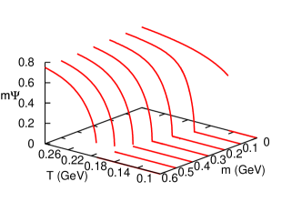
Figure 5 shows the phase diagram for the -symmetry breaking at the RW end point predicted by the EPNJL model. The diagram is plotted as a function of and up to , the upper limit for the present model to be applicable. The two solid lines represent boundaries between the first- and second-order transition regions. Below (above) the lower (upper) boundary, the transition is first order. The dotted line of corresponds to the case of . On the dotted line, the order is first order for small and large masses but second order for intermediate masses, as expected. At the physical point, the order is second order for the present parameter set. However, the order can becomes first order at the physical point, if we take other parameter sets belonging to the region (8). In the PNJL model, meanwhile, the transition is always first order in the entire region of the - plane.
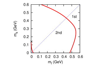
In Figs. 4 and 5, the EPNJL prediction is shown for small and large current quark masses (). The applicability of the NJL-type model to large , however, is an open question. In fact it was pointed out that dependence of the chiral-transition temperature is not consistent with the corresponding LQCD results Dumitru (2004); Braun2 (2006); as increases, the chiral-transition temperature goes up sizably in the NJL-type model but hardly changes in the LQCD results. In the EPNJL model, the chiral-transition temperature almost coincides with the deconfinement one that hardly depends on , so that the EPNJL result is consistent with the LQCD result for the transition temperature. It was also pointed out that for large the pion mass calculated with the NJL-type model is larger than the corresponding LQCD result Kahara (2009). In the NJL-type model the hadron mass calculation is questionable for large , particularly when the calculated hadron mass is bigger than the cutoff . Therefore, the ENJL predictions shown in Fig. 4 and 5 should be regarded as qualitative ones for the MeV region where the calculated pion mass is bigger than . However, the fact that there is the second-order region at intermediate (MeV) shows that there exists a boundary between the first- and second-order regions at large . In this qualitative sense, the phase diagram of Fig. 5 is reasonable for large .
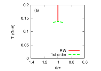
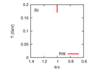
Figure 6 presents the phase diagram in the - plane predicted by the PNJL and EPNJL models, where and have physical values. In the PNJL model of panel (a), a first-order RW transition (solid) line is connected at the RW end point to two first-order deconfinement (dashed) lines. Hence, the RW end point is a triple point. In the EPNJL model of panel (b), the RW transition is second order at the end point, so that there is no first-order deconfinement line connected to the first-order RW transition line. For other parameter sets in the parameter region (8), the transition is weak first-order at the end point and hence the first-order RW transition line is connected at the RW end point to two very-short first-order deconfinement lines.
Summary. In summary, we have extended the three-flavor PNJL model by introducing an entanglement vertex . The entanglement PNJL (EPNJL) model is consistent with 2+1 flavor LQCD data for the chiral transition at and degenerate three-flavor LQCD data for the RW transition at the end point calculated very lately. The three-flavor phase diagram for the RW transition at the end point is first drawn in the - plane by the EPNJL model justified above.
Acknowledgements.
The authors thank A. Nakamura, T. Saito, K. Nagata, and K. Kashiwa for useful discussions. H.K. also thanks M. Imachi, H. Yoneyama, H. Aoki, and M. Tachibana for useful discussions. T.S and Y.S. are supported by JSPS.References
- (1) Y. Aoki, G. Endrödi, Z. Fodor, S. D. Katz and K. K. Szabó, Nature 443, 675 (2006).
- Borsanyi etal (2010) S. Borsányi, Z. Fodor, C. Hoelbling, S. D. Katz, S. Krieg, C. Ratti, and K. K. Szabo, arXiv:1005.3508 [hep-lat] (2010).
- Soeldner (2010) W. Söldner, arXiv:1012.4484 [hep-lat] (2010).
- Kanaya (2010) K. Kanaya, arXiv:hep-ph/1012.4235 [hep-ph] (2010); arXiv:hep-ph/1012.4247 [hep-lat] (2010).
- (5) E. Laermann and O. Philipsen, Ann. Rev. Nucl. Part. Sci. 53, 163 (2003);
- Forcrand and Philipsen (2002) P. de Forcrand and O. Philipsen, J. High Energy Phys. 01, 077 (2007).
- Asakawa and Yazaki (1989) M. Asakawa and K. Yazaki, Nucl. Phys. A504, 668 (1989).
- Kashiwa et al (2006) K. Kashiwa, H. Kouno, T. Sakaguchi, M. Matsuzaki, and M. Yahiro, Phys. Lett. B 647, 446 (2007); K. Kashiwa, M. Matsuzaki, H. Kouno, and M. Yahiro, Phys. Lett. B 657, 143 (2007).
- Barducci et al. (2006) A. Barducci, R. Casalbuoni, S. De Curtis, R. Gatto, and G. Pettini, Phys. Lett. B 231, 463 (1989); A. Barducci, R. Casalbuoni, G. Pettini, and R. Gatto, Phys. Rev. D 49, 426 (1994);
- Forcrand and Philipsen (2002) P. de Forcrand and O. Philipsen, Nucl. Phys. B642, 290 (2002); P. de Forcrand and O. Philipsen, Nucl. Phys. B673, 170 (2003).
- D’Elia and Lombardo (2003) M. D’Elia and M. P. Lombardo, Phys. Rev. D 67, 014505 (2003); Phys. Rev. D 70, 074509 (2004); M. D’Elia, F. D. Renzo, and M. P. Lombardo, Phys. Rev. D 76, 114509 (2007);
- Chen and Luo (2005) H. S. Chen and X. Q. Luo, Phys. Rev. D72, 034504 (2005); arXiv:hep-lat/0702025 (2007).
- Chen and Luo (2005) L. K. Wu, X. Q. Luo, and H. S. Chen, Phys. Rev. D76, 034505 (2007).
- D’Elia et al (2009) M. D’Elia and F. Sanfilippo, Phys. Rev. D 80, 014502 (2009).
- Cea et al. (2009) P. Cea, L. Cosmai, M. D’Elia, C. Manneschi and A. Papa, Phys. Rev. D 80, 034501 (2009).
- D’Elia et al (2009) M. D’Elia and F. Sanfilippo, Phys. Rev. D 80, 111501 (2009).
- FP2010 (2009) P. de Forcrand and O. Philipsen, arXiv:1004.3144 [hep-lat](2010).
- Nagata et al (2009) K. Nagata, A. Nakamura, Y. Nakagawa, S. Motoki, T. Saito and M. Hamada, arXiv:0911.4164 [hep-lat](2009); K. Nagata, and A Nakamura, arXiv:1104.2142 [hep-ph] (2011).
- Takaishi et al (2010) T. Takaishi, P. de Forcrand and A. Nakamura, arXiv:1002.0890 [hep-lat](2010).
- Roberge and Weiss (1986) A. Roberge and N. Weiss, Nucl. Phys. B275, 734 (1986).
- Sakai et al (2008) Y. Sakai, K. Kashiwa, H. Kouno, and M. Yahiro, Phys. Rev. D 77, 051901(R) (2008); Phys. Rev. D 78, 036001 (2008); Y. Sakai, K. Kashiwa, H. Kouno, M. Matsuzaki, and M. Yahiro, Phys. Rev. D 78, 076007 (2008); K. Kashiwa, M. Matsuzaki, H. Kouno, Y. Sakai, and M. Yahiro, Phys. Rev. D 79, 076008 (2009); K. Kashiwa, H. Kouno, and M. Yahiro, Phys. Rev. D 80, 117901 (2009).
- Kouno et al (2009) H. Kouno, Y. Sakai, K. Kashiwa, and M. Yahiro, J. Phys. G: Nucl. Part. Phys. 36, 115010 (2009); H. Kouno, Y. Sakai, T. Sasaki, K. Kashiwa, and M. Yahiro, Phys. Rev. D 83, 076009 (2011).
- (23) P. Reinberg, S.P. Klevansky and J. Hüfner, Phys. Rev. C 53, 410 (1996); S.P. Klevansky, Rev. Mod. Phys. 64, 649 (1992).
- Meisinger et al. (1996) P. N. Meisinger, and M. C. Ogilvie, Phys. Lett. B 379, 163 (1996).
- Fukushima (2004) K. Fukushima, Phys. Lett. B 591, 277 (2004); Phys. Rev. D 77, 114028 (2008).
- Ratti et al. (2006) C. Ratti, M. A. Thaler, and W. Weise, Phys. Rev. D 73, 014019 (2006).
- Rossner et al. (2007) S. Rößner, C. Ratti, and W. Weise, Phys. Rev. D 75, 034007 (2007).
- Schaefer (2007) B. -J. Schaefer, J. M. Pawlowski, and J. Wambach, Phys. Rev. D 76, 074023 (2007).
- Kashiwa et al (2008) K. Kashiwa, H. Kouno, M. Matsuzaki, and M. Yahiro, Phys. Lett. B 662, 26 (2008).
- Sakai et al (2008) Y. Sakai, K. Kashiwa, H. Kouno, M. Matsuzaki, and M. Yahiro, Phys. Rev. D 79, 096001 (2009);
- Kasihwa et al (2009) K. Kashiwa, M. Yahiro, H. Kouno, M. Matsuzaki, and Y. Sakai, J. Phys. G: Nucl. Part. Phys. 36, 105001 (2009).
- Matsumoto (2010) T. Matsumoto, K. Kashiwa, H. Kouno, K. Oda, and M. Yahiro, Phys. Lett. B 694, 367 (2011).
- Sasaki et al. (2009) T. Sasaki, Y. Sakai, H. Kouno, and M. Yahiro, Phys. Rev. D 82, 116004 (2010); Y. Sakai, H. Kouno, and M. Yahiro, J. Phys. G: Nucl. Part. Phys. 37, 105007 (2010); Y. Sakai, T. Sasaki, H. Kouno, and M. Yahiro, Phys. Rev. D 82, 096007 (2010).
- Sakai (2010) Y. Sakai, T. Sasaki, H. Kouno, and M. Yahiro, Phys. Rev. D 82, 076003 (2010); arXiv:1104.2394 [hep-ph] (2011).
- Gatto (2011) R. Gatto, and M. Ruggieri, Phys. Rev. D 83, 034016 (2011).
- Kobayashi and Maskawa (1970) M. Kobayashi, and T. Maskawa, Prog. Theor. Phys. 44, 1422 (1970); M. Kobayashi, H. Kondo, and T. Maskawa, Prog. Theor. Phys. 45, 1955 (1971).
- ’t Hooft (1976) G. ’t Hooft, Phys. Rev. Lett. 37, 8 (1976); Phys. Rev. D 14, 3432 (1976); 18, 2199(E) (1978).
- Kondo (2010) K.-I. Kondo, Phys. Rev. D 82, 065024 (2010).
- Braun (2010) J. Braun, L. M. Haas, F. Marhauser, and J. M. Pawlowski, Phys. Rev. Lett. 106, 022002 (2011); J. Braun, and A. Janot, arXiv:1102.4841 [hep-ph] (2011).
- Wetterich (1993) C. Wetterich, Phys. Lett. B 301, 90 (1991).
- Dumitru (2004) A. Dumitru, D. Röder, and J. Ruppert, Phys. Rev. D 70, 074001 (2004).
- Braun2 (2006) J. Braun, B. Klein, H.-J. Pirner, and A.H. Rezaeian, Phys. Rev. D 73, 074010 (2006).
- Kahara (2009) T. Kähärä, and K. Tuominen, Phys. Rev. D 80, 114022 (2009).