The Structure of 2MASS Galaxy Clusters

Abstract

We use a sample of galaxies from the Two Micron All Sky Survey (2MASS) Extended Source Catalog to refine a matched filter method of finding galaxy clusters that takes into account each galaxy’s position, magnitude, and redshift if available. The matched filter postulates a radial density profile, luminosity function, and line-of-sight velocity distribution for cluster galaxies. We use this method to search for clusters in the galaxy catalog, which is complete to an extinction-corrected $K$-band magnitude of $13.25$ and has spectroscopic redshifts for roughly 40% of the galaxies, including nearly all brighter than $K=11.25$. We then use a stacking analysis to determine the average luminosity function, radial distribution, and velocity distribution of cluster galaxies in several richness classes, and use the results to update the parameters of the matched filter before repeating the cluster search. We also investigate the correlations between a cluster’s richness and its velocity dispersion and core radius, using these relations to refine priors that are applied during the cluster search process. After the second cluster search iteration, we repeat the stacking analysis. We find a cluster galaxy luminosity function that fits a Schechter form, with parameters $M_{K*}-5\log h=-23.64\pm 0.04$ and $\alpha=-1.07\pm 0.03$. We can achieve a slightly better fit to our luminosity function by adding a Gaussian component on the bright end to represent the brightest cluster galaxy (BCG) population. The radial number density profile of galaxies closely matches a projected Navarro-Frenk-White (NFW) profile at intermediate radii, with deviations at small radii due to well-known cluster centering issues and outside the virial radius due to correlated structure. The velocity distributions are Gaussian in shape, with velocity dispersions that correlate strongly with richness.

1. Introduction

As the most massive structures known that are in dynamical equilibrium, clusters of galaxies are useful for studies of large-scale structure (e.g., Bahcall, 1988; Einasto et al., 2001; Yang et al., 2005; Papovich, 2008), as well as for galaxy formation and evolution (e.g., Dressler & Gunn, 1992; Goto et al., 2003) and for constraining cosmological parameters (e.g., Henry, 2000; Allen et al., 2008; Rozo et al., 2010). The problem of finding clusters of galaxies has been attacked from several angles. The oldest method is simply to look for overdensities in the two-dimensional distribution of galaxies on the sky (e.g., Abell, 1958; Zwicky et al., 1968; Abell et al., 1989). This method faces difficulties caused by line-of-sight interlopers, a problem which has been greatly ameliorated in recent years by photometric (so-called 2.5-dimensional) and spectroscopic redshift surveys. Several algorithms have been used to analyze such data, including the percolation (or friends-of-friends) algorithm (e.g., Huchra & Geller, 1982; Crook et al., 2007), the red sequence method (e.g., Gladders & Yee, 2000; Koester et al., 2007) and the matched filter method (e.g., Postman et al., 1996; Kepner et al., 1999; Kochanek et al., 2003; Dong et al., 2008; Szabo et al., 2011). Other fruitful strategies include searching for the thermal X-ray emission of the hot intra-cluster gas (e.g., Gioia et al., 1990; Ebeling et al., 1998; Böhringer et al., 2001; Mullis et al., 2003) and searching for the weak lensing signature of clusters (e.g., Schneider, 1996; Wittman et al., 2001; Sheldon et al., 2009). The most recently developed approach is to search for the thermal Sunyaev-Zeldovich decrement in the cosmic microwave background caused by this same gas (e.g., Carlstrom et al., 2000; LaRoque et al., 2003; Staniszewski et al., 2009). These methods can be used to estimate cluster masses, which are important for comparison with theory. But optical and infrared (IR) surveys primarily measure cluster richness, a quantity which, though correlated with cluster mass, has significant scatter at fixed mass.

In this paper we follow up the work of Kochanek et al. (2003, K03 hereafter), who use a matched filter algorithm based largely on the earlier approach of Kepner et al. (1999) to find clusters of galaxies in the Two Micron All Sky Survey (2MASS) Extended Source Catalog (Jarrett et al., 2000; Skrutskie et al., 2006). This method makes use of the expected properties of galaxy clusters — specifically, their shapes in angular and redshift space, and the luminosity function of their members. Our aim in this paper is to evaluate and update the parameters of the matched filter in order to increase the completeness and purity of the resulting cluster catalog, and to obtain richness estimates that are as accurate as possible. The large number of clusters in the 2MASS catalog enable us to use a stacking analysis to find their average properties. We use an iterative strategy: first, we search for clusters using a filter very similar to that of K03, then we stack the resulting clusters to determine their average radial density profile, velocity distribution, and luminosity function as a function of richness. Using these properties, we then refine the matched filter and repeat the cluster search and stacking analysis, adopting the results of this second iteration as our best estimate of the average properties of the cluster sample. Throughout this work we refer to these as the first and second cluster search iterations.

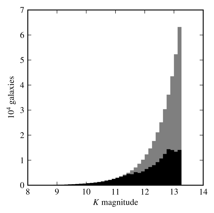
Figure 1.— Apparent magnitude distribution of all input galaxies (gray) and input galaxies with spectroscopic redshift measurements (black).

K03 used a few modifications to their likelihood function to stabilize parameter estimation and reflect prior knowledge; we incorporate and expand these. In particular, one set of priors makes use of the relationship between a cluster’s richness and its core radius and velocity dispersion. Since our cluster search method produces estimates of these quantities for each cluster, we use the correlations we observe in the first cluster search iteration to tune this set of priors for the second iteration.

We use a deeper version of the galaxy catalog used by K03: a flux-limited selection from the 2MASS Extended Source Catalog with $K<13.25$ and Galactic latitudes $|b|>6^{\circ}$. The $20$ mag arcsec^-1 isophotal $K$-band magnitudes are corrected for Galactic extinction using the Schlegel et al. (1998) extinction model. Of our sample of 380360 galaxies, 161030 have spectroscopic redshifts from a preliminary version of 2MASS Redshift Survey (2MRS, Huchra et al., 2011). The 2MRS contains not only redshifts measured by Huchra et al. (2011), but also compiles redshifts from many other sources. Out of about 950, some of the most important contributors are the Six-degree Field Galaxy Redshift Survey (e.g., Jones et al., 2004), the Sloan Digital Sky Survey (e.g., Abazajian et al., 2005), the Two-degree Field Galaxy Redshift Survey (e.g., Colless et al., 2001), the Center for Astrophysics Redshift Survey (e.g., Huchra et al., 1983; Falco et al., 1999), the Las Campanas Redshift Survey (LCRS, Shectman et al., 1996), the ESO Nearby Abell Cluster Survey (Katgert et al., 1998), the Southern Sky Redshift Survey (da Costa et al., 1998), and others (e.g., Bottinelli et al., 1990; Loveday et al., 1996). The complete list of sources is given by Huchra et al. (2011). Essentially all of the 23046 galaxies with $K<11.25$ have redshift measurements, as do 138157 galaxies fainter than that limit. The apparent magnitude distribution of our galaxy sample is shown in Figure 1. In our second cluster search iteration, we find 7624 cluster candidates that exceed our likelihood threshold, most with redshifts below $0.1$. The clusters are essentially characterized by the intrinsic richness $N_{*}$, as well as by an “apparent richness” $N_{g}$, which declines with distance as galaxies below the apparent magnitude limit drop out of the galaxy catalog. We show the distribution of the cluster candidates in redshift and richness in Figure 2. Together with the likelihood values of individual clusters, the completeness and purity of the cluster catalog decline as $N_{g}$ decreases. They, as well as mass estimates and comparisons to other cluster surveys, are the subject of a forthcoming paper.

In Section 2 we describe our galaxy cluster model, which includes the spatial and velocity distribution of cluster galaxies and their luminosity function. We use this model as a matched filter to find clusters. In Section 3 we describe the stacking technique with which we determine the average properties of the clusters in order to update the model. In Section 4 we describe the priors that we use the modify the likelihood function, and use the initial sample of clusters to update some of their parameters. Finally, in Section 5 we conclude. The work described in K03 used a cosmological model with $\Omega_{M}=1$ and $\Omega_{\Lambda}=0$. The details of the cosmological model are not very important for our purposes since the 2MASS galaxies are nearby, but for this work we use a cosmology with $\Omega_{M}=0.3$ and $\Omega_{\Lambda}=0.7$. We use the usual parameterization for the Hubble constant, with $H_{0}=100h~{}\mathrm{km}~{}\mathrm{s}^{-1}~{}\mathrm{Mpc}^{-1}$.

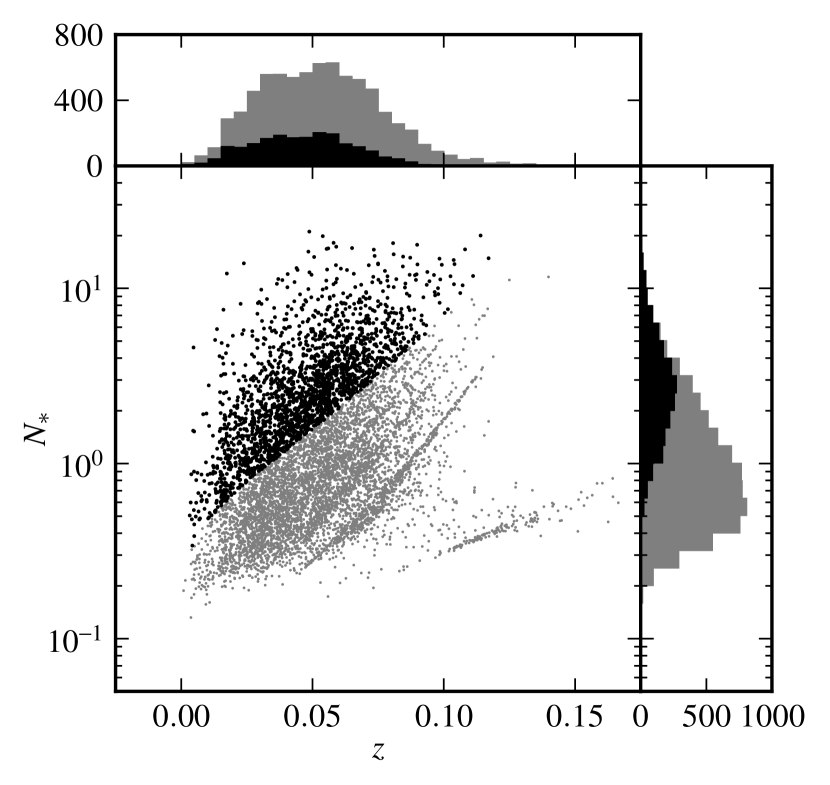
Figure 2.— Richness $N_{*}$ and redshift $z$ of the cluster candidates resulting from our second cluster search iteration. The black points are those clusters for which $N_{*666}>3$, a sample which K03 found to be highly pure. The black histograms correspond to these clusters, while the gray histograms represent all clusters with $\Delta\ln\mathcal{L}\geq 5$. The search is deliberately extended to low $\Delta\ln\mathcal{L}$ and $N_{*}$ to allow for later investigation of false positives.

2. The Matched Filter Method

Following the method of Kepner et al. (1999) as expanded by K03, we search for clusters by computing a likelihood which is the convolution of the observed distribution of galaxies (in angular, redshift, and luminosity space) with a filter tuned to match the “shape” of galaxy clusters. This convolution smooths out the small-scale details of individual galaxy locations but maximizes the signal due to actual cluster-shaped galaxy overdensities. This method has several advantages. It provides estimates for the likelihood of each detected cluster, as well as for the membership probabilities of each nearby galaxy. In its K03 realization, it also provides best-fit values and uncertainties for cluster properties such as richness and velocity dispersion, and it is flexible enough to handle galaxies with or without redshift and color information; this is important for our sample, where not every galaxy has a redshift measurement.

2.1. The Cluster Model

We add clusters to the catalog in an iterative fashion, at each step evaluating the likelihood function at the position of each galaxy in the sample and adding a cluster centered on the galaxy with the highest likelihood. The likelihood function is constructed from the probabilities of the nearby galaxies to be cluster members or non-member field galaxies; these probabilities make up the matched filter. For a proposed $n_{c}$-th galaxy cluster, the change in likelihood is

$$\Delta\ln\mathcal{L}(n_{c})=-N_{*n_{c}}A_{n_{c}}+\sum_{i}\ln\left[\frac{P_{f}(i)+\sum_{k=1}^{n_{c}}P_{c}(i,k)}{P_{f}(i)+\sum_{k=1}^{n_{c}-1}P_{c}(i,k)}\right]~{},$$ (1)

where the sum in $i$ is over all galaxies within the sampling radius $R_{\mathrm{samp}}=1.0\,h^{-1}$ Mpc. The term $-N_{*n_{c}}A_{n_{c}}$ is an estimate of the total number of member galaxies we expect to be visible within $R\leq R_{\mathrm{samp}}$ of the proposed cluster, given the survey magnitude limit; we give an expression for it in Equation (14). The definitions of $P_{f}$ and $P_{c}$ are given in Equations (2) and (2.1), respectively. The expression for the likelihood in Equation (1) is derived in Appendix C2 of Kepner et al. (1999). The likelihood depends on the richness, redshift, core radius, and velocity dispersion of the candidate cluster, mostly through $P_{c}$; we optimized these values using the Markov Chain Monte Carlo (MCMC) method while evaluating the likelihood. The clusters labeled $k=1\cdots n_{c}-1$ are already in the cluster catalog, and have fixed properties. We account for previously found clusters via their inclusion in the denominator of the last term in the equation; this effectively removes them from the density field in a manner similar to the Clean algorithm of radio astronomy (Högbom, 1974). We stop iterating when no cluster is found that increases the likelihood by more than a predetermined cutoff value. We choose $\Delta\ln\mathcal{L}=5$ as our cutoff; this is low enough that most of the low-likelihood cluster candidates are in fact false positives (see K03). In Section 3 we select a relatively pure subset of clusters for analysis, all of which have likelihoods well above the cutoff. The likelihood of a given cluster correlates well with $N_{g}$, the number of member galaxies brighter than the survey limit, and only weakly with the actual richness $N_{*}$.

The probability of finding a field galaxy with a given absolute $K$ magnitude $M_{K}$ and redshift $z$ in some infinitesimal portion of the sky is

$$P_{f}=0.4\ln(10)D_{C}^{2}(z)\frac{dD_{C}}{dz}\phi_{f}(M_{K})~{},$$ (2)

where $D_{C}$ is the comoving distance and $\phi_{f}$ is the field galaxy luminosity function. When the redshift of the galaxy is not known, we average $P_{f}$ over the range $0\leq z<1$; this is effectively the differential number count of the 2MASS survey. We follow K03 in adopting the luminosity function of Kochanek et al. (2001) for $\phi_{f}$. It is a Schechter function (Schechter, 1976), with parameters $M_{K*}=-23.39$ and $\alpha=-1.09$, and normalization $n_{*}=1.16\times 10^{-2}h^{3}$ Mpc^-3. We also use this luminosity function for cluster galaxies in our first search iteration; see Equation (5). In the second iteration we update the cluster luminosity function, but the field luminosity function stays unchanged. Following the example of K03, we calculate the absolute magnitudes using an effective distance modulus

$$\mathcal{D}(z)=K-M_{K}\equiv 5\log(D_{L}(z)/10~{}\mathrm{pc})+k(z)$$ (3)

that includes a $k$-correction $k(z)=-6\log(1+z)$ in addition to the term containing the luminosity distance $D_{L}(z)$. As K03 note, this $k$-correction is negative, independent of galaxy type, and valid for $z\lesssim 0.25$. Due to our parameterization of Hubble’s constant, we report values of $M_{K}-5\log h$, but hereafter we omit the second term for the sake of brevity.

The model for the distribution of galaxies with absolute $K$-band magnitudes $M_{K}$, projected radii $R$, and measured redshifts $z$ relative to a cluster at redshift $z_{c}$ with richness $N_{*}$, velocity dispersion $\sigma_{c}$, and scale radius $r_{c}$ (or alternatively, the probability of the cluster having a member galaxy with these characteristics) is

$$P_{c} =\frac{dN}{d^{2}xdM_{K}dz}$$

$$=N_{*}\frac{\phi_{c}(M_{K})}{\Phi_{c}(M_{K*})}\frac{\Sigma(R)}{\sqrt{2\pi}\sigma_{c}(1+z_{c})}\exp\left[-\frac{c^{2}(z-z_{c})^{2}}{2\sigma_{c}^{2}(1+z_{c})^{2}}\right]~{}.$$ (4)

The normalization $N_{*}$ is the number of cluster galaxies brighter than $M_{K*}$ within a spherical radius $r_{\mathrm{out}}$ of the cluster center. This radius ought to be roughly similar to the virial radius. Like most previous matched filter studies, we choose $r_{\mathrm{out}}=1.0\,h^{-1}$ Mpc. Using a fixed physical radius is convenient for calculations, and avoids adding extra scatter to richness estimates via the use of a noisy virial radius estimate. We discuss other possible richness measures in Section 2.2. The integrated luminosity function $\Phi_{c}(M_{K})$ is the spatial density of galaxies brighter than $M_{K}$, and is the cumulative integral of the cluster luminosity function $\phi_{c}(M_{K})$. The function $\Sigma(R)$ represents the two-dimensional spatial distribution of galaxies, and is given by a projected version of the Navarro-Frenk-White (NFW, Navarro et al., 1997) profile. Finally, the Gaussian factor in redshift $z$ represents the line of sight velocity distribution of the cluster galaxies. We describe these components in greater detail in the following paragraphs.

The luminosity function of cluster galaxies is assumed to be given by a Schechter function with fixed parameters $\alpha$ and $M_{K*}$,

$$\phi_{c}(M_{K})=0.4\ln(10)n_{*}\left(\frac{L_{K}}{L_{K*}}\right)^{1+\alpha}\exp\left(-\frac{L_{K}}{L_{K*}}\right)~{},$$ (5)

where $M_{K}-M_{K*}=-2.5\log(L_{K}/L_{K*})$. The integrated luminosity function, which describes the density of cluster galaxies brighter than a specified magnitude, is thus the incomplete Gamma function

$$\Phi_{c}(M_{K})=\int_{-\infty}^{M_{K}}\phi_{c}(M)dM=n_{*}\Gamma\left(1+\alpha,\frac{L_{K}}{L_{K*}}\right)~{}.$$ (6)

Since $\phi_{c}$ only appears in our calculations as a fraction of $\Phi_{c}$, its normalization constant $n_{*}$ is unimportant. For our first cluster finding iteration, we follow K03 in adopting the Kochanek et al. (2001) luminosity function and set $\alpha$ and $M_{K*}$ to $-1.09$ and $-23.39$ mags, respectively. Part of the purpose of this work is to verify the appropriateness of this choice for the cluster galaxy luminosity function, and we update these parameter values in our second iteration.

We model the angular distribution of cluster galaxies as the two-dimensional projection of an NFW profile. For a cluster with a scale radius $r_{c}$, this distribution, normalized by the number of galaxies within an outer radius $Cr_{c}$, is given in three dimensions by

$$\rho(r)=\frac{1}{4\pi r_{c}^{3}F(C)}\frac{1}{x(1+x)^{2}}~{},$$ (7)

where $x=r/r_{c}$ and $F(x)=\ln(1+x)-x/(1+x)$. The parameter $C$ is similar to the concentration of the cluster. For the purpose of normalizing this profile (or equivalently, defining $N_{*}$), we fix it to $C=(1.0\,h^{-1}\,\mathrm{Mpc})/r_{c}$. The projected profile is

$$\Sigma(R)=\frac{f(R/r_{c})}{2\pi r_{c}^{2}F(C)}~{},$$ (8)

where

$$f(x)=\frac{1}{x^{2}-1}\left[1-\frac{2}{(x^{2}-1)^{1/2}}\tan^{-1}\left(\frac{x-1}{x+1}\right)^{1/2}\right]$$ (9)

and for $x<1$ we use the identity $-i\tan^{-1}(ix)=\tanh^{-1}(x)$. Finally, the number of galaxies enclosed within a circular radius $R$ is given by $N(<R)=g(R/r_{c})/F(C)$, where

$$g(x)=\ln\left(\frac{x}{2}\right)+\frac{2}{(x^{2}-1)^{1/2}}\tan^{-1}\left(\frac{x-1}{x+1}\right)^{1/2}$$ (10)

(Bartelmann, 1996). Apart from its normalization, this density profile model has a single parameter: the core radius $r_{c}$. We allow it to vary when calculating likelihoods in order to maximize the likelihood (subject to some priors; see Section 4). The “concentration” parameter $C$ varies with it, being defined as $(1.0\,h^{-1}\,\mathrm{Mpc})/r_{c}$. This is in contrast to K03, who fix $r_{c}$ and $C$ to values of $0.2\,h^{-1}$ Mpc and $4$, respectively.

The final factor in the cluster model is a Gaussian function in the galaxy redshifts. Its parameters are the cluster redshift $z_{c}$ and velocity dispersion $\sigma_{c}$, both of which we vary in order to maximize the likelihood. For galaxies without a redshift measurement, the cluster probability $P_{c}$ is integrated over all possible galaxy redshifts, turning this factor into unity.

Part of the goal of this work is to tune the parameters of the matched filter that we use to find galaxy clusters. We address the following points:

• The suitability of the projected NFW profile at a range of scales.

• Whether the velocity distribution of cluster galaxies is consistent with a Gaussian, and the richness-dependent width of the distribution.

• The luminosity function parameters $\alpha$ and $M_{K*}$, as well as the necessity of an extra component on the bright end to account for the presence of a brightest cluster galaxy (BCG) population.

2.2. Derived Quantities and Richness Transformations

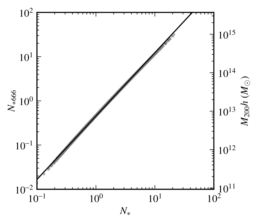
Figure 3.— Richness estimate $N_{*666}$ versus $N_{*}$ for clusters with $N_{*666}>3$ and $\Delta\ln\mathcal{L}\geq 5$ found in the second cluster search iteration. The solid curve is the best-fit power law. On the right axis we show a rough estimate of the cluster mass $M_{200}$, as estimated from $N_{*666}$ in the X-ray stacking analysis of Dai et al. (2007) See Section 2.2.

Our primary richness measurement is $N_{*}$, defined as the number of galaxies brighter than $L_{*}$ within a fixed radius $r<r_{\mathrm{out}}=1.0\,h^{-1}$ Mpc. Though convenient for our purposes, it is not easy to compare to more theoretically motivated indicators, which are usually defined with respect to a virial radius within which the average density is some multiple of the background. To address this issue, we define a second indicator $N_{*666}$ as the number of $L>L_{*}$ galaxies within a virial radius $r_{666}$. We calculate this radius by numerically solving the equation

$$N_{*\Delta_{N}}\equiv N_{*}F(r_{\Delta_{N}}/r_{c})/F(C)=\frac{4\pi}{3}n_{*}\Delta_{N}r_{\Delta_{N}}^{3}\Gamma(1+\alpha,1)$$ (11)

for $r_{\Delta_{N}}$, with the number overdensity $\Delta_{N}$ set to 666, corresponding (for unit bias and $\Omega_{M}=0.3$) to a mass overdensity relative to the critical density $\Delta_{M}=\Delta_{N}\Omega_{M}=200$. The density $n_{*}$ is taken from the field galaxy luminosity function $\phi_{f}$, and $\alpha$ is the slope of the cluster luminosity function $\phi_{c}$. It is worth noting that aside from a relatively unimportant dependence on $\alpha$, $N_{*666}$ is completely determined by $N_{*}$ and $r_{c}$. The two richness indicators are highly correlated, and their values from the second cluster search iteration are plotted against each other in Figure 3. The best-fit relationship between them is $\log N_{*666}=(-0.34\pm 0.01)+(1.43\pm 0.03)\log N_{*}$, and we measure a scatter in $\log(N_{*666})$ of $0.009$ at fixed $N_{*}$. Dai et al. (2007) explore the relationship between $N_{*666}$ and $M_{200}$, the mass of clusters measured within the standard radius $r_{200}$ where the overdensity is 200 times the critical density. They find that they two quantities are nearly linearly related, with

$$\log N_{*666}=$$

$$~{}~{}~{}~{}~{}(1.10\pm 0.04)+(0.87\pm 0.05)\log\left(\frac{M_{200}h_{70}}{10^{14.6}M_{\odot}}\right)~{}.$$ (12)

To give a rough idea of the range of masses of our cluster sample, we show this relationship in Figure 3. The plotted values take into account their use of $h_{70}$, as well as the difference between our second-iteration $N_{*666}$ and that of Dai et al. (2007) due to the change in the cluster luminosity function. We discuss this difference in a few paragraphs.

The number of galaxies actually detected in a cluster of a given richness controls its observability. This is a distance-dependent quantity: for a nearby cluster we detect many faint galaxies that appear brighter than our magnitude limit, while an equally rich distant cluster will manifest only its brightest few galaxies. We define $N_{g666}$ as the number of cluster galaxies within $r<r_{666}$ brighter than the survey magnitude limit:

$$N_{g666}=N_{*666}\frac{\Gamma(1+\alpha,L_{\mathrm{lim}}(z_{c})/L_{*})}{\Gamma(1+\alpha,1)}~{},$$ (13)

where $L_{\mathrm{lim}}(z_{c})$ is the galaxy luminosity corresponding to the survey limit at redshift $z_{c}$. A related quantity appears in the first term in Equation (1). The number of galaxies within the circular sampling radius $R_{\mathrm{samp}}$ brighter than the limiting magnitude is given by

$$A(z)=\frac{g(R_{\mathrm{samp}}/r_{c})}{F(C)}\frac{\Gamma(1+\alpha,L_{\mathrm{lim}}(z)/L_{*})}{\Gamma(1+\alpha,1)}$$ (14)

for a cluster of richness $N_{*}=1$, where $L_{\mathrm{lim}}$ is defined as in Equation (13), and $g(x)$ is defined in Equation (10).

Finally, in some cases we are interested in the probability that a certain galaxy is a cluster member. Despite its similar name, this is not the same as the probability of finding a galaxy near a cluster $P_{c}$. For a galaxy labeled $i$ near a cluster labeled $k$, we define its membership probability as

$$P_{\mathrm{memb}}(i,k)=\frac{P_{c}(i,k)}{\sum_{j}P_{c}(i,j)+P_{f}(i)}~{},$$ (15)

where $P_{f}$ and $P_{c}$ are defined in Equations (2) and (2.1), the and sum is over all clusters. This definition is nearly identical to that of Rozo et al. (2009), except that they consider only the $j=k$ term of the sum.

There is a subtle but important difference between the values of $N_{*}$ and $N_{*666}$ that we find in our first cluster iteration and those we find in the second iteration. This is because we change the parameters of the luminosity function between the iterations, most importantly the cutoff magnitude $M_{K*}$. Since $N_{*}$ is defined as the number of galaxies brighter than $M_{K*}$, we change this count when we change $M_{K*}$. In Section 3.3 we discuss the change in the matched filter luminosity function between the first and second search iterations. As the cluster search algorithm varies $N_{*}$ to maximize the likelihood, it is effectively fitting the matched filter luminosity function to the observed galaxy distribution by varying its normalization. Therefore, our best estimate of the transformation between $N_{*1}$ from the first cluster search iteration and $N_{*2}$ from the second is the ratio of normalizations of the Schechter functions that best fit the stacked cluster luminosity function. We perform these fits in Section 3.3. The normalization of the second-iteration luminosity function is a factor of 0.838 lower than that of the first iteration; therefore, $N_{*2}\approx 0.838N_{*1}$ for any given cluster. With the (reasonable) assumption that $r_{c}$ does not depend on the shape of the luminosity function, the virial richness $N_{*666}$ varies the same way. The transformation of $N_{g666}$ is more complicated; it involves not only the ratio of normalizations but the fraction of galaxies brighter than the survey limit. The ratio of the second-iteration $N_{g666}$ to the first-iteration one is

$$0.838\frac{\Gamma(1+\alpha_{2},L_{\mathrm{lim}}/L_{*2})}{\Gamma(1+\alpha_{1},L_{\mathrm{lim}}/L_{*1})}\frac{\Gamma(1+\alpha_{1},1)}{\Gamma(1+\alpha_{2},1)}~{},$$

where the subscripts 1 and 2 refer to the first and second iterations, and $L_{\mathrm{lim}}$ is the limiting luminosity as in Equation (13). This value is redshift-dependent, varying from 0.868 at $z_{c}=0.01$ to 1.328 at $z_{c}=0.1$. It is unity at a redshift of 0.047, and since this is a fairly typical redshift for our clusters we adopt this value, so that there is no change in $N_{g666}$ between iterations. We tested these ratios by matching a subset of our second-iteration cluster catalog to our first-iteration catalog, and found them to be correct predictions. Throughout this paper, we report the values of $N_{*}$ and $N_{*666}$ calculated by our algorithm without applying the correction factor, but we caution the reader to take care in comparing their values. In some cases we use the factor to define subsets of the cluster catalogs that should be roughly equivalent between iterations, and we note our use of the transformation factors in those instances.

3. Characteristics of Stacked Clusters

We cannot characterize the radial profile, luminosity function, or velocity distribution of individual clusters in any detail, because the typical cluster contains too few galaxies. But by “stacking” large number of clusters, we can determine their average properties. Methods similar to this have been used in several studies (e.g., Carlberg et al., 1996; Dai et al., 2007; Rykoff et al., 2008; Rozo et al., 2010). We apply the process to a sample of clusters with likelihoods $\Delta\ln\mathcal{L}>5$ and expected galaxy number $N_{g666}>3$. K03 found that this last requirement resulted in an extremely pure sample of clusters.

The stacking process consists of selecting the galaxies within some physical radius of the cluster center and constructing a histogram of the relevent quantity (i.e., radial position for a radial profile or absolute magnitude for a luminosity function), subtracting an appropriate background (estimated using the entire galaxy sample), and averaging the results for the sample of clusters. We estimate the uncertainties in our averages using bootstrap resampling, an approach which we advocate for future studies. We resample both the cluster and galaxy lists with replacement to construct the bootstrap uncertainties. In all cases we resample 100 times.

Before stacking, we separate our cluster catalog into richness bins. We divide the space between $N_{*666}=0.1$ and $N_{*666}=30$ into five logarithmic bins 0.5 dex wide. For the first cluster catalog (i.e., the catalog resulting from the first cluster search iteration), this division excludes five clusters with $N_{*666}<0.1$ and two with $N_{*666}>30$, leaving a total of membership of 58, 365, 596, 425, and 85 clusters in the five bins, in increasing order of richness. In the second cluster catalog, we multiply the bin edges by a factor of 0.838 to account for the fact that the richness measurements are systematically lower than they were in the first iteration (see Section 2.2). These five bins contain 46, 450, 867, 594, and 125 clusters. We further subdivide these bins into membership samples with $3\leq N_{g666}<5$, $5\leq N_{g666}<7$, $7\leq N_{g666}<10$, and $N_{g666}\geq 10$ detected galaxies. This is to check whether there is any bias in our estimates of the cluster properties with the number of detected galaxies. Since the number of detected galaxies depends primarily upon redshift, changes between these subsamples could also indicate evolution of average cluster properties, but at the low redshifts of our clusters we expect little evolution.

It is desirable to use a richness estimator with a small scatter relative to the actual cluster richness (e.g., Rozo et al., 2009; Rykoff et al., 2012). Although $N_{*666}$ is useful for comparison with theoretical studies, it is possible that the nature of its definition (i.e., with respect to other noisy quantities) makes it a noisier estimator than the more simply defined $N_{*}$. To check this, we divide the clusters resulting from our second cluster search iteration into bins of $N_{*}$, matching the bin edges to those of our previous bins using the best-fit relation between $N_{*}$ and $N_{*666}$ described in Section 2.2. We examine the uncertainties in our average profiles, velocity distributions, and luminosity functions resulting from the bootstrap resampling, comparing them to those from the $N_{*666}$ binned samples. There are no significant differences in the size of the error bars, so we cannot conclude on those grounds that $N_{*}$ is a better richness estimator than $N_{*666}$. Given the extremely tight correlation between $N_{*}$ and $N_{*666}$, this is not surprising; the richness bins contain nearly identical sets of clusters in both cases.

3.1. Density Profile

We first compare the average surface density distribution $\Sigma(R)$ to the projected NFW we use for the matched filter. We measure the density profiles in a series of logarithmically spaced annuli with inner and outer edges $R_{\mathrm{in},j}<R_{j}<R_{\mathrm{out},j}$, centered on $R_{j}=(R_{\mathrm{in},j}R_{\mathrm{out},j})^{1/2}$, and with area $A_{j}=\pi(R_{\mathrm{out},j}^{2}-R_{\mathrm{in},j}^{2})$. The expected number of background galaxies in an annulus is

$$b_{j} =2\pi B\left[\left(1+R_{\mathrm{in},j}^{2}/D_{A}(z)^{2}\right)^{-1/2}-\left(1+R_{\mathrm{out},j}^{2}/D_{A}(z)^{2}\right)^{-1/2}\right]$$

$$\approx BA_{j}/D_{A}(z)^{2}~{},$$ (16)

where $B$ is the angular surface density of galaxies to the survey magnitude limit (by “background”, we mean a combination of foreground and background galaxies). The higher-order terms in the curved-sky Taylor expansion become important when we examine nearby clusters at large radii. If we count $N_{j}$ galaxies within the $j$-th annulus, the surface density profile of the cluster, scaled by its richness $N_{*}$, is

$$\Sigma(R_{j})=\frac{1}{N_{*}}\frac{N_{*666}}{N_{g666}}\left[\frac{N_{j}-b_{j}}{A_{j}}\right]~{}.$$ (17)

The quantity $(N_{j}-b_{j})/A_{j}$ is the surface number density of cluster galaxies, after subtracting the mean background $b_{j}$. The factor $N_{*666}/N_{g666}$ converts the observed number of galaxies (brighter than the survey magnitude limit) to the average number of $L>L_{*}$ galaxies; see Equation (13). We average this estimate of the surface density over all clusters in each richness and membership bin. At small and medium scales, all the clusters in the sample contribute, but at the largest scales the number of contributing clusters declines slightly because a few clusters overlap the Galactic latitude boundary $|b|>6.0^{\circ}$. We also calculate the average $N_{*}$ and $r_{c}$ for the clusters in each richness bin.

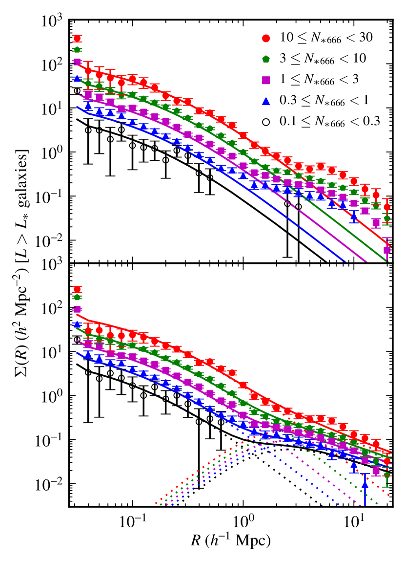
Figure 4.— The projected distributions of galaxies for clusters from the first (top panel) and second (bottom panel) cluster search iterations. They are divided into richness classes from low (open circles) to high (filled circles) richness; note that the second iteration bin edges are smaller than those of the first iteration (see Section 2.2). This figure uses the full sample of clusters with $N_{g666}>3$ (i.e., the union of the membership classes). The points are the observed distributions, with their bootstrap uncertainties. The central density spike is an artifact resulting from our practice of centering every cluster on a galaxy. The first panel shows the projected NFW model. In the second panel, the NFW and two-halo profiles are shown in dotted lines, while their sum is the solid line. Only the NFW component was used in the matched filter, which extends to $1.0\,h^{-1}$ Mpc. Note that we can measure the cluster profile out to 20 Mpc from the center of all but the poorest clusters. The mean background of unrelated galaxies has been subtracted.

Figure 4 shows the projected density profiles of the stacked clusters from the first and second cluster search iterations for each richness bin, including all clusters with at least $N_{g666}\geq 3$ member galaxies and $\Delta\ln\mathcal{L}\geq 5$. In each bin, the profile has been multiplied by the average $N_{*}$ of the bin. We superpose the projected NFW profile $\Sigma(R)$ that was used to find the clusters, calculated using the average $N_{*}$ and $r_{c}$ in each bin. In the second panel we also show an ad-hoc profile for the two-halo contribution suggested by the observed average profiles (more on that in a few paragraphs). It is important to note that the model profiles are not fits to the galaxy profiles, but are simply the matched filter model calculated using the average cluster properties. We note three distinct radial regimes in the profiles.

First, at small radii ($R\lesssim 0.1\,h^{-1}$ Mpc) the profiles are sensitive to the method used to center the clusters. The difficulty of determining the central galaxy density profile of clusters due to the method used to center the cluster is well known (e.g., Beers & Tonry, 1986). The most obvious sign we see is a distinct density spike in the innermost bin; this is due to our practice of always centering a cluster on a galaxy. We avoid “smearing” the contribution of the central galaxy over the region with $R<r_{c}$, but there will always be problems reconstructing a possibly singular average central density profile in the presence of the shot noise from the galaxies sampling the profile. We experimented with using a cluster position estimated by averaging the membership probability weighted positions of the cluster galaxies. While this eliminated the central spike, the profile shape began to depend on the number of member galaxies $N_{g666}$. Essentially, we measure the true average profile convolved with the position measurement errors, and these increase considerably as the number of member galaxies available for the average decreases. This problem has been seen by Dai et al. (2007) and Rykoff et al. (2008), who both stack X-ray images of optically-selection clusters. Despite these problems, our profiles match the expected shape reasonably well apart from the innermost radial bin.

Second, on intermediate scales ($0.1\,h^{-1}$ Mpc $\lesssim R\lesssim 1.6\,h^{-1}$ Mpc), which dominate our detection and parameter estimation, the average surface density of the galaxies matches reasonbly well the profile shape expected from our matched filter. The observed and NFW surface density profiles have formal chi-square differences, for 13 degrees of freedom, of 9.0 to 46 for the first iteration and 2.8 to 42 for the second iteration. These large values arise largely from $\sim 10\%$ normalization differences between the data and the model (which was calculated with no free parameters); these differences are unimportant for the matched filter, where the normalization is free to vary.

Third, on large scales ($R\gtrsim 1.6\,h^{-1}$ Mpc), the observed surface density lies above the projected NFW profile. The NFW model represents only the virialized regions of the cluster and neglects the correlated structure outside the virial radius — the “two-halo” term, in the parlance of the halo model of large scale structure (e.g., Cooray & Sheth, 2002). This outer region of clusters should provide a good testing ground for the halo model because it represents the dividing line between linear and nonlinear regimes. We create a crude model for the profile of the two-halo term consisting of a broken power law:

$$\Sigma_{\mathrm{2h}}(R)=\frac{a_{\mathrm{2h}}(N_{*})\left(R/R_{\mathrm{2h}}\right)^{\beta_{\mathrm{in}}}}{\left(1+R^{2}/R_{\mathrm{2h}}^{2}\right)^{(\beta_{\mathrm{in}}+\beta_{\mathrm{out}})/2}}~{},$$ (18)

where $a_{\mathrm{2h}}(N_{*})$ is a richness-dependent normalization constant for the two-halo term and $R_{\mathrm{2h}}$ is a break radius. The inner and outer slopes $\beta_{\mathrm{in}}$ and $\beta_{\mathrm{out}}$ we set to 2 and 0.8 respectively; the former because it made the enclosed mass an analytic function, and the latter by analogy with the slope of typical correlation functions on these scales. We adjust the normalization and scale radius until they roughly match the observed second-iteration profile, finding that $a_{\mathrm{2h}}(N_{*})=(0.17\pm 0.01)N_{*}^{(0.33\pm 0.04)}\,h^{2}\,\mathrm{Mpc}^{-2}$ and that $R_{\mathrm{2h}}=(1.66\pm 0.10)\,h^{-1}$ Mpc. We do not add the two-halo term to the matched filter in the second cluster search iteration, because its contribution inside $1.0\,h^{-1}$ Mpc (the sampling radius) is very small relative to the NFW component.

For second-iteration clusters, we repeat the stacking process for the membership subsamples of each richness bin in order to check for evolution of the cluster profiles with the number of detected galaxies. The resulting richness estimates are shown in Figure 5. We plot only samples where the product of the number of clusters and the average value of $N_{g666}$ is greater than 30; this excludes three low-richness samples. On scales less than $\sim 1\,h^{-1}$ Mpc, we do not see any evidence for changes in the profile with the number of visible galaxies, unless the profile is very noisy.

3.2. Velocity Distribution

Our cluster search algorithm produces two estimates of the velocity dispersion of each cluster. The first estimate is the value of $\sigma_{c}$ used in the matched filter. We maximize the likelihood for each cluster by varying the velocity dispersion using MCMC optimization, subject to our priors. We also compute the velocity dispersion using galaxies with redshift measurements within $Cr_{c}$ of the center of each cluster, weighting the contribution of each galaxy by its cluster membership probability $P_{\mathrm{memb}}$ (see Equation (15)). We average the latter velocity dispersion estimate in each richness bin, and use this average to define our model in the following analysis.

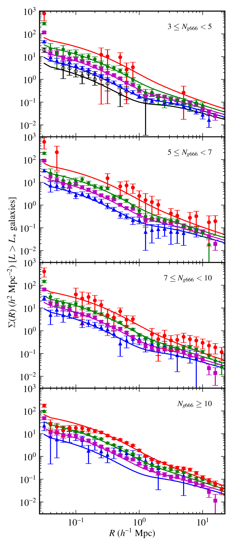
Figure 5.— Projected cluster profiles for cluster subsamples with different numbers of detectable galaxies $N_{g666}$. The clusters with the fewest visible galaxies are in the top panel, and the number increases toward the bottom panel. The points’ colors and shapes indicate richness bin, as in Figure 4, and the solid curves show the sum of the NFW and two-halo term. We do not see strong evidence for evolution in the profile with $N_{g666}$.

As with the cluster density profiles, the typical cluster contains too few galaxies to accurately estimate the velocity distribution in a non-parametric way. So we again stack large numbers of clusters in fixed richness bins to determine the average velocity distribution. We first identify all galaxies with measured redshifts within the projected virial radius, $R\leq r_{666}$, of each cluster, so as to compare velocity histograms inside the virialized region for clusters of differing richness. We discard those galaxies which lack redshift measurements; this should be relatively unbiased with respect to the velocity distribution since any target selection method for measuring redshifts is unbiased with respect to the relevant velocity differences. We then construct histograms of the rest frame line of sight velocities (relative to the systemic velocity) $\Delta v=(v-cz_{c})/(1+z_{c})$, considering only velocities where $|\Delta v|\leq 2000$ km s^-1. We use variable bin widths of 50, 75, 100, 150, and 250 km s^-1 for the five richness bins. Finally, we average the histograms over the clusters in each richness bin, excluding clusters with $N_{v}<5$ galaxies with measured redshifts and clusters with virial radii extending into the region where $|b|<6^{\circ}$. The requirement of five redshift measurements limits the effect of the sample variance bias. We also calculate the average richness and velocity dispersion of the clusters in each richness bin, weighted by $N_{v}-1$.

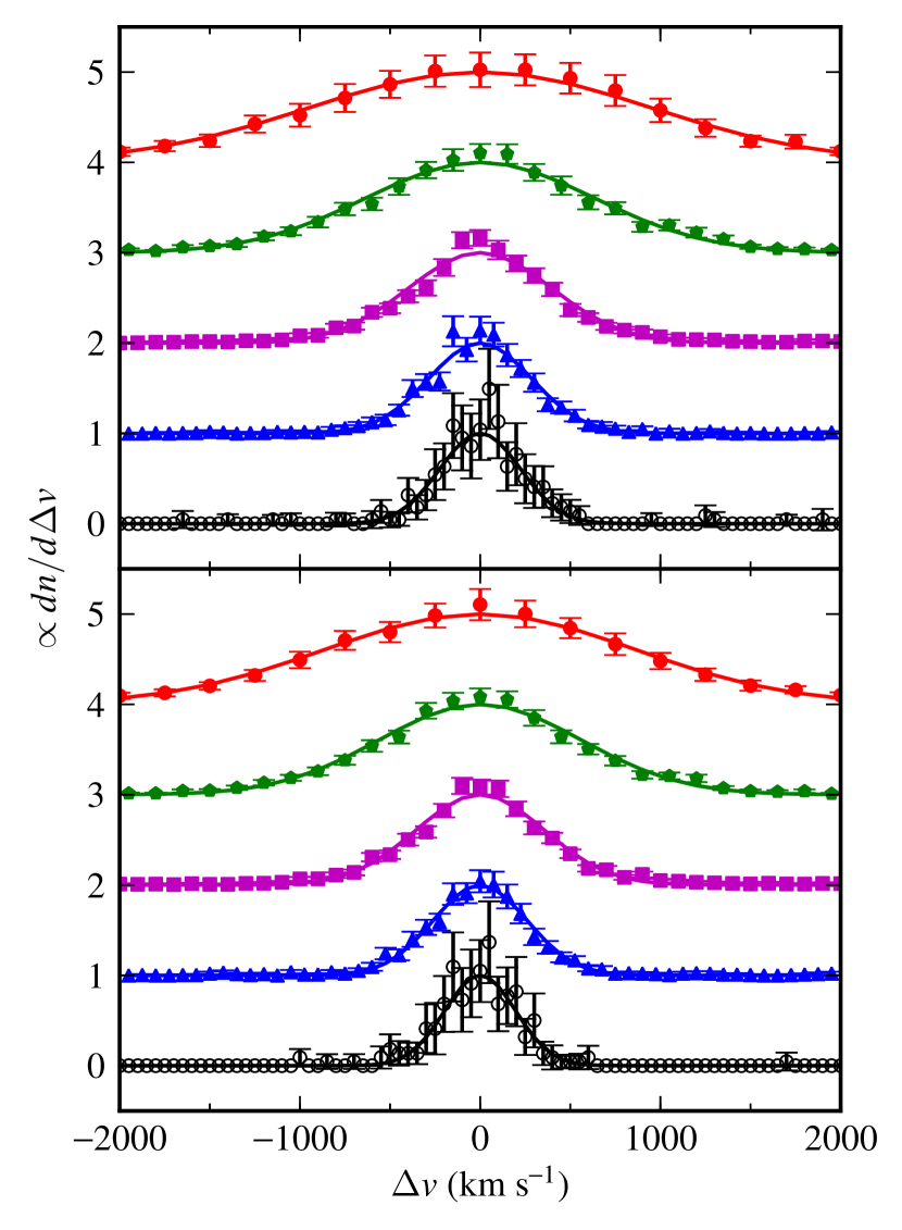
Figure 6.— The rest-frame line of sight velocity distribution of the first-iteration (first panel) and second-iteration (second panel) cluster galaxies in the five richness bins. The points show the average velocity distributions, with the same colors and shapes as in Figure 4, and the solid curves are the Gaussian models used by the matched filter.

Figure 6 shows the velocity distributions measured in this way for the first and second cluster search iterations, for the same richness bins we used for our profile measurement. Superposed on the distributions are Gaussian curves with widths set by the average velocity dispersion in the bins. The normalization of the curves is arbitrary, and they are adjusted to match the observed distributions. We find excellent agreement between the predicted curve and the observed distribution. Figure 7 shows the velocity distributions as a function of visible galaxy number $N_{g666}$. We impose the same cut as was previously used to weed out three low-richness samples. No significant evolution of the velocity distributions with the number of detected galaxies $N_{g666}$ can be seen. Although the velocity distributions look somewhat narrow in the lowest-membership sample, we think this is due to the low number of galaxies per cluster.

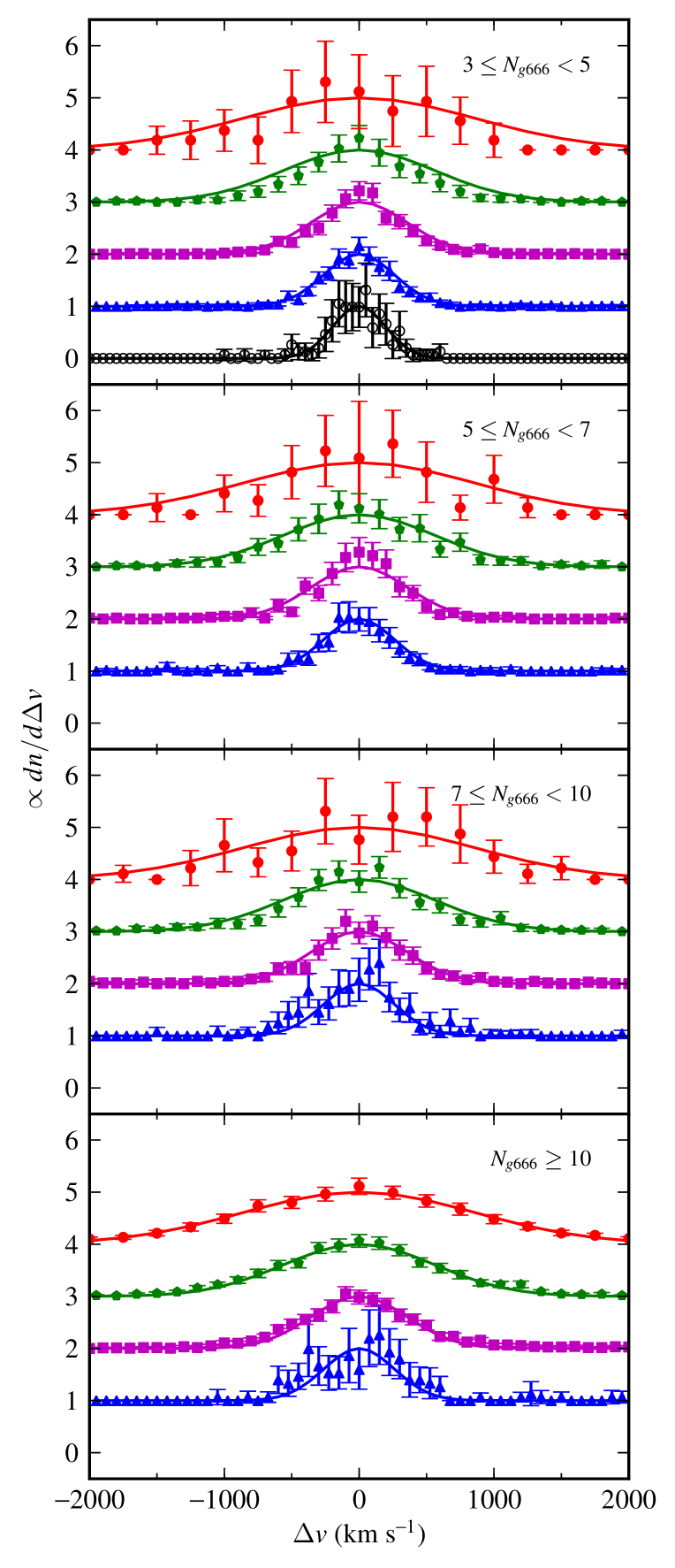
Figure 7.— Velocity distributions for cluster subsamples with different numbers of detectable galaxies $N_{g666}$, which increases from the first frame to the last. The points’ colors and shapes indicate richness bin, as in Figure 6, and the solid curves are identical to those in that figure’s second panel. We see no strong evidence for evolution of the velocity distributions with $N_{g666}$.

One advantage of the stacked clusters is that they contain many galaxies, so it is easy to estimate a Gaussian width without using a statistical method that is dominated by the tails of the distribution. We clip the velocity distributions at twice the average velocity dispersion for each richness bin. We then sort the velocity differences and estimate the velocity dispersion as one-half the velocity range encompassing 68.3% of the galaxies centered on the median. Like a simple velocity dispersion, this estimate is exact for a Gaussian distribution, but it is insensitive to interloping field galaxies. The resulting velocity dispersion estimates are reported, along with the dispersions determined by averaging over each richness bin, in Table 1. The differences between the two estimates are less than 10%.

Table 1Velocity Dispersions

Richness	$\langle\sigma_{c}\rangle$ (km s-1)	$\sigma_{\mathrm{sort}}$ (km s-1)
$0.1\leq N_{*666}<0.3$	$197$	$190$
$0.3\leq N_{*666}<1$	$261$	$250$
$\phantom{0}\phantom{.}1\leq N_{*666}<3$	$357$	$338$
$\phantom{0}\phantom{.}3\leq N_{*666}<10$	$561$	$531$
$\phantom{.}10\leq N_{*666}<30$	$862$	$821$

3.3. Luminosity Function

The final distribution we consider is the luminosity function of the cluster galaxies. Since clusters at different distances have different galaxy luminosities corresponding to the survey magnitude limit, some care is required in combining clusters within a richness bin. We first construct a histogram of the absolute magnitudes of galaxies within $R_{\mathrm{samp}}=1.0\,h^{-1}$ Mpc of each cluster center, with bins $1/3$ mag in width. Each histogram extends to the faintest bin whose faint edge is brighter than the survey limit. In this same set of magnitude bins we calculate the “background” of interloping galaxies by taking the distribution of apparent magnitudes of our galaxy sample, shifting this distribution by the distance modulus $\mathcal{D}(z_{c})$, and scaling the resulting distribution by the ratio of the angular area of the cluster to that of the whole survey. We subtract this background from the luminosity function and scale the difference by the factor $N_{*}g(R_{\mathrm{samp}}/r_{c})/F(C)$ to account for our cylindrical sampling volume. Finally, we average the result over all the clusters in each richness bin, weighting the clusters by this same factor. The number of clusters contributing to the luminosity function estimate is a strong function of absolute magnitude; the faintest bins only have contributions from the nearest clusters, while the brightest bins average over tens to hundreds of clusters, depending on the richness and membership bin. As before, we exclude clusters with sampling radii extending into the excluded region of low Galactic latitude where $|b|<6^{\circ}$.

Figure 8 shows the observed cluster galaxy luminosity function for clusters from our first and second search iterations. In each case, the luminosity function used for the matched filter is plotted as a short-dashed curve, with a normalization adjusted to best fit the observed data. The curve in the first panel clearly lies below the data, especially at the bright end. So we fit a second Schechter function to the data; this is plotted as a dotted curve. This function was characterized by $M_{K*}=-23.59\pm 0.05$ mags and $\alpha=-1.08\pm 0.03$. We used this function for the second matched filter; it is therefore the short-dashed curve in the second panel. It closely matches the best-fit Schechter function for that panel, which has parameters $M_{K*}=-23.64\pm 0.05$ mags and $\alpha=-1.07\pm 0.03$. This fit is good, producing a chi-square of 169.6 for 130 degrees of freedom.

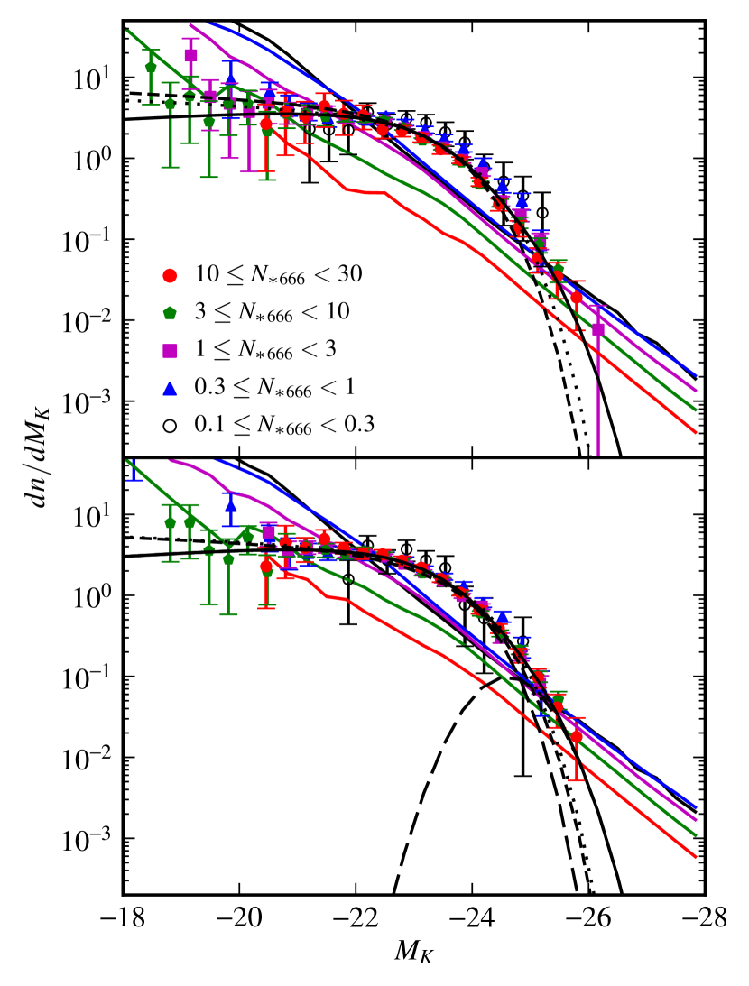
Figure 8.— The cluster luminosity function for first-iteration (first panel) and second-iteration (second panel) clusters in the five richness bins. The points show the measured luminosity functions, normalized to unit $N_{*}$. In each panel, the short-dashed curve signifies the Schechter function used in the matched filter, and the dotted curve is the best-fit Schechter function. The solid curves indicate the best-fit sum of Schechter and BCG components, which are also shown separately as long-dashed lines in the second panel. The slanted lines show the level of foreground/background contamination that is subtracted to make the estimate of the luminosity function for each richness class; the contrast of clusters relative to this contamination depends strongly on richness. At very high and very low luminosities, the foreground/background subtraction fails.

There has been considerable interest in the luminosity fuction of BCGs and whether they lie on the same Schechter function as satellite galaxies (e.g., Yang et al., 2008). In Figure 8 we see a small excess at the bright end of the luminosity function relative to the best-fit (dotted) Schechter function, suggesting that we are seeing a separate population of BCGs. We parameterize this population using a Gaussian luminosity distribution in magnitude space. To investigate the BCG population, we attempt to identify in each cluster the galaxy with the greatest probability of being the BCG. The BCG probability is the product of the galaxy’s cluster membership probability, defined in Equation (15), and the probability that the galaxy’s luminosity is drawn from the Gaussian BCG distribution. For the clusters found in the first iteration, we made a guess at this distribution, centering the Gaussian at $-25.1$ mags, with a variance of $(0.4~{}\mathrm{mags})^{2}$. The exact parameters of this distribution are not very important; its main function is to help us rank the galaxies by BCG probability. We exclude any galaxy that lacks a redshift measurement, has membership probability $P_{\mathrm{memb}}<0.5$, or is farther than $R_{\mathrm{samp}}=1.0\,h^{-1}$ Mpc from the cluster center. Out of our sample of 1532 clusters with $N_{g666}>3$, this process yields BCGs for 1507. The magnitude distribution of these galaxies is close to Gaussian in shape, and has mean $-24.61$ mags and variance $(0.56~{}\mathrm{mags})^{2}$. We adopt these parameters for the BCG luminosity distribution, and repeat our fit of the luminosity function with this Gaussian term included. We find best fit values of $M_{K*}=-23.22\pm 0.07$ and $\alpha=-0.90\pm 0.05$, with the BCG distribution peaking at $(0.045\pm 0.003)\phi_{c}(M_{K*})$. This two-part luminosity function is shown as a solid curve in the first panel of Figure 8. The best-fit luminosity function for the second-iteration cluster sample is nearly identical, with $M_{K*}=-23.27\pm 0.07$ mags and $\alpha=-0.89\pm 0.05$. The BCG curve is centered on $-24.57$ mags, with a variance of $(0.59~{}\mathrm{mags})^{2}$, and reaches a maximum of $(0.048\pm 0.009)\phi_{c}(M_{K*})$. This function is likewise plotted as a solid curve in the second panel of Figure 8, and its components are shown as long-dashed curves. This fit is slightly better than the Schechter-only fit, with a chi-square of 141.6 for 129 degrees of freedom.

The luminosity function calculated using the membership subsamples is shown in Figure 9. In each panel we also plot a solid curve showing the same best-fit luminosity function as is shown in the second panel of Figure 8. We again see no strong evidence of evolution with the number of observed cluster members.

Our luminosity function results broadly agree with previous estimates for the IR luminosity functions of cluster galaxies. For example, Balogh et al. (2001) estimate the $K$-band luminosity function using 2MASS galaxies matched to groups and clusters in the LCRS. For groups ($\sigma<400$ km/s, or $N_{*666}\lesssim 3$), they find estimates of $M_{K*}=-23.58\pm 0.13$ and $\alpha=-1.14\pm 0.26$, whereas for clusters ($\sigma>400$ km/s, or $N_{*666}\gtrsim 3$) they find $M_{K*}=-23.81\pm 0.40$ and $\alpha=-1.30\pm 0.43$. Similarly, Lin et al. (2004) examine X-ray selected clusters in 2MASS data, finding $-1.1\lesssim\alpha\lesssim-0.84$ and $-24.57\leq M_{K*}\leq-23.25$. In their study of clusters from the Canadian Network for Observational Cosmology survey (Yee et al., 1996) at a median redshift of $z=0.3$, Muzzin et al. (2007) find $M_{K*}=-23.76\pm 0.15$ and $\alpha=-0.84\pm 0.08$. We have adjusted the values of $M_{K*}$ from Lin et al. (2004) and Muzzin et al. (2007) to account for their use of $h=0.7$.

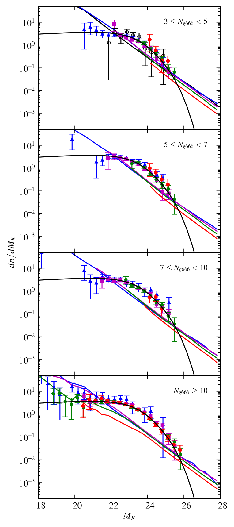
Figure 9.— Cluster luminosity function for cluster subsamples with different numbers of detectable galaxies $N_{g666}$, which increases from the first frame to the last. The points’ colors and shapes indicate richness bin, as in Figure 8, and the solid curves are identical to those in that figure’s second panel. We see no strong evidence for evolution of the luminosity function with $N_{g666}$.

4. Priors

As alluded to in previous sections, we make a number of adjustments to the likelihood function in Equation (1) in order to stabilize parameter estimation and reflect prior knowledge. Each modification takes the form of an additive term, usually the logarithm of a multiplicative prior probability distribution. The exact formulas for these additions, labeled Prior I through Prior VI, are listed in Table 2, with their parameters listed in Table 3. The first prior imposes a prior on the richness $N_{*}$ with a slope of $-2$, and turning over at $N_{*}=0.1$, the expected richness of the poorest groups. This enforces a reasonable mass function for clusters, with a power-law slope. Prior II makes the likelihood independent of $\sigma_{c}$ when the candidate cluster contains only one galaxy with a redshift measurement, removing a bias in the optimization of this parameter’s value. Prior III reflects empirical relationships between $N_{*}$ and the parameters $\sigma_{c}$ and $r_{c}$, imposing a Gaussian centered on a power-law relationship between the richness and the parameter, with a width designed to match the scatter in the parameter at fixed richness. In using these priors, we are following K03 (although they do not include the prior on the $N_{*}-r_{c}$ relationship, because unlike us they fix $r_{c}=0.2\,h^{-1}$ Mpc for all clusters). We also include three priors not used by K03, labeled Priors IV through VI. The first of these is very similar to Prior I; it requires clusters with large velocity dispersions and core radii to be rare, taking the power-law slope of the mass function and of the mass-observable relation as parameters. Prior V imposes a Fermi function cutoff on the parameters $\sigma_{c}$ and $r_{c}$, ruling out very small values. Finally, Prior VI puts a Gaussian prior on the difference between the line of sight velocity of the central galaxy and that of the cluster, and specifies that the central galaxy ought to be around $L_{*}$ or brighter.

Table 2Priors

Label	Formula	Comments
Prior I	$-\ln[1+(N_{*}/N_{*}^{I})^{2}]$	Cluster mass function
Prior II	$+\ln(\sigma_{c}/\sigma_{c}^{II})$	Unbiased estimate of $\sigma_{c}$
Prior III	$-1/2\left[\log(\sigma_{c}/\sigma_{c}^{III})-a^{III}_{0}\log(N_{*})\right]^{2}/(a^{III}_{1})^{2}$	Empirical $N_{*}-\sigma_{c}$ correlation
	$-1/2\left[\log(r_{c}/r^{III}_{c})-a^{III}_{2}\log(N_{*})\right]^{2}/(a^{III}_{3})^{2}$	Empirical $N_{*}-r_{c}$ correlation
Prior IV	$+[\alpha_{\sigma}(1-\gamma)-1]\ln(\sigma_{c}/\sigma_{c}^{IV})$	Mass function and $M_{cl}-\sigma_{c}$ relation
	$+[\alpha_{r}(1-\gamma)-1]\ln(r_{c}/r^{IV}_{c})$	Mass function and $M_{cl}-r_{c}$ relation
Prior V	$-\ln(1+\exp[(\sigma_{c}^{V}-\sigma_{c})/\Delta\sigma_{c}^{V}])$	Fermi function enforcing $\sigma_{c}\gtrsim\sigma_{c}^{V}$
	$-\ln(1+\exp[(r^{V}_{c}-r_{c})/\Delta r^{V}_{c}])$	Fermi function enforcing $r_{c}\gtrsim r^{V}_{c}$
Prior VI	$-1/2(v_{pec}/v^{VI}_{pec})^{2}$	Peculiar velocity of central galaxy
	$-2.5a^{VI}\log(1+L_{*}/L_{cen})$	Brightness of central galaxy

Table 3Prior parameter values

Label	Parameter	Iter. 1 Value	Iter. 2 Value
Prior I	$N_{*}^{I}$	$0.1$	$0.1$
Prior II	$\sigma_{c}^{II}$	$1000~{}\mathrm{km}~{}\mathrm{s}^{-1}$	$1000~{}\mathrm{km}~{}\mathrm{s}^{-1}$
Prior III	$a^{III}_{0}$	$0.526$	$0.445$
	$a^{III}_{1}$	$0.0744$	$0.153$
	$a^{III}_{2}$	$0.114$	$0.155$
	$a^{III}_{3}$	$0.071$	$0.037$
	$\sigma_{c}^{III}$	$254~{}\mathrm{km}~{}\mathrm{s}^{-1}$	$250~{}\mathrm{km}~{}\mathrm{s}^{-1}$
	$r^{III}_{c}$	$0.231~{}\mathrm{Mpc}$	$0.203~{}\mathrm{Mpc}$
Prior IV	$\gamma$	$1.8$	$1.8$
	$\alpha_{\sigma}$	$2.0$	$2.0$
	$\alpha_{r}$	$2.25$	$2.25$
	$\sigma_{c}^{IV}$	$800~{}\mathrm{km}~{}\mathrm{s}^{-1}$	$800~{}\mathrm{km}~{}\mathrm{s}^{-1}$
	$r^{IV}_{c}$	$0.2~{}\mathrm{Mpc}$	$0.2~{}\mathrm{Mpc}$
Prior V	$\sigma_{c}^{V}$	$200~{}\mathrm{km}~{}\mathrm{s}^{-1}$	$200~{}\mathrm{km}~{}\mathrm{s}^{-1}$
	$\Delta\sigma_{c}^{V}$	$10~{}\mathrm{km}~{}\mathrm{s}^{-1}$	$10~{}\mathrm{km}~{}\mathrm{s}^{-1}$
	$r^{V}_{c}$	$0.1~{}\mathrm{Mpc}$	$0.1~{}\mathrm{Mpc}$
	$\Delta r^{V}_{c}$	$0.01~{}\mathrm{Mpc}$	$0.01~{}\mathrm{Mpc}$
Prior VI	$v^{VI}_{pec}$	$200~{}\mathrm{km}~{}\mathrm{s}^{-1}$	$200~{}\mathrm{km}~{}\mathrm{s}^{-1}$
	$a^{VI}$	$1.0$	$1.0$

Some of the prior parameters listed in Table 3 are simply constant offsets to the likelihood, and are thus unimportant except insofar as they may admit or exclude clusters with likelihoods near the cutoff value. The parameters $\sigma_{c}^{II}$, $\sigma_{c}^{IV}$, and $r_{c}^{IV}$ fall in this category. We set them to nominal values, adopting K03’s value for $\sigma_{c}^{II}$. For Priors I and III, we use the same parameter values as K03 for the first cluster search iteration, making a guess for the values for the relationship between $N_{*}$ and $r_{c}$. For Priors IV and V we use theoretically motivated guesses at the parameter values. In particular, Prior IV encodes the expectation that $dN/dM\propto M^{-\gamma}$ and that $M\propto\sigma_{c}^{\alpha_{\sigma}}\propto r_{c}^{\alpha_{r}}$. Tinker et al. (2008) parameterize the cluster mass function using a more complicated functional form, but we can approximate it as a power law of slope $\gamma=-1.8$.

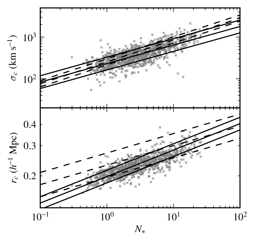
Figure 10.— Velocity dispersion $\sigma_{c}$ (first panel) and core radius $r_{c}$ (second panel) versus richness $N_{*}$, for selections of clusters from the first cluster search iteration. The dashed lines indicate the relationship used in Prior III during the first search iteration, with its $1\sigma$ width, and the solid lines indicate the relationship and width used during the second iteration. See Section 4, as well as Tables 2 and 3.

Our third prior reflects empirical relationships between cluster richness and other properties. We examine the correlations between these properties in subsets of the clusters found in our first cluster search iteration, in order to update the parameters of this prior for the second iteration. We turn first to the $N_{*}-\sigma_{c}$ correlation. For this test we used a subset of 902 clusters with likelihoods $\Delta\ln\mathcal{L}>20$, expected number of visible galaxies $N_{g666}>3$, and measured velocity dispersions (i.e., we excluded clusters with too few redshift measurements). The top panel of Figure 10 shows the distribution of these clusters. We find a strong correlation, with a Pearson coefficient $r=0.75$. The prior used in the first iteration is plotted with its $1\sigma$ contours, and matches the observed distribution well. We also plot a fit to the data, with lines indicating the scatter about the fit. The best-fit relationship is $\log(\sigma_{c})=(2.36\pm 0.05)+(0.445\pm 0.088)\log(N_{*})$, with a scatter of $0.153$ dex. The updated parameters for Prior III that result from this fit are listed in Table 3. Because the meaning of $N_{*}$ changes between iterations, we use the transformation factor calculated in Section 2.2 to express the empirical relationships in terms of the second-iteration richness. This simply results in a slightly different offset to the relation; these offsets are reflected in the values of $\sigma_{c}^{III}$ and $r_{c}^{III}$ reported in Table 3. When we examine the same relationship after the second cluster finding iteration, the best-fit relationship and the scatter are essentially unchanged.

We examine next the correlation between $N_{*}$ and $r_{c}$, using the same subsample of clusters as before but also including 27 clusters with unmeasured velocity dispersions. As seen in the bottom panel of Figure 10, there is again a strong correlation (Pearson $r=0.77$). We plot the prior used in the first cluster-finding iteration. The observed correlation is offset from the prior relation, and has a scatter smaller than the width of the prior. We find that if we adjust the prior in the second search iteration to match this empirical relationship, a similar offset and further reduced scatter are apparent in the second-iteration clusters. This indicates that the galaxy distribution is not constraining $r_{c}$ for individual clusters, but that it is being determined predominantly by the priors (particularly by the combination of Prior III and Prior IV, which favors smaller values of $r_{c}$). This is not particularly surprising, since the detailed radial density profile of a single cluster cannot be well constrained unless a great many member galaxies are detected. Therefore we abandon the strategy of determining the parameters of Prior III using individual $r_{c}$ values and turn to the stacked profiles described in Section 3.1 and shown in the first panel of Figure 4. We fit the projected NFW profile from Equation 10 to the stacked profiles in each of the five richness bins, varying the normalization and the scale radius $r_{c}$. We restrict our fits to radii smaller than $1\,h^{-1}$ Mpc, and ignore the innermost radial bin, which is biased high because of the central galaxy in each cluster. We use the resulting values and uncertainties in $r_{c}$ to perform a power-law fit for the relationship between $\langle N_{*}\rangle$ (the average $N_{*}$ in each richness bin) and $r_{c}$. We obtain a logarithmic slope of $0.155\pm 0.068$ and normalization (i.e., $r_{c}$ for $N_{*}=3$) of $0.235\pm 0.012$. Since this relationship is determined using the stacked profiles of actual clusters, it is not directly affected by Prior III; nevertheless, it does not differ wildly from the first-iteration relationship. In our second cluster search iteration, we update the parameters of Prior III to these best-fit values (see Table 3). We set the width of the prior $a_{3}^{III}$ to three times the uncertainty in the normalization, to account for the additional uncertainty in the slope.

5. Conclusions

We follow up on the search for galaxy clusters in the 2MASS catalog described by K03, using an iterative process to check and adjust several of the adjustable aspects of the algorthm. The most important component of the search process is the matched filter itself, that is the description of the characteristics of clusters. We check the projected density profile shape and velocity distribution of clusters, and the luminosity function of their galaxies by stacking clusters in bins of richness. Overall, we find that the cluster model used by K03 is mostly accurate, with radial profiles closely matching the projected NFW model at radii less than $1\,h^{-1}$ Mpc and velocity distributions matching the expected Gaussian distributions very well. At large radii, out to $\sim 20\,h^{-1}$ Mpc, the observed density profile lies above the projected NFW profile. We attribute the excess density to correlated structure and construct a toy profile to fit this “two-halo” term, but because our matched filter only searches for galaxies within $1\,h^{-1}$ Mpc we do not bother to add it to our matched filter. The main discrepancy between the stacked clusters and the matched filter that was used to find them is in the luminosity function, which we find to underestimate the fraction of bright galaxies. After updating the matched filter with the best-fit Schechter function, we find that the second-iteration clusters match the filter well. The best-fit function has $M_{K*}=-23.64\pm 0.04$ and $\alpha=-1.07\pm 0.03$. Though a single Schechter function fits the data reasonably well, we find a slightly better fit when we add a Gaussian component at the bright end, suggesting that a separate population of BCGs is present. Based on our best guess of the BCGs in a subset of our clusters, we estimate that the Gaussian is centered at a $K$ magnitude of $-24.57$, with a variance of ($0.59$ mag)². Including this component causes the Schechter parameters to change considerably; their new best-fit values are $M_{K*}=-23.27\pm 0.07$ and $\alpha=-0.89\pm 0.05$. The Gaussian BCG component peaks at a value of $(0.048\pm 0.009)\phi(M_{K*})$. We do not find that the average profiles, velocity distributions, or luminosity functions of clusters varied with $N_{g666}$, the (distance-dependent) number of cluster galaxies that we expect to be brighter than the survey limit.

We also update the priors that are added to the likelihood function. We include the three priors used by K03, including one (labeled Prior III) which takes into account the empirical relationship between richness and velocity dispersion and adding one for the analogous relationship between richness and core radius. We also add three more priors in an effort to improve the completeness and purity characteristics of the cluster sample. The first of these, which we label Prior IV, discourages clusters with large velocity dispersions and core radii, as they are associated with (rare) massive clusters. Another puts lower limits on the values that these variables can take, and the last puts a prior on the central galaxies of clusters, encouraging them to be brighter than $L_{*}$ and to have small peculiar velocities. We use the clusters found in our first cluster search iteration to tune the empirical relationships on which Prior III is based for the second iteration.

After adjusting the parameters of the matched filter and the priors, we repeat our search for clusters. The richness and redshift distributions of the resulting sample of 7624 cluster candidates with $\Delta\ln\mathcal{L}\geq 5$ (2087 with $N_{g666}>3$) are shown in Figure 2. This is a larger sample than the 5793 (1532 with $N_{g666}>3$) found in the first iteration. When we repeat the stacking analysis on this second catalog, we find that the shape of the filter is well-matched to the average properties of the clusters. We further subdivide the clusters into membership samples with different values of $N_{g666}$ in order to test for evolution in the cluster parameters with the number of detected cluster galaxies, and find no strong evidence for such evolution.

We mention in closing two technical points. First, we have introduced the general approach for studying clusters of “catalog bootstrap resampling”. By simultaneously resampling both the cluster catalog and the galaxies, we can include many statistical uncertainties in a well-defined manner. This bootstrap approach could also be applied to the galaxy catalog during the process of finding clusters, where the variance in the resulting cluster catalogs and properties would probe many, though not all, of the systematic problems associated with identifying clusters, and would yield meaningful constraints on the purity of the catalog. The one operational issue is that repeated galaxies should be spatially shifted away from one another in order to avoid overly artificial density spikes, but not by so much that density profiles are overly smoothed. This suggests scales of order $r_{c}$, but tests in artificial catalogs can be used to test and optimize this scheme. Second, while in this work we have stacked clusters in order to “manually” adapt the matched filter used to find clusters, the process could in principle be automated. For instance, once an initial catalog is found, one could adjust the parameters of the matched filter to maximize the overall likelihood value based on the fixed properties of that cluster catalog. A new catalog could then be constructed using that updated matched filter. Note that this is still an iterative process; it is doubtful that an attempt to simultaneously find clusters and optimize the matched filter would be numerically stable.

References

- Abazajian et al. (2005) Abazajian, K., et al. 2005, AJ, 129, 1755
- Abell (1958) Abell, G. O. 1958, ApJS, 3, 211
- Abell et al. (1989) Abell, G. O., Corwin, Jr., H. G., & Olowin, R. P. 1989, ApJS, 70, 1
- Allen et al. (2008) Allen, S. W., Rapetti, D. A., Schmidt, R. W., Ebeling, H., Morris, R. G., & Fabian, A. C. 2008, MNRAS, 383, 879
- Bahcall (1988) Bahcall, N. A. 1988, ARA&A, 26, 631
- Balogh et al. (2001) Balogh, M. L., Christlein, D., Zabludoff, A. I., & Zaritsky, D. 2001, ApJ, 557, 117
- Bartelmann (1996) Bartelmann, M. 1996, A&A, 313, 697
- Beers & Tonry (1986) Beers, T. C., & Tonry, J. L. 1986, ApJ, 300, 557
- Böhringer et al. (2001) Böhringer, H., et al. 2001, A&A, 369, 826
- Bottinelli et al. (1990) Bottinelli, L., Gouguenheim, L., Fouque, P., & Paturel, G. 1990, A&AS, 82, 391
- Carlberg et al. (1996) Carlberg, R. G., Yee, H. K. C., Ellingson, E., Abraham, R., Gravel, P., Morris, S., & Pritchet, C. J. 1996, ApJ, 462, 32
- Carlstrom et al. (2000) Carlstrom, J. E., Joy, M. K., Grego, L., Holder, G. P., Holzapfel, W. L., Mohr, J. J., Patel, S., & Reese, E. D. 2000, Physica Scripta Volume T, 85, 148
- Colless et al. (2001) Colless, M., et al. 2001, MNRAS, 328, 1039
- Cooray & Sheth (2002) Cooray, A., & Sheth, R. 2002, Phys. Rep., 372, 1
- Crook et al. (2007) Crook, A. C., Huchra, J. P., Martimbeau, N., Masters, K. L., Jarrett, T., & Macri, L. M. 2007, ApJ, 655, 790
- da Costa et al. (1998) da Costa, L. N., et al. 1998, AJ, 116, 1
- Dai et al. (2007) Dai, X., Kochanek, C. S., & Morgan, N. D. 2007, ApJ, 658, 917
- Dong et al. (2008) Dong, F., Pierpaoli, E., Gunn, J. E., & Wechsler, R. H. 2008, ApJ, 676, 868
- Dressler & Gunn (1992) Dressler, A., & Gunn, J. E. 1992, ApJS, 78, 1
- Ebeling et al. (1998) Ebeling, H., Edge, A. C., Bohringer, H., Allen, S. W., Crawford, C. S., Fabian, A. C., Voges, W., & Huchra, J. P. 1998, MNRAS, 301, 881
- Einasto et al. (2001) Einasto, M., Einasto, J., Tago, E., Müller, V., & Andernach, H. 2001, AJ, 122, 2222
- Falco et al. (1999) Falco, E. E., et al. 1999, PASP, 111, 438
- Gioia et al. (1990) Gioia, I. M., Henry, J. P., Maccacaro, T., Morris, S. L., Stocke, J. T., & Wolter, A. 1990, ApJ, 356, L35
- Gladders & Yee (2000) Gladders, M. D., & Yee, H. K. C. 2000, AJ, 120, 2148
- Goto et al. (2003) Goto, T., Yamauchi, C., Fujita, Y., Okamura, S., Sekiguchi, M., Smail, I., Bernardi, M., & Gomez, P. L. 2003, MNRAS, 346, 601
- Henry (2000) Henry, J. P. 2000, ApJ, 534, 565
- Högbom (1974) Högbom, J. A. 1974, A&AS, 15, 417
- Huchra et al. (1983) Huchra, J., Davis, M., Latham, D., & Tonry, J. 1983, ApJS, 52, 89
- Huchra & Geller (1982) Huchra, J. P., & Geller, M. J. 1982, ApJ, 257, 423
- Huchra et al. (2011) Huchra, J. P., et al. 2011, ApJS, in press (arXiv:1108:0669)
- Jarrett et al. (2000) Jarrett, T. H., Chester, T., Cutri, R., Schneider, S., Skrutskie, M., & Huchra, J. P. 2000, AJ, 119, 2498
- Jones et al. (2004) Jones, D. H., et al. 2004, MNRAS, 355, 747
- Katgert et al. (1998) Katgert, P., Mazure, A., den Hartog, R., Adami, C., Biviano, A., & Perea, J. 1998, A&AS, 129, 399
- Kepner et al. (1999) Kepner, J., Fan, X., Bahcall, N., Gunn, J., Lupton, R., & Xu, G. 1999, ApJ, 517, 78
- Kochanek et al. (2003) Kochanek, C. S., White, M., Huchra, J., Macri, L., Jarrett, T. H., Schneider, S. E., & Mader, J. 2003, ApJ, 585, 161
- Kochanek et al. (2001) Kochanek, C. S., et al. 2001, ApJ, 560, 566
- Koester et al. (2007) Koester, B. P., et al. 2007, ApJ, 660, 221
- LaRoque et al. (2003) LaRoque, S. J., et al. 2003, ApJ, 583, 559
- Lin et al. (2004) Lin, Y.-T., Mohr, J. J., & Stanford, S. A. 2004, ApJ, 610, 745
- Loveday et al. (1996) Loveday, J., Peterson, B. A., Maddox, S. J., & Efstathiou, G. 1996, ApJS, 107, 201
- Mullis et al. (2003) Mullis, C. R., et al. 2003, ApJ, 594, 154
- Muzzin et al. (2007) Muzzin, A., Yee, H. K. C., Hall, P. B., Ellingson, E., & Lin, H. 2007, ApJ, 659, 1106
- Navarro et al. (1997) Navarro, J. F., Frenk, C. S., & White, S. D. M. 1997, ApJ, 490, 493
- Papovich (2008) Papovich, C. 2008, ApJ, 676, 206
- Postman et al. (1996) Postman, M., Lubin, L. M., Gunn, J. E., Oke, J. B., Hoessel, J. G., Schneider, D. P., & Christensen, J. A. 1996, AJ, 111, 615
- Rozo et al. (2009) Rozo, E., et al. 2009, ApJ, 703, 601
- Rozo et al. (2010) —. 2010, ApJ, 708, 645
- Rykoff et al. (2008) Rykoff, E. S., et al. 2008, ApJ, 675, 1106
- Rykoff et al. (2012) Rykoff, E. S., et al. 2012, ApJ, 746, 178
- Schechter (1976) Schechter, P. 1976, ApJ, 203, 297
- Schlegel et al. (1998) Schlegel, D. J., Finkbeiner, D. P., & Davis, M. 1998, ApJ, 500, 525
- Schneider (1996) Schneider, P. 1996, MNRAS, 283, 837
- Shectman et al. (1996) Shectman, S. A., Landy, S. D., Oemler, A., Tucker, D. L., Lin, H., Kirshner, R. P., & Schechter, P. L. 1996, ApJ, 470, 172
- Sheldon et al. (2009) Sheldon, E. S., et al. 2009, ApJ, 703, 2217
- Skrutskie et al. (2006) Skrutskie, M. F., et al. 2006, AJ, 131, 1163
- Staniszewski et al. (2009) Staniszewski, Z., et al. 2009, ApJ, 701, 32
- Szabo et al. (2011) Szabo, T., Pierpaoli, E., Dong, F., Pipino, A., & Gunn, J. E. 2011, ApJ, 736, 21
- Tinker et al. (2008) Tinker, J., Kravtsov, A. V., Klypin, A., Abazajian, K., Warren, M., Yepes, G., Gottlöber, S., & Holz, D. E. 2008, ApJ, 688, 709
- Wittman et al. (2001) Wittman, D., Tyson, J. A., Margoniner, V. E., Cohen, J. G., & Dell’Antonio, I. P. 2001, ApJ, 557, L89
- Yang et al. (2008) Yang, X., Mo, H. J., & van den Bosch, F. C. 2008, ApJ, 676, 248
- Yang et al. (2005) Yang, X., Mo, H. J., van den Bosch, F. C., & Jing, Y. P. 2005, MNRAS, 357, 608
- Yee et al. (1996) Yee, H. K. C., Ellingson, E., & Carlberg, R. G. 1996, ApJS, 102, 269
- Zwicky et al. (1968) Zwicky, F., Herzog, E., & Wild, P. 1968, Catalogue of Galaxies and of Clusters of Galaxies (Pasadena: Caltech)