Edge local complementation for logical cluster states

Jaewoo Joo School of Physics and Astronomy, University of Leeds, Leeds LS2 9JT, UK    David L. Feder Institute for Quantum Information Science, University of Calgary, Alberta T2N 1N4, Canada
Abstract

A method is presented for the implementation of edge local complementation in graph states, based on the application of two Hadamard operations and a single controlled-phase (CZ) gate. As an application, we demonstrate an efficient scheme to construct a one-dimensional logical cluster state based on the five-qubit quantum error-correcting code, using a sequence of edge local complementations. A single physical CZ operation, together with local operations, is sufficient to create a logical CZ operation between two logical qubits. The same construction can be used to generate any encoded graph state. This approach in concatenation may allow one to create a hierarchical quantum network for quantum information tasks.

1 Introduction

Multipartite entangled states are fundamental resources for quantum computation, with many mysteries yet to be understood [1]. A particularly useful and interesting set of multipartite entangled states are the so-called graph states [2]. These are quantum states associated with mathematical graphs, where vertices represent qubits in superposition states and edges represent the maximally entangling controlled-phase ($CZ$) gates between them. Building complex graph states is a difficult task in practice (i.e. in experiments), because it requires the application of $CZ$ gates between arbitrary qubits; that said, considerable strides have been made in recent years [3]. It is nevertheless useful to consider the circumstances under which specific multipartite graph states can be constructed efficiently.

A class of particularly useful graph states are quantum error-correcting codes (QECCs). These are used to prevent quantum information leakage, since quantum information is generically fragile against interactions with the environment [4]. Standard QECCs can protect quantum information against an arbitrary error on a single qubit. Several schemes of measurement-based quantum computation with embedded quantum error correction have been recently proposed but the structure of logical cluster states is very complex [5, 6, 7]. Very recently, a concatenation scheme for a single logical qubit encoded in the five-qubit QECC (5QECC) has been studied in the graph-state context [8]. While topological approaches to fault-tolerance in graph-state quantum computation yield higher error thresholds [9], directly encoding the quantum information in QECC graphs might turn out to be more practical experimentally if efficient methods for constructing these states can be found.

We propose that multipartite graph states, which are useful for constructing logical cluster states with 5QECC, can be efficiently built by local Hadamard operations from simpler graph states. In this paper, we prove that the mathematical operation called edge local complementation (ELC) [10], which is defined by a series of local complementation (LC) operations on a graph [2, 11], is efficiently realizable in specific graph states because it is equivalent to the action of local Hadamard operations. From the mathematical point of view, LC transforms a given graph into another, with a different adjacency matrix; in practice, local complementation of a given vertex complements the subgraph corresponding to its neighborhood. From the quantum information point of view, LC corresponds to a set of local operations on a given graph state that therefore preserves any entanglement measure, yet describes a different graph state. Yet the cost of generating the new graph from a completely unentangled state would be significantly higher if the total number of edges is larger than in the original graph state. Our results indicate that the apparently complex nature of multipartite 5QECC states should not in itself be an impediment to their experimental generation, because they are in fact generically simple graphs under ELC.

This paper is organized as follows. We introduce the graph state notation in Section 2. The definition of edge local complementation and its equivalence to Hadamard operations in graph states are discussed in Section 3. In Section 4, we present the step-wise method of building one-dimensional (1D) logical cluster states. Finally, we summarize our results with future research interests.

2 Background

Let us begin with the definition of graphs and graph operations. In graph theory, a graph $G=(V,E)$ is given by $N$ vertices $V=\{a_{1},\ldots,a_{N}\}$ and edges $E$ corresponding to a linked line between two adjacent (neighboring) vertices. We only consider simple graphs with no self-loops and no multiple edges. If a vertex $c\in V$ is chosen in a graph, the other vertices are represented by its $n$ neighboring vertices ${\mathcal{N}}(c)=\{b_{1},\ldots,b_{n}\}\in V$ and outer vertices $V\backslash\{c,b_{1},\ldots,b_{n}\}=\{o_{1},\ldots o_{N-n-1}\}\in V$. The neighborhood of all of the vertices is defined by the adjacency matrix $A$, an $N\times N$ symmetric matrix with elements $A_{ij}=1$ iff $\{a_{i},a_{j}\}\in E$.

All simple graphs correspond to a class of quantum states called graph states [2], in which each vertex is represented by a qubit in a superposition state and an edge corresponds to the application of a maximally entangling gate. Specifically, an $N$-qubit graph state $|G\rangle$ is defined as

$$|G\rangle=\bigotimes_{i\neq j}\left(CZ_{i,j}\right)^{A_{ij}}|+\rangle^{\otimes N},$$ (1)

where $|\pm\rangle$=$(|0\rangle\pm|1\rangle)/\sqrt{2}$ are the $\pm 1$-eigenstates of $X$ (here $\{X,Y,Z\}$ are the $2\times 2$ Pauli operators), and $CZ=\mbox{diag}(1,1,1,-1)$ is the controlled-phase (controlled-$Z$) gate acting between two qubits. Graph states can be defined in at least two equivalent ways, both of which will prove useful for our purposes. Because the $CZ$ operations can be written as

$\displaystyle CZ_{i,j}$ $\displaystyle=$ $\displaystyle{1\over 2}\left(I_{i}I_{j}+I_{i}Z_{j}+Z_{i}I_{j}-Z_{i}Z_{j}\right)$ (2)
$\displaystyle=$ $\displaystyle{1\over 2}(1+(-1)^{x_{j}}+(-1)^{x_{i}}-(-1)^{(x_{i}+x_{j})})=(-1)^{x_{i}\,x_{j}},$

where $I_{i}$ is the identity matrix applied at site $i$, the graph state is given by a quadratic form of a Boolean function $p(x)$

$\displaystyle|G\rangle={1\over\sqrt{2^{N}}}(-1)^{p(x)}|x_{1}\cdots x_{N}\rangle,$ (3)

where $x_{i}\in\{0,1\}$ and $p(x)=\sum_{i\neq j}A_{ij}x_{i}x_{j}$ [12]. Obviously, the value $x_{i}x_{j}=1$ iff $x_{i}=x_{j}=1$ (otherwise the value is 0), so $p(x)$ is a quadratic polynomial representing the graph adjacency matrix. Alternatively, the state $|G\rangle$ is the fixed eigenvector, with unit eigenvalue, of the $N$ independent commuting operators

$$S(a)=X_{a}\bigotimes_{b={\mathcal{N}}(a)}Z_{b},$$ (4)

i.e. $S(a)|G\rangle=|G\rangle$ for all $a\in V$. Because the $\{S(a),\,a\in V\}$ generate a set of $2^{N}$ stabilizer operators $S$, these $N$ generators uniquely define $|G\rangle$.

Refer to caption
Figure 1: A simple example of edge local complementation on a graph state is shown in (a). The graph consists of four qubits (blue circles) and initially has three edges (red lines), forming a linear graph. Edge local complementation is given by three sequential (vertex) local complementations at $c_{1}$, $c_{2}$, and $c_{1}$, respectively. A five-qubit star graph state $|S_{5}\rangle\equiv|g\rangle$ is shown in (b) and (c) depicts a pentagon cycle graph state $|C_{5}\rangle\equiv|\pentagon\rangle$.

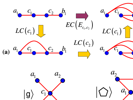
Fig. 1(b) and (c) shows two simple and important examples of graph states that are not equivalent under local-unitary transformations, the star $S_{N}$ and cycle $C_{N}$ graphs. The star graphs correspond to GHZ states:

$\displaystyle|S_{n}\rangle={1\over\sqrt{2^{n+1}}}(-1)^{q(x)}|x_{c_{1}}\,x_{a_{1}}\cdots x_{a_{n}}\rangle$ (5)

with $q(x)=\sum_{i=1}^{n}x_{c_{1}}x_{a_{i}}$; these are LC-equivalent to the complete graphs $K_{n+1}$. Fig. 1(b) depicts $|S_{4}\rangle\equiv|g\rangle$. The cycle graph state is equal to

$\displaystyle|C_{N}\rangle={1\over\sqrt{2^{N}}}(-1)^{r(x)}|x_{a_{1}}\cdots x_{a_{N}}\rangle$ (6)

with $r(x)=x_{a_{1}}x_{a_{N}}+\sum_{i=2}^{N-1}x_{a_{i}}x_{a_{i+1}}$. Fig. 1(c) shows $|C_{5}\rangle\equiv|\pentagon\rangle$. The former is related to classically encoded graph states and the latter to 5QECC [13].

Local complementation and edge local complementation are two operations used to classify locally-equivalent graphs that are generally inequivalent under isomorphism (vertex permutation). The action of local complementation $LC(a)$ at the vertex $a$ transforms the graph $G$ by replacing the subgraph associated with the neighboring vertices ${\mathcal{N}}(a)$ by its complement [11]. The new graph generated by $LC(a)$ on $G$ is locally equivalent to the original graph. It is important to note that the $LC(a)$ operation does not affect the edges of outer vertices in the graph $G$; only the neighborhood of vertex $a$ is affected. The action of edge local complementation $ELC(a,b)$ on the edge $\{a,b\}\in E$ is defined by three local complementations: $ELC(a,b)=LC(a)\,LC(b)\,LC(a)=LC(b)\,LC(a)\,LC(b)$. The action of ELC on the edge $\{a,b\}$ can be understood as follows. Consider any pair of vertices $\{c,d\}\in E$, where $c$ is a neighbor of $a$ but not $b$ and $d$ is a neighbor of $b$ but not $a$ (or vice versa); alternatively, $c$ and $d$ can both be neighbors of $a$ and $b$. ELC then corresponds to complementing the edge between $c$ and $d$, i.e. if $\{c,d\}\in E$ then delete the edge, and add it if $\{c,d\}\notin E$. In addition, the neighborhoods of $a$ and $b$ are replaced with one another. Edge local complementation has been investigated for recognizing the edge locally equivalence of two graphs [14] and for understanding the relationship between classical codes and graphs [15].

In the context of graph states, local equivalence implies that one graph state can be transformed into another by the action of single-qubit (i.e. local) operations. It is well-known that two graph states that are equivalent under stochastic local operations and classical communication (SLOCC) must also be equivalent under the local unitary (LU) operations [16]. A long-standing conjecture held that LU equivalence also implied equivalence under the action of Clifford-group elements (operations that map the Pauli group to itself), though this was recently proved to be false in general [17].

Nevertheless, the transformations $LC$ (and therefore $ELC$) on graph states can be expressed solely in terms of local Clifford operations [2]:

$$LC(a)=\sqrt{-\imath X_{a}}\bigotimes_{b={\mathcal{N}}(a)}\sqrt{\imath Z_{b}}\propto\sqrt{S(a)},$$ (7)

where $\imath\equiv\sqrt{-1}$. Suppose that $|G\rangle$ possesses qubit $c_{1}$ (called a core qubit) connected to $n$ neighboring qubits. The action of $LC(c_{1})$ corresponds to the application of ${n(n-1)\over 2}$ $CZ$ operations on the graph state, creating edges between ${\mathcal{N}}(c_{1})$ if there were none and removing them otherwise ($CZ^{2}=I$). Although entanglement between the two graph states is the same due to the invariance of entanglement under local unitary operations, the number of effective $CZ$ operations (i.e. the number of edges) differs. Edge local complementation on the edge $\{a,b\}$ would then correspond to the operation

$$ELC(a,b)=\sqrt{-\imath X_{a}}\bigotimes_{c={\mathcal{N}}(a)}\sqrt{\imath Z_{c}}\sqrt{-\imath X_{b}}\bigotimes_{d={\mathcal{N}}^{\prime}(b)}\sqrt{\imath Z_{d}}\sqrt{-\imath X_{a}}\bigotimes_{f={\mathcal{N}}^{\prime\prime}(a)}\sqrt{\imath Z_{f}},$$ (8)

where the ${\mathcal{N}}^{\prime}$ and ${\mathcal{N}}^{\prime\prime}$ are reminders that the neighborhoods themselves change under the $LC$ operations. Recognizing that $a$ and $b$ remain neighbors, this can be rewritten

$$ELC(a,b)=(-\imath)H_{a}\otimes H_{b}\bigotimes_{c={\mathcal{N}}(a)\backslash b}\sqrt{\imath Z_{c}}\bigotimes_{d={\mathcal{N}}^{\prime}(b)\backslash a}\sqrt{\imath Z_{d}}\bigotimes_{f={\mathcal{N}}^{\prime\prime}(a)\backslash b}\sqrt{\imath Z_{f}},$$ (9)

where $H_{a}=(X_{a}+Z_{a})/\sqrt{2}=\sqrt{-\imath X_{a}}\sqrt{\imath Z_{a}}\sqrt{-\imath X_{a}}$ is the Hadamard operator on qubit $a$. One of the goals of this manuscript is to show that the result of this operation on graph states can be expressed in the simpler form $ELC(a,b)|G\rangle=H_{a}\otimes H_{b}|G\rangle$, requiring the application of far fewer local operations.

Simple examples of LC and ELC are shown in Fig. 1(a). The initial graph state $|G\rangle$ consists of four qubits and three edges. After the first $LC(c_{1})$, because no edge exists between two neighboring qubits of $c_{1}$ in state $|G\rangle$, an edge is drawn between them. After $LC(c_{2})$, the edge on qubits $a_{1}$ and $c_{1}$ is deleted by a rule of the local complementation because two sequential $CZ$ operations become the identity between $a_{1}$ and $c_{1}$. Finally, after the last $LC(c_{1})$, the number of edges are four on the final graph state, which is represented by $ELC(c_{1},c_{2})|G\rangle$, although all four graph states are locally equivalent.

3 Edge local complementation via Hadamard gates

Consider two disconnected graphs $G_{1}=(V_{1},E_{1})$ and $G_{2}=(V_{2},E_{2})$ and their respective graph states states $|G_{1}\rangle$ and $|G_{2}\rangle$; each possesses a core vertex (qubit) $c_{1}\in V_{1}$ and $c_{2}\in V_{2}$, respectively. A $CZ$ operation is then applied to the two core qubits, linking the two graph states into a single connected graph $|G_{u}\rangle=CZ_{c_{1},c_{2}}|G_{1}\rangle\otimes|G_{2}\rangle$. If a Hadamard operation is then applied to each core qubit, the graph $|G_{u}\rangle$ is transformed into another locally equivalent graph state $|G_{H}\rangle=H_{c_{1}}\otimes H_{c_{2}}|G_{u}\rangle$. Below we show that the state $|G_{H}\rangle$ is the edge local complement of $|G_{u}\rangle$, i.e. that $|G_{H}\rangle=H_{c_{1}}\otimes H_{c_{2}}|G_{u}\rangle=ELC(c_{1},c_{2})|G_{u}\rangle$. It is important to note that the equivalence of edge complementation on $\{c_{1},c_{2}\}\in E$ with the application of Hadamard operations on $c_{1}$ and $c_{2}$ is only valid if ${\mathcal{N}}(c_{1})\backslash c_{2}\cap{\mathcal{N}}(c_{2})\backslash c_{1}=0$, i.e. that prior to the application of $CZ_{c_{1},c_{2}}$, the neighborhoods of $c_{1}$ and $c_{2}$ were completely disjoint. Our results do not apply to graphs where $c_{1}$ and $c_{2}$ share a neighborhood (other than themselves).

The main theorem of the paper is the following:

Theorem 3.1.

Consider two graph states $|G_{1}\rangle={1\over\sqrt{2^{N_{1}}}}(-1)^{\sum_{i\neq j}A_{ij}^{(1)}x_{i}x_{j}}|x_{1}\cdots x_{N_{1}}\rangle$ and $|G_{2}\rangle={1\over\sqrt{2^{N_{2}}}}(-1)^{\sum_{i\neq j}A_{ij}^{(2)}x_{i}x_{j}}|x_{1}\cdots x_{N_{2}}\rangle$, defined by adjacency matrices $A^{(1)}$ and $A^{(2)}$ on independent vertex sets $V_{1}\in\{a_{1}^{(1)},\ldots,a_{N_{1}}^{(1)}\}$ and $V_{2}\in\{a_{1}^{(2)},\ldots,a_{N_{2}}^{(2)}\}$, respectively. If core qubits, $c_{1}$ and $c_{2}$, are chosen at random from each of these vertex sets, and are entangled with one another by means of a $CZ$ gate, then

$$H_{c_{1}}H_{c_{2}}CZ_{c_{1},c_{2}}|G_{1}\rangle|G_{2}\rangle=ELC(c_{1},c_{2})CZ_{c_{1},c_{2}}|G_{1}\rangle|G_{2}\rangle,$$ (10)

where the edge local complementation operator on the edge $\{c_{1},c_{2}\}$ is $ELC(c_{1},c_{2})=LC(c_{1})LC(c_{2})LC(c_{1})$, and the (vertex) local complementation operator at qubit $a$ complements the edge set of its neighborhood ${\mathcal{N}}(a)$.

Proof.

The core qubits $c_{1}$ and $c_{2}$ have neighborhood ${\mathcal{N}}(c_{1})=\{b_{1}^{(1)},\ldots,b_{n}^{(1)}\}$ and ${\mathcal{N}}(c_{2})=\{b_{1}^{(2)},\ldots,b_{m}^{(2)}\}$), respectively. The remaining vertices of the graphs $G_{1}\rangle$ and $G_{2}\rangle$ are $V_{1}\backslash\{c_{1},b_{1}^{(1)},\ldots,b_{n}^{(1)}\}=\{o_{1}^{(1)},\ldots o_{N_{1}-n-1}^{(1)}\}\in V_{1}$ and $V_{2}\backslash\{c_{2},b_{1}^{(2)},\ldots,b_{m}^{(2)}\}=\{o_{1}^{(2)},\ldots o_{N_{2}-m-1}^{(2)}\}\in V_{2}$, respectively. Performing a $CZ$ operation between these core qubits, the graph state $|G_{u}\rangle$ is

$\displaystyle|G_{u}\rangle$ $\displaystyle=$ $\displaystyle CZ_{c_{1},c_{2}}|G_{1}\rangle|G_{2}\rangle=(-1)^{x_{c_{1}}x_{c_{2}}}|G_{1}\rangle|G_{2}\rangle,$ (11)
$\displaystyle=$ $\displaystyle\frac{(-1)^{x_{c_{1}}x_{c_{2}}}}{\sqrt{2^{N_{1}+N_{2}}}}(-1)^{\left(q_{1}(x)+q_{2}(x)\right)}|x_{a_{1}^{(1)}}\cdots x_{a_{N_{1}}^{(1)}}\rangle|x_{a_{1}^{(2)}}\cdots x_{a_{N_{2}}^{(2)}}\rangle,$
$$q_{1}(x)=\sum_{i\neq j}A_{ij}^{(1)}x_{a_{i}^{(1)}}x_{a_{j}^{(1)}}=x_{c_{1}}\sum_{i=1}^{n}x_{b_{i}^{(1)}}+\sum_{i\neq j}A_{ij}^{(1)}x_{o_{i}^{(1)}}x_{o_{j}^{(1)}};$$ (12)
$$q_{2}(x)=\sum_{i\neq j}A_{ij}^{(2)}x_{a_{i}^{(2)}}x_{a_{j}^{(2)}}=x_{c_{2}}\sum_{i=1}^{m}x_{b_{i}^{(2)}}+\sum_{i\neq j}A_{ij}^{(2)}x_{o_{i}^{(2)}}x_{o_{j}^{(2)}}.$$ (13)

3.1 Two Hadamards applied to core qubits

Consider

$$|G_{H}\rangle=H_{c_{1}}H_{c_{2}}|G_{u}\rangle=\frac{1}{2}\left(X_{c_{1}}X_{c_{2}}+X_{c_{1}}Z_{c_{2}}+Z_{c_{1}}X_{c_{2}}+Z_{c_{1}}Z_{c_{2}}\right)|G_{u}\rangle.$$ (14)

This can be simplified by noting that for $b_{j}\in{\mathcal{N}}(c_{1})$

$\displaystyle X_{c_{1}}(-1)^{x_{c_{1}}x_{b_{j}}}$ $\displaystyle=$ $\displaystyle(-1)^{(x_{c_{1}}+1)x_{b_{j}}}X_{c_{1}};$
$\displaystyle Z_{c_{1}}(-1)^{x_{c_{1}}x_{b_{j}}}$ $\displaystyle=$ $\displaystyle(-1)^{x_{c_{1}}}(-1)^{x_{c_{1}}x_{b_{j}}}=(-1)^{x_{c_{1}}(x_{b_{j}}+1)}.$ (15)

One then obtains

$\displaystyle H_{c_{1}}H_{c_{2}}(-1)^{x_{c_{1}}x_{c_{2}}}$ $\displaystyle=$ $\displaystyle\frac{1}{2}(-1)^{x_{c_{1}}x_{c_{2}}}\Big{[}-(-1)^{(x_{c_{1}}+x_{c_{2}})}X_{c_{1}}X_{c_{2}}$ (16)
$\displaystyle+$ $\displaystyle X_{c_{1}}+X_{c_{2}}+(-1)^{(x_{c_{1}}+x_{c_{2}})}\Big{]}.$

Applying this to the remaining operators in Eq. (11) gives

$\displaystyle|G_{H}\rangle$ $\displaystyle=$ $\displaystyle\frac{(-1)^{x_{c_{1}}x_{c_{2}}}}{\sqrt{2^{N_{1}+N_{2}}}}(-1)^{\left(q_{1}(x)+q_{2}(x)\right)}\frac{1}{2}\prod_{k,k^{\prime}}\Big{[}-(-1)^{(x_{c_{1}}+x_{c_{2}}+x_{b_{k}^{(1)}}+x_{b_{k^{\prime}}^{(2)}})}$ (17)
$\displaystyle+$ $\displaystyle(-1)^{x_{b_{k}^{(1)}}}+(-1)^{x_{b_{k^{\prime}}^{(2)}}}+(-1)^{(x_{c_{1}}+x_{c_{2}})}\Big{]}|x_{a_{1}^{(1)}}\cdots x_{a_{N_{1}}^{(1)}}\rangle|x_{a_{1}^{(2)}}\cdots x_{a_{N_{2}}^{(2)}}\rangle$
$\displaystyle=$ $\displaystyle\frac{(-1)^{x_{c_{1}}x_{c_{2}}}}{\sqrt{2^{N_{1}+N_{2}}}}(-1)^{\left(q_{1}(x)+q_{2}(x)+q_{3}(x)\right)}|x_{a_{1}^{(1)}}\cdots x_{a_{N_{1}}^{(1)}}\rangle|x_{a_{1}^{(2)}}\cdots x_{a_{N_{2}}^{(2)}}\rangle,$

where

$$q_{3}(x)=\left(x_{c_{1}}+x_{c_{2}}\right)\left(\sum_{k}x_{b_{k}^{(1)}}+\sum_{k^{\prime}}x_{b_{k^{\prime}}^{(2)}}\right)+\sum_{k,k^{\prime}}x_{b_{k}^{(1)}}x_{b_{k^{\prime}}^{(2)}}.$$ (18)

Finally, one can combine all the terms to obtain

$\displaystyle|G_{H}\rangle=H_{c_{1}}H_{c_{2}}CZ_{c1,c2}|G_{1}\rangle|G_{2}\rangle=\frac{(-1)^{p(x)}}{\sqrt{2^{N_{1}+N_{2}}}}|x_{a_{1}^{(1)}}\cdots x_{a_{N_{1}}^{(1)}}\rangle|x_{a_{1}^{(2)}}\cdots x_{a_{N_{2}}^{(2)}}\rangle,$ (19)

where

$\displaystyle p(x)$ $\displaystyle=$ $\displaystyle x_{c_{1}}x_{c_{2}}+x_{c_{1}}\sum_{k^{\prime}=1}^{m}x_{b_{k^{\prime}}^{(2)}}+x_{c_{2}}\sum_{k=1}^{n}x_{b_{k}^{(1)}}+\sum_{k=1}^{n}\sum_{k^{\prime}=1}^{m}x_{b_{k}^{(1)}}x_{b_{k^{\prime}}^{(2)}}$ (20)
$\displaystyle+$ $\displaystyle\sum_{i\neq j}A_{ij}^{(1)}x_{o_{i}^{(1)}}x_{o_{j}^{(1)}}+\sum_{i\neq j}A_{ij}^{(2)}x_{o_{i}^{(2)}}x_{o_{j}^{(2)}}.$

3.2 Edge local complementation on core qubits

Recall that edge local complementation $ELC(c_{1},c_{2})$ on the edge $\{c_{1},c_{2}\}$ is described by the three local complementations $LC(c_{1})LC(c_{2})LC(c_{1})=LC(c_{2})LC(c_{1})LC(c_{2})$. Suppose that the first local complementation is performed on $|G_{u}\rangle$ at qubit $c_{1}$. The result is that all neighboring qubits of $c_{1}$ are explicitly connected to each other (adding an edge to an existing edge annihilates it). The additional edges are given by the quadratic form

$$r_{1}(x)=\sum_{i\neq j}x_{b_{i}^{(1)}}x_{b_{j}^{(1)}}+x_{c_{2}}\sum_{i}x_{b_{i}^{(1)}}.$$ (21)

Next one complements the neighborhood of qubit $c_{2}$, which is given by the quadratic form $x_{c_{2}}\left(x_{c_{1}}+\sum_{i}x_{b_{i}^{(1)}}+\sum_{i}x_{b_{i}^{(2)}}\right)$; the result is $x_{c_{1}}\left(\sum_{i}x_{b_{i}^{(1)}}+\sum_{i}x_{b_{i}^{(2)}}\right)+\sum_{i\neq j}x_{b_{i}^{(1)}}x_{b_{j}^{(1)}}+\sum_{i\neq j}x_{b_{i}^{(2)}}x_{b_{j}^{(2)}}+\sum_{i,j}x_{b_{i}^{(1)}}x_{b_{j}^{(2)}}$. The total additional edges are then given by the quadratic form

$\displaystyle r_{2}(x)$ $\displaystyle=$ $\displaystyle x_{c_{2}}\sum_{i}x_{b_{i}^{(1)}}+x_{c_{1}}\left(\sum_{i}x_{b_{i}^{(1)}}+\sum_{i}x_{b_{i}^{(2)}}\right)+\sum_{i\neq j}x_{b_{i}^{(2)}}x_{b_{j}^{(2)}}$ (22)
$\displaystyle+$ $\displaystyle\sum_{i,j}x_{b_{i}^{(1)}}x_{b_{j}^{(2)}}.$

Last, one complements the neighborhood of qubit $c_{1}$, which is given by the quadratic form $x_{c_{1}}\left(x_{c_{2}}+\sum_{i}x_{b_{i}^{(1)}}+\sum_{i}x_{b_{i}^{(1)}}+\sum_{i}x_{b_{i}^{(2)}}\right)=x_{c_{1}}\left(x_{c_{2}}+\sum_{i}x_{b_{i}^{(2)}}\right)$; the result is simply $x_{c_{2}}\sum_{i}x_{b_{i}^{(2)}}+\sum_{i\neq j}x_{b_{i}^{(2)}}x_{b_{j}^{(2)}}$. The quadratic form for the additional edges after this final operation is

$\displaystyle r_{3}(x)$ $\displaystyle=$ $\displaystyle x_{c_{2}}\left(\sum_{i}x_{b_{i}^{(1)}}+\sum_{i}x_{b_{i}^{(2)}}\right)+x_{c_{1}}\left(\sum_{i}x_{b_{i}^{(1)}}+\sum_{i}x_{b_{i}^{(2)}}\right)$ (23)
$\displaystyle+$ $\displaystyle\sum_{i,j}x_{b_{i}^{(1)}}x_{b_{j}^{(2)}}.$

Combining this result with the remaining terms in the quadratic form (11), the graph resulting from the edge local complementation becomes

$$ELC(c_{1},c_{2})|G_{u}\rangle=\frac{(-1)^{p(x)}}{\sqrt{2^{N_{1}+N_{2}}}}|x_{a_{1}^{(1)}}\cdots x_{a_{N_{1}}^{(1)}}\rangle|x_{a_{1}^{(2)}}\cdots x_{a_{N_{2}}^{(2)}}\rangle,$$ (24)

where

$\displaystyle p(x)$ $\displaystyle=$ $\displaystyle x_{c_{1}}x_{c_{2}}+x_{c_{1}}\sum_{i}x_{b_{i}^{(2)}}+x_{c_{2}}\sum_{i}x_{b_{i}^{(1)}}+\sum_{i,j}x_{b_{i}^{(1)}}x_{b_{j}^{(2)}}$ (25)
$\displaystyle+$ $\displaystyle\sum_{i\neq j}A_{ij}^{(1)}x_{o_{i}^{(1)}}x_{o_{j}^{(1)}}+\sum_{i\neq j}A_{ij}^{(2)}x_{o_{i}^{(2)}}x_{o_{j}^{(2)}},$

which is identical to the quadratic form (20).

Eq. (20) shows that when Hadamard gates are applied to both (core) qubits of single edge between two graphs, the result is a new graph state corresponding to the effective application of $2(n+m)+nm$ controlled-phase operations. These operations have the effect of replacing the original neighborhood of each core qubit with the neighborhood of the other core qubit (and vice versa), while simultaneously adding the neighborhood of a given core qubit to the neighborhood of the other. That is, from the edge set one deletes the combinations $\{c_{1},b_{k}^{(1)}\}$ and $\{c_{2},b_{k}^{(2)}\}$, and adds the combinations $\{c_{1},b_{k}^{(2)}\}$, $\{c_{2},b_{k}^{(1)}\}$, and $\{b_{k}^{(1)},b_{k^{\prime}}^{(2)}\}$. In other words, the Hadamard operations have complemented the neighborhood of the edge $\{c_{1},c_{2}\}$, or performed edge local complementation. Of particular interest is the special case where both of the original graphs $|G_{1}\rangle$ and $|G_{2}\rangle$ were star graphs with the core qubit corresponding to the maximum-degree vertex, i.e. where $\{o_{i}^{(1)}\}\not\in V_{1}$ and $\{o_{i}^{(2)}\}\not\in V_{2}$. Then the resulting graph would be completely bipartite, with every vertex of the first group $\{c_{1},b_{1}^{(1)},\ldots,b_{n}^{(1)}\}$ connected to every vertex of the second group $\{c_{2},b_{1}^{(2)},\ldots,b_{n}^{(2)}\}$ [18].

3.3 Vertex local complementation

The above analysis proves that the application of Hadamard operations to the core qubits $c_{1}$ and $c_{2}$ is equivalent to edge local complementation on the edge $\{c_{1},c_{2}\}$. It is not obvious that edge local complementation based on the formal definition of local complementation given in Eq. (7), $LC(c_{1})=\sqrt{-\imath X_{c_{1}}}\prod_{b={\mathcal{N}}(c_{1})}\sqrt{\imath Z_{b}}$, reproduces the same result. Though graph transformations effected by this expression have already been discussed in Ref. [2] in the context of vertex local complementation, edge local complementation using this operator was not explicitly explored in that work. In fact, as shown below, the application of these unitary gates in order to effect edge local complementation requires local operations in addition to the two Hadamard gates.

It is convenient to write

$$\sqrt{-\imath X}=[-I+\imath X]/\sqrt{2};\quad\sqrt{\imath Z}=[\imath I+Z]/\sqrt{2}.$$ (26)

The action of these on quadratic forms is

$\displaystyle\sqrt{-\imath X_{c_{1}}}(-1)^{x_{c_{1}}x_{b_{j}}}$ $\displaystyle=$ $\displaystyle(-1)^{x_{c_{1}}x_{b_{j}}}\left[-1+i(-1)^{x_{b_{j}}}X_{c_{1}}\right]/\sqrt{2};$
$\displaystyle\sqrt{\imath Z_{b_{j}}}(-1)^{x_{c_{1}}x_{b_{j}}}$ $\displaystyle=$ $\displaystyle(-1)^{x_{c_{1}}x_{b_{j}}}\left[\imath+(-1)^{x_{b_{j}}}\right]/\sqrt{2}.$ (27)

Suppose one has an arbitrary graph state $|G\rangle$ defined by quadratic form $p(x)$ whose neighborhood of the qubit $c_{1}$ is ${\mathcal{N}}(c_{1})=\{b_{1},\ldots,b_{n}\}$, i.e. where $p(x)$ includes the term $c_{1}\sum_{j}b_{j}$. Local complementation on the vertex $c_{1}$ then yields

$\displaystyle LC(c_{1})$ $\displaystyle=$ $\displaystyle\sqrt{-\imath X_{c_{1}}}\prod_{j=1}^{n}\sqrt{\imath Z_{b_{j}}}(-1)^{x_{c_{1}}x_{b_{j}}}$
$\displaystyle=$ $\displaystyle\frac{1}{2^{n/2}}\sqrt{-\imath X_{c_{1}}}\prod_{j=1}^{n}(-1)^{x_{c_{1}}x_{b_{j}}}\left[\imath+(-1)^{x_{b_{j}}}\right]$
$\displaystyle=$ $\displaystyle{1\over 2^{n}}\prod_{j=1}^{n}(-1)^{x_{c_{1}}x_{b_{j}}}\left[\imath+(-1)^{x_{b_{j}}}\right]\left[-1+i(-1)^{x_{b_{j}}}X_{c_{1}}\right].$

When this local complementation operator is applied to the graph state $|G\rangle$, the $X_{c_{1}}$ operator will act only on its eigenstates and will effectively disappear. The effect of the various terms above is then equivalent to the new quadratic form

$$p(x)^{\prime}=p(x)+\sum_{j\neq k}b_{j}b_{k}-\sum_{i}b_{i}.$$ (28)

In other words, $LC(c_{1})$ has complemented the neighborhood of qubit $c_{1}$, by effectively applying $CZ$ entangling operations to all of its neighbors. In addition, it has applied $Z$ gates to all the neighbors. These are local operations that commute with the $CZ$s and are therefore unimportant. That said, complete equivalence (rather than simply unitary equivalence) under edge local complementation would then require the application of additional unitary gates beyond the two Hadamard gates.

4 Application : Efficient generation of 1D logical cluster states

We now discuss a novel and useful application of the theory of edge local complementation for quantum information processing. In previous work [6], we showed that logical cluster states corresponding to 5QECC can be made with logical $CZ$ operations consisting of many $CZ$ operations among the physical qubits. A linear $N$-qubit logical cluster state is given by

$$|CS^{L}_{N}\rangle=\prod_{i=1}^{N-1}CZ^{L}_{i\,i+1}|+^{L}\rangle_{1}\otimes\cdots\otimes|+^{L}\rangle_{N},$$ (29)

where $CZ^{L}$ is a logical $CZ$ operation between two logical qubits and $|\pm^{L}\rangle=(|0^{L}\rangle\pm|1^{L}\rangle)/\sqrt{2}$. For $|CS^{L}_{2}\rangle$ with 5QECC, 25 physical $CZ$ operations are required to construct a logical $CZ$ operation from $|+\rangle^{\otimes 10}$ (see Fig. 3 in Ref. [6]). The construction of many-qubit logical cluster states requires so many entangling operations to build logical $CZ$ gates as to be impractical for realistic quantum information processing. In this context, the edge local complementation provides an efficient solution to this conundrum: a single physical $CZ$ operation and two Hadamard operations are sufficient to build a logical $CZ$ operation between two logical qubits.

First we will review how to encode a physical qubit into a logical qubit with 5QECC. One begins begin with a qubit in state $|0\rangle_{a_{1}}$ and four auxiliary qubits in $|++++\rangle_{a_{2}-a_{5}}$. After a Hadamard operation on qubit $a_{1}$ and four $CZ$ operations between $a_{1}$ and the others, one obtains the five-qubit GHZ-type graph state $|g\rangle_{A}$ (see Fig. 1(b) but with $c_{1}$ replaced by $a_{1}$ and $a_{1,2,3,4}$ replaced by $a_{2,3,4,5}$). After an additional Hadamard operation on qubit $a_{1}$ in $|g\rangle_{A}$, the state is equal to a five-qubit GHZ state

$\displaystyle|g^{+}_{H}\rangle_{A}={1\over\sqrt{2}}\big{(}|+\rangle^{\otimes 5}_{a_{1}-a_{5}}+|-\rangle^{\otimes 5}_{a_{1}-a_{5}}\big{)},$ (30)

$|\pm\rangle^{\otimes 5}_{a_{1}-a_{5}}=|\pm\rangle_{a_{1}}|\pm\rangle_{a_{2}}|\pm\rangle_{a_{3}}|\pm\rangle_{a_{4}}|\pm\rangle_{a_{5}}$. Because $|0\rangle_{a_{1}}=(|+\rangle_{a_{1}}+|-\rangle_{a_{1}})/\sqrt{2}$, the state $|g^{+}_{H}\rangle$ can be understood as a classically encoded state of $|0\rangle_{a_{1}}$ in five qubits (here a classical encoding is meant to signify the implementation of a repetition code $|\pm\rangle\rightarrow|\pm\rangle^{\otimes 5}$). Similarly, if the physical qubit is initialized in $|1\rangle_{a_{1}}$, the outcome state is $|g^{-}_{H}\rangle_{A}=\big{(}|+\rangle^{\otimes 5}_{a_{1}-a_{5}}-|-\rangle^{\otimes 5}_{a_{1}-a_{5}}\big{)}/\sqrt{2}$. The quantum encoding scheme transforms $|+\rangle^{\otimes 5}_{A}$ into $|+^{L}\rangle_{A}$ and $|-\rangle^{\otimes 5}_{A}$ into $|-^{L}\rangle_{A}$. As shown in Fig. 1(c), a pentagon graph operation is used for encoding logical qubits

$\displaystyle|+^{L}\rangle_{A}$ $\displaystyle\equiv$ $\displaystyle|\pentagon\rangle_{A}=C^{\pentagon}_{a_{1}-a_{5}}|+\rangle^{\otimes 5}_{a_{1}-a_{5}},$ (31)
$\displaystyle|-^{L}\rangle_{A}$ $\displaystyle\equiv$ $\displaystyle|\tilde{\pentagon}\rangle_{A}=C^{\pentagon}_{a_{1}-a_{5}}|-\rangle^{\otimes 5}_{a_{1}-a_{5}}=\prod^{5}_{i=1}Z_{i}|+^{L}\rangle_{A},$ (32)

where $C^{\pentagon}_{a_{1}-a_{5}}=CZ_{a_{1},a_{2}}\,CZ_{a_{2},a_{3}}\,CZ_{a_{3},a_{4}}\,CZ_{a_{4},a_{5}}\,CZ_{a_{5},a_{1}}$. Therefore, the total encoding operation for a logical qubit is represented by

$\displaystyle E^{L}_{A}=C^{\pentagon}_{a_{1}-a_{5}}\,H_{a_{1}}\,\left[\prod_{i=2}^{5}CZ_{a_{1},a_{i}}\right]\,H_{a_{1}},$ (33)

and $|\pm^{L}\rangle_{A}=E^{L}_{A}|\pm\rangle_{a_{1}}|+\rangle^{\otimes 4}_{a_{2}-a_{5}}$.

Refer to caption
Figure 2: The edge local complementation consisting of three sequential local complementations makes the same transformation as the operation of two Hadamard operations on core qubits. Green lines indicate new edges created by each local complementation while red lines do the pre-existing edges. The graph state $|G_{H}\rangle$ is completely bipartite.

With this toolkit one can show how to build logical cluster states. There are two different ways of building a two-qubit logical cluster state from ten physical qubits $|+\rangle^{\otimes 10}$. The first method is to first prepare two logical states in $|+^{L}\rangle$, and then to directly perform a logical $CZ$ operation between them:

$\displaystyle|CS^{L}_{2}\rangle_{AB}=CZ^{L}_{AB}\,E^{L}_{A}\,E^{L}_{B}|+\rangle^{\otimes 10}=CZ^{L}_{AB}|+^{L}\rangle_{A}|+^{L}\rangle_{B}.$ (34)

Because $E^{L}_{A}E^{L}_{B}|+\rangle^{\otimes 10}=C^{\pentagon}_{A}C^{\pentagon}_{B}|+\rangle^{\otimes 10}$ for this case, 35 physical $CZ$ operations in total are required to build $|CS^{L}_{2}\rangle$ from $|+\rangle^{\otimes 10}$ (for details refer to Ref. [6]).

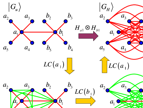
In the second method, one creates classically encoded graph states by means of edge local complementations; the quantum encoding is then applied to the classically encoded states to obtain logical cluster states. Initially, the core qubit $a_{1}$ of one classical state is entangled with its counterpart $b_{1}$ in the other state, yielding a two-qubit cluster state $|CS_{2}\rangle_{a_{1}b_{1}}=(|0\rangle_{a_{1}}|+\rangle_{b_{1}}+|1\rangle_{a_{1}}|-\rangle_{b_{2}})/\sqrt{2}$. Note that the first Hadamard operations $(H_{a_{1}}\otimes H_{b_{1}})$ in $E^{L}_{A}E^{L}_{B}$ leave the state $|CS_{2}\rangle_{a_{1}b_{1}}$ invariant. After the GHZ-type $CZ$ operations are performed between $a_{1}$ ($b_{1}$) and $a_{i}$ ($b_{i}$) ($i=2,3,4,5$), through the operation $\prod_{i}\prod_{j}CZ_{a_{1},a_{i}}CZ_{b_{1},b_{j}}$, a connected graph state $|G_{u}\rangle$ is obtained (see Fig. 2). When two Hadamard operations are subsequently applied to $a_{1}$ and $b_{1}$ in $|G_{u}\rangle$, the resulting state is transformed to another graph state $|G_{H}\rangle$, given by

$\displaystyle|G_{H}\rangle_{AB}={1\over 2}\left[|+\rangle^{\otimes 5}_{a_{1}-a_{5}}\left(|+\rangle^{\otimes 5}_{b_{1}-b_{5}}+|-\rangle^{\otimes 5}_{b_{1}-b_{5}}\right)+|-\rangle^{\otimes 5}_{a_{1}-a_{5}}\left(|+\rangle^{\otimes 5}_{b_{1}-b_{5}}-|-\rangle^{\otimes 5}_{b_{1}-b_{5}}\right)\right].$ (35)

This state is a classically encoded two-qubit cluster state.

In Fig. 2, it is shown that the action of three local complementations on the core vertices $a_{1}$ and $b_{1}$ provides the desired $CZ$ operations among the physical qubits, reproducing the state (35). The resulting graph is known as a complete bipartite graph state [18]: each of the vertices in one neighborhood (corresponding to logical register A or B) is connected with all the vertices of the other neighborhood, and vice versa. While it is possible to construct $|G_{H}\rangle_{AB}$ directly by applying 25 $CZ$ operations starting with $|+\rangle^{\otimes 10}$, it can be efficiently made using only 9 $CZ$ operations plus two local operations. For the quantum encoding scheme, the final state is given by

$\displaystyle|CS^{L}_{2}\rangle_{AB}=C^{\pentagon}_{a_{1}-a_{5}}C^{\pentagon}_{b_{1}-b_{5}}|G_{H}\rangle_{AB}=E^{L}_{A}E^{L}_{B}CZ_{a_{1}b_{1}}|+\rangle^{\otimes 10}.$ (36)

Therefore, the state $|CS^{L}_{2}\rangle$ can be efficiently built by 19 $CZ$ operations with the help of two Hadamard operations, instead of 35 $CZ$ operations, and the logical $CZ$ operation expressed by

$\displaystyle CZ^{L}_{AB}\,E^{L}_{A}\,E^{L}_{B}=E^{L}_{A}\,E^{L}_{B}\,CZ_{a_{1}b_{1}}$ (37)

shows that a single physical $CZ$ operation is sufficient to create a logical $CZ$ operation between logical qubits.

While the encoding procedure for graph states is straightforward to implement, its interpretation in terms of edge local complementation is not obvious in general. For example, any encoding of a cluster state with an odd number of qubits is difficult to express in terms of edge local complementations, each requiring an even number of Hadamard operations. The interpretation of encoding linear $2N$-qubit cluster states through edge local complementation is straightforward, however.

Consider for example the linear four-qubit logical cluster state. First one assigns five qubits each to registers A, B, C, and D. After assigning a core qubit from each, designated $a_{1}$, $b_{1}$, $c_{1}$, and $d_{1}$, respectively, one prepares the linear four-qubit cluster state $|CS_{4}\rangle=CZ_{a_{1},b_{1}}CZ_{b_{1},c_{1}}CZ_{c_{1},d_{1}}|+\rangle^{\otimes 4}_{a_{1}-d_{1}}$. The encoding consists of acting on each register with $\prod_{J}E^{L}_{J}|CS_{4}\rangle|+\rangle^{\otimes 16}$ for $J=A,B,C,D$, where $E^{L}_{J}$ is given in Eq. (33). The first step is to perform four Hadamard operations on $|CS_{4}\rangle$. Applying two Hadamard operations on qubits $a_{1}$ and $b_{1}$, the intermediate graph state is equal to

$\displaystyle|\Psi_{inter}\rangle_{a_{1}-d_{1}}=ELC(a_{1},b_{1})|CS_{4}\rangle=CZ_{a_{1},b_{1}}CZ_{a_{1},c_{1}}CZ_{c_{1},d_{1}}|+\rangle^{\otimes 4}_{a_{1}-d_{1}}$ (38)

using the results of edge local complementation. Because $c_{1}$ and $d_{1}$ share an edge but their neighborhoods are disjoint, it is reasonable to associate the subsequent Hadamard operations on qubits $c_{1}$ and $d_{1}$ with another edge local complementation on the edge $\{c_{1},d_{1}\}$. The resulting state is equal to another linear four-qubit cluster state, but with the vertex labels permuted:

$$|CS_{4}^{\prime}\rangle=ELC(c_{1},d_{1})|\Psi_{inter}\rangle_{a_{1}-d_{1}}=CZ_{a_{1},b_{1}}CZ_{a_{1},d_{1}}CZ_{c_{1},d_{1}}|+\rangle^{\otimes 4}_{a_{1}-d_{1}}.$$ (39)

After four GHZ-type operations and the second set of four Hadamard operations on $|CS_{4}^{\prime}\rangle_{a_{1}-d_{1}}|+\rangle^{\otimes 16}$, again corresponding to two edge local complementations, the outcome is a linear four-qubit cluster state with classical encoding. The Hadamard operations not only effect the edge local complementation; they also reverse the permutation of the vertex labels above. Finally, the quantum encoding scheme on all the qubits yields a logical four-qubit cluster state $|CS^{L}_{4}\rangle$, which is sufficient for universal quantum computation with 5QECC [6]. This procedure can be trivially extended to any even-length chain, by applying Hadamard gates in pairs on nearest-neighbor edges in order to implement edge local complementations from the left boundary of the chain to the right.

5 Summary and Remarks

The main result presented in this manuscript is a proof that the action of edge local complementation on a graph state can be effected solely through the use of two Hadamard operations applied to the edge qubits. A crucial assumption in this proof is that the neighborhoods of the edge qubits were disjoint, i.e. that the neighbors ${\mathcal{N}}(a)$ of the first edge qubit $a$ were different from the neighbors ${\mathcal{N}}(b)$ of the second qubit $b$. Under this restriction, edge local complementation interchanges the respective neighborhoods, i.e. ${\mathcal{N}}(a)\leftrightarrow{\mathcal{N}}(b)$, while simultaneously making neighbors of all the neighbors. In principle, this transformation would require a large number of either local unitary operations on the graph-state qubits or entangling gates between various qubits. The distinct advantage of the present scheme is the large savings in the number of (local) operations required.

As an example of the utility of this insight, we show how edge local complementation can be used to efficiently create classically encoded cluster states and one-dimensional logical cluster states based on the five-qubit error-correcting code, for an even number of logical qubits. In this scheme, a physical $CZ$ operation, together with local operations, is sufficient to create a logical $CZ$ operation between two logical qubits.

Arbitrary encoded graph states can be obtained by a straightforward extension of the procedure described above. The operations encoding a logical qubit, Eq. (33), are local to the physical qubits comprising the logical qubit, and therefore commute with one another. It therefore suffices to first construct the desired graph state with the core qubits, associate four ancillae to each core qubit, and operate independently with Eq. (33) on each five-qubit register.

Multipartite entangled states that fundamentally include fault tolerance might be desirable for practical measurement-based quantum computing and multipartite quantum communication [8, 19]. For a generalized scheme of level-$l$ logical graph states based on our proposal, the same encoding procedure can be used repeatedly. Since the level-1 logical graph state is made by our protocol, a level-$l$ concatenated logical graph state becomes an initial state to create a level-($l$+1) concatenated one ($|\pm^{L}_{l}\rangle\rightarrow|\pm^{L}_{l+1}\rangle$) with the help of the classical and quantum coding schemes described above. This concatenated method may also be useful for building multi-party quantum networks similar to classical complex networks in hierarchical organization [20].

Acknowledgements

The authors are grateful to T. P. Spiller and Jinhyoung Lee for stimulating discussions. This work was supported by the Natural Sciences and Engineering Research Council of Canada, the Mathematics of Information Technology and Complex Systems Quantum Information Processing Project, and the Quantum Interfaces, Sensors, and Communication based on Entanglement Integrating Project.

References

References

  • [1] R Horodecki, P Horodecki, M Horodecki, and K Horodecki (2009) Quantum entanglement Rev. Mod. Phys. 81 865, and references therein
  • [2] M Hein, J Eisert, and H J Briegel (2004) Multiparty entanglement in graph states Phys. Rev. A 69 062311; M Van den Nest, J Dehaene, and B De Moor (2004) Graphical description of the action of local Clifford transformations on graph states Phys. Rev. A 69 022316
  • [3] C-Y Lu, X-Q Zhou, O Gühne, W-B Gao, J Zhang, Z-S Yuan, A Goebel, T Yang, and J-W Pan (2007) Experimental entanglement of six photons in graph states Nat. Phys. 3 91; W-B Gao, C-Y Lu, X-C Yao, P Xu, O Gühne, A Goebel, Y-A Chen, C-Z Peng, Z-B Chen, and J-W Pan (2010) Experimental demonstration of a hyper-entangled ten-qubit Schrödinger cat state Nat. Phys. 6 331
  • [4] M A Nielsen and I L Chuang (2001) Quantum Computation and Quantum Information (Cambridge: Cambridge University Press), and references therein
  • [5] M Silva, V Danos, E Kashefi, and H Ollivier (2007) A direct approach to fault-tolerance in measurement-based quantum computation via teleportation New J. Phys. 9 192
  • [6] J Joo and D L Feder (2009) Error-correcting one-way quantum computation with global entangling gates Phys. Rev. A 80 032312
  • [7] K Fujii and K Yamamoto (2010) Cluster-based architecture for fault-tolerant quantum computation Phys. Rev. A 81 042324
  • [8] S Beigi, I Chuang, M Grassl, P Shor, and B Zeng (2011) Graph Concatenation for Quantum Codes J. Math. Phys. 52, 022201
  • [9] R Raussendorf and J Harrington (2007) Fault-Tolerant Quantum Computation with High Threshold in Two Dimensions Phys. Rev. Lett. 98 190504; R Raussendorf, J Harrington, and K Goyal (2007) Topological fault-tolerance in cluster state quantum computation New J. Phys. 9 199
  • [10] A Bouchet (1988) Graphic presentations of isotropic systems J. Combin. Theory Ser. B 45 58
  • [11] H. de Fraysseix (1981) Local complementation and interlacement graphs Discrete Math. 33 29
  • [12] A Cosentino and S Severini (2009) Weight of quadratic forms and graph states Phys. Rev. A 80 052309; J Dehaene and B De Moor (2003) Clifford group, stabilizer states, and linear and quadratic operations over GF(2) Phys. Rev. A 68 042318
  • [13] C H Bennett, D P DiVincenzo, J A Smolin, and W K Wootters (1996) Mixed-state entanglement and quantum error correction Phys. Rev. A 54 3824
  • [14] M Van den Nest and B De Moor (2005) Edge-local equivalence of graphs arXiv:math/0510246
  • [15] L E Danielsen, M G Parker, C Riera, J G Knudsen (2010) On Graphs and Codes Preserved by Edge Local Complementation arXiv:1006.5802; L E Danielsen and M G Parker (2008) Edge Local Complementation and Equivalence of Binary Linear Codes Des. Codes Cryptogr. 49 161
  • [16] M Van den Nest, J Dehaene, and B De Moor (2004) Local equivalence of stabilizer states Proceedings of the 16th International Symposium of Mathematical Theory of Networks and Systems (MTNS2004) (Belgium: Katholieke Universiteit Leuven)
  • [17] Z Ji, J Chen, Z Wei, and M Ying (2010) The LU-LC conjecture is false Quantum Inf. Comput. 10 97
  • [18] A Gibbon (1985) Algorithmic Graph Theory (Cambridge: Cambridge University Press)
  • [19] E Knill (2005) Quantum computing with realistically noisy devices Nature 434 39; E Knill (2005) Scalable quantum computing in the presence of large detected-error rates Phys. Rev. A 71 042322
  • [20] E Ravasz and A Barabási (2003) Hierarchical organization in complex networks Phys. Rev. E 67 026112