Modeling the multi-wavelength light curves of PSR B1259-63/SS 2883

Abstract

PSR B1259-63/SS 2883 is a binary system in which a 48-ms pulsar orbits around a Be star in a high eccentric orbit with a long orbital period of about 3.4 yr. Extensive broadband observational data are available for this system from radio band to very high energy (VHE) range. The multi-frequency emission is unpulsed and nonthermal, and is generally thought to be related to the relativistic electrons accelerated from the interaction between the pulsar wind and the stellar wind, where X-ray emission is from the synchrotron process and the VHE emission is from the inverse Compton (IC) scattering process. Here a shocked wind model with variation of the magnetization parameter $\sigma$ is developed for explaining the observations. By choosing proper parameters, our model could reproduce two-peak profile in X-ray and TeV light curves. The effect of the disk exhibits an emission and an absorption components in the X-ray and TeV bands respectively. We suggest that some GeV flares will be produced by Doppler boosting the synchrotron spectrum. This model can possibly be used and be checked in other similar systems such as LS I+61º303 and LS 5039.

1 Introduction

The discovery of the PSR B1259-63/SS 2883 system was first reported in 1992 (Johnston et al. 1992), and it is a binary system containing a rapidly rotating pulsar PSR B1259-63 in orbit around a massive Be star companion SS 2883. The spin period of the pulsar is $P$ = 47.76 ms and the spindown luminosity is $L_{\rm sp}\simeq 8\times 10^{35}$ ${\rm ergs}$ ${\rm s}^{-1}$. The distance between the system and Earth is estimated to be about 1.5 kpc (Johnston et al. 1994).

This system is special for having unpulsed and nonthermal multi-band observational data spanning from radio band to TeV range, which are variable along with the orbital phase (Johnston et al. 1994, 1996, 2005; Chernyakova et al. 2006, 2009; Uchiyama et al. 2009; Aharonian et al. 2005, 2009). The broadband emission from this system is generally believed to be produced by the ultrarelativistic electrons accelerated in the shock from the interaction between the pulsar wind and the outflow of Be star (Tavani & Arons 1997; Kirk, Ball & Skjæraasen 1999; Khangulyan et al. 2007; Takata & Taam 2009; Kerschhaggl 2010). Massive stars usually produce very strong stellar wind during their life time. For a Be star, the stellar wind is composed of two parts: a polar component and an equatorial component. The polar wind is faster and thinner; the equatorial component is slower and denser, and forms a disk surrounding the Be star. The interaction between the pulsar wind and the stellar outflow will form a termination shock at the position where the dynamical pressures of the pulsar wind and the stellar wind are in balance, and this shock will accelerate electrons to relativistic velocities. These accelerated electrons will emit nonthermal emission via synchrotron process for X-ray regime (Tavani & Arons 1997) or IC [either synchrotron self-Compton (SSC) or external inverse Compton scattering the thermal photons from the Be star (EIC)] process for VHE regime (Kirk, Ball & Skjæraasen 1999). So this system is an important astrophysical laboratory for studying the interaction between the pulsar wind and the stellar wind, and the nonthermal radiation arising from the shocked pulsar wind.

However, the prediction from a simple wind interaction model is not consistent with the observations. The simple wind interaction model predicts that the X-ray light curve reaches a maximum in flux at periastron (Tavani & Arons 1997), but the observed X-ray light curve has a two-peak profile and has a drop in photon flux around the periastron (Kaspi et al. 1995; Hirayama et al. 1999; Chernyakova et al. 2006, 2009). The behavior of TeV light curve is similar to that in X-ray range (Aharonian et al. 2005, 2009). Some authors suggest that hadronic scenarios may take place in the system (Kawachi et al. 2004; Neronov & Chernyakova 2007). In the hadronic model, The Ultra-high energy (UHE) protons will be produced by the interaction between the pulsar wind and the dense equatorial wind. These UHE protons can loose their energy in interactions with the protons from the stellar wind and produce pions. The decay of neutral pions will produce the TeV emission, and the leptons from the decay of charged pions will produce the radio to GeV emission via the synchrotron and IC processes respectively. In this situation, the two-peak profile in the light curve is related to the passage of the Be star disk. On the other hand, some other authors use some revised leptonic models to explain the drop of photon flux towards periastron (Kangulyan et al. 2007; Takata & Taam 2009). Kangulyan et al. (2007) suggest that the observed TeV light curve can be explained (i) by increasing of the adiabatic loss rate close to periastron or (ii) by the early sub-TeV cut-offs in the energy spectra of electrons due to the enhanced rate of Compton losses near the periastron. More recently, Takata & Taam (2009) explain the observed light curves by varying the microphysical parameters in two different ways: (i) they use a given power-law spectral index $p$ of electron distribution, and vary the magnetization parameter $\sigma$ and the pulsar wind bulk Lorentz factor $\Gamma$; (ii) the magnetization parameter and the power law index are varied for a given bulk Lorentz factor.

Among all the mechanisms, we believe that the variation of microphysics model needs to be paid particular attention, especially the variation of the magnetization parameter $\sigma$. The varying of the magnetization parameter $\sigma$ along with the distance from the pulsar is a very natural hypothesis. In the Crab Nebula, $\sigma\sim 0.003$ at a distance of $r_{\rm s}\sim 3\times 10^{17}$ cm (Kennel & Coroniti 1984a, 1984b). But at the light cylinder of a pulsar, $\sigma$ should be much larger and is about $10^{4}$ - $10^{5}$. Between the light cylinder and the termination shock, the magnetic energy will be gradually converted into the particle kinetic energy, and $\sigma$ will vary along with the energy transition. Especially, a larger $\sigma$ around periastron will decrease the energy in particles and make the cooling faster, which may cause a drop in photon flux.

The PSR B1259-63/SS 2883 system is also special for having a large eccentricity of $e=0.87$ and a long orbital period of about 3.4 yr. The semimajor axis of the orbit is about 5 AU. Although the wind interaction model for this binary system is very similar to the pulsar wind nebulae (PWN) model (Kennel & Coroniti 1984a, 1984b), the detailed situation is different. For the PWN around an isolated pulsar like Crab, the distance between the pulsar and the termination shock $r_{\rm s}$ is about 0.1 pc and the magnetic parameter $\sigma$ is about 0.003 (Kennel & Coroniti 1984a, 1984b). However, in the case of PSR B1259-63/SS 2883 system, due to the highly eccentric orbit, $r_{\rm s}$ is in the range of 0.1 - 1 AU and $\sigma$ should be accordingly larger. This gives us the unique opportunity to study the physical properties of the pulsar wind near the light cylinder where $\sigma$ is much higher.

In this paper we develop a simple shocked wind model, in which the magnetization parameter $\sigma$ varies with $r_{\rm s}$ to reproduce the broadband observational data. Besides PSR B1259-63/SS 2883, there are also some other similar binary systems being found for emitting the X-ray and VHE emission, such as LS I+61º303 (Albert et al. 2006) and LS 5039 (Aharonian et al. 2006). We suggest that this model may also be used in these similar systems. The outline of our paper is as follows: in Section 2, we introduce our model in detail. We then present our results and the comparison with observations in Section 3. Our discussion and conclusion are presented in Section 4.

2 Model description

In our model, the broadband emission of PSR B1259-63/SS 2883 system is mainly from the shock-accelerated electrons. Due to the interaction between the pulsar wind and the stellar wind, strong shocks will be formed, and the electrons will be accelerated at the shock front of the pulsar wind. This shock will also compress the magnetic field in the pulsar wind. These shocked relativistic electrons move in the magnetic field and the photon fields (either from the synchrotron emission or from the Be star), and emit synchrotron and IC radiation to produce the multi-band emission.

2.1 Stellar and pulsar winds, and termination shock

The companion star of PSR B1259-63, which is named SS 2883, is a massive Be type star. Be stars are characterized by strong mass outflows around the equatorial plane where slow and dense disks will be formed (Waters et al. 1988). The velocity profile of the equatorial component can be described as

$$v_{\rm w,disk}(R)=v_{0,{\rm disk}}(\frac{R}{R_{*}})^{m},$$ (1)

where $R$ is the distance from the stellar surface, $v_{0,{\rm disk}}$ is the wind velocity at the stellar surface, $R_{*}$ is the Be star radius, $m$ is the outflow exponent. For a typical equatorial outflow, $v_{0,{\rm disk}}\sim 10^{6}$ ${\rm cm}$ ${\rm s}^{-1}$, $m$ is in the range $0<m<2$. On the other hand, there is also a polar wind component in the Be star outflow. Compared with the equatorial component, the polar wind has much higher velocity but lower density. The velocity distribution of the polar wind can be approximated as (Waters et al. 1988)

$$v_{\rm w,polar}(R)=v_{0,{\rm polsar}}+(v_{\infty}-v_{0,{\rm polar}})(1-R_{*}/R)^{\beta},$$ (2)

where $v_{\infty}$ is the terminal velocity of the wind at infinity and $v_{\infty}\sim 100v_{0,{\rm polsar}}$, the index $\beta$ is a free parameter. For a typical Be star, $v_{\infty}\sim 10^{8}$ ${\rm cm}$ ${\rm s}^{-1}$, and the value of $\beta$ is taken to be 1.5.

The dynamical pressure of the stellar wind can be described as

$$P_{\rm w}(R)=\rho_{\rm w}(R){v_{\rm w}(R)}^{2},$$ (3)

where $\rho_{\rm w}(R)=\dot{M}/4\pi f_{\rm w}R^{2}v_{w}(R)$ is the wind density, $\dot{M}$ is the mass-loss rate of the Be star, $f_{\rm w}$ is the outflow fraction in units of $4\pi$ sr. For a typical polar wind, $\dot{M}_{\rm polar}/f_{{\rm w},{\rm polar}}\sim 10^{-8}$ $M_{\sun}$ ${\rm yr}^{-1}$; and for a typical equatorial wind, $\dot{M}_{\rm disk}/f_{{\rm w},{\rm disk}}\sim 10^{-7}$ $M_{\sun}$ ${\rm yr}^{-1}$. We assumed in our model that the density and velocity of the equatorial wind evolve with the height above the equatorial plane in Gaussian forms to match the polar wind. The dynamical pressure of the pulsar wind can be described as

$$P_{\rm pul}(r)=\frac{L_{\rm sp}}{4\pi f_{\rm p}cr^{2}},$$ (4)

where $r$ is the distance from the pulsar, $L_{\rm sp}$ is the spin-down luminosity of the pulsar, $f_{\rm p}$ is the pulsar wind fraction in units of $4\pi$ sr and $c$ is the speed of light. We assume that the pulsar wind is isotropic and $f_{\rm p}=1$ in our calculations. The location of the shock is determined by the dynamical pressure balance between the pulsar wind and the stellar wind, i.e.,

$$\frac{L_{\rm sp}}{4\pi cr^{2}_{\rm s}}=\rho_{\rm w}(R_{\rm s}){|\vec{v}_{\rm w}(R_{\rm s})-\vec{v}_{\rm orb}|}^{2},$$ (5)

where $r_{\rm s}$ is the distance between the termination shock and the pulsar, $R_{\rm s}=d-r_{\rm s}$ is the distance of the shock from the stellar surface, $d$ is the separation between the pulsar and its companion, $\vec{v}_{\rm orb}$ is the pulsar orbital velocity (Tavani & Arons 1997). The value and the direction of $\vec{v}_{\rm orb}$ are changed along with the orbital phase.

2.2 Magnetic field

In the preshocked pulsar wind at $r_{\rm s}$, the magnetic field $B_{1}$ and the proper electron number density $n_{1}$ can be described as (Kennel & Coroniti 1984a, 1984b)

$$B^{2}_{1}=\frac{L_{\rm sp}\sigma}{r^{2}_{\rm s}c(1+\sigma)},$$ (6)

$$n_{1}=\frac{L_{\rm sp}}{4\pi u_{1}\Gamma_{1}r^{2}_{\rm s}m_{\rm e}c^{3}(1+\sigma)},$$ (7)

where $u_{1}$ and $\Gamma_{1}=\sqrt{1+u_{1}^{2}}$ are the dimensionless radial four velocity and the bulk Lorentz factor of the unshocked pulsar wind, $m_{\rm e}$ is the rest mass of the electron, $\sigma=B^{2}_{1}/(4\pi\Gamma_{1}u_{1}n_{1}m_{\rm e}c^{2})$ is the magnetization parameter and is defined by the ratio of magnetic energy density and particle kinetic energy density in the pulsar wind.

In the situation of the Crab Nebula, Kennel & Coroniti (1984a, 1984b) took the magnetization parameter $\sigma\sim 0.003$ at a distance of $r_{\rm s}\sim 3\times 10^{17}$ cm from the pulsar. In Tavani & Arons (1997), the magnetization parameter was adopted as $\sigma=0.02$ for the PSR B1259-63/SS 2883 system. But at the light cylinder, the typical value of $\sigma_{\rm L}$ should be as large as

$$\sigma_{\rm L}=\frac{B^{2}_{\rm L}/8\pi}{2\dot{N}_{e^{\pm}}m_{\rm e}c/r_{\rm L}^{2}}\\$$

$$\quad\sim 1.38\times 10^{7}(\frac{B_{\rm L}}{10^{6}{\rm G}})^{2}(\frac{r_{\rm L}}{10^{8}{\rm cm}})^{2}(\frac{N_{\rm m}}{10^{4}})^{-1}(\frac{\dot{N}_{\rm GJ}}{5.26\times 10^{31}{\rm s}^{-1}})^{-1},$$ (8)

where $B_{\rm L}$ is the magnetic field at the light cylinder, $r_{\rm L}$ is the radius of the light cylinder, $\dot{N}_{e^{\pm}}=N_{\rm m}\dot{N}_{\rm GJ}$, $N_{\rm m}$ is the $e^{\pm}$ multiplicity and $\dot{N}_{\rm GJ}\sim 5.26\times 10^{31}(B/3\times 10^{11}{\rm G})(P/47.762{\rm ms})^{-2}{\rm s}^{-1}$ is the Goldreich-Julian particle flow at the light cylinder. In outer gap models (e.g. Cheng, Ho & Ruderman 1986a, 1986b; Zhang & Cheng 1997; Takata, Wang & Cheng 2010), the multiplicity due to various pair-creation processes could reach $10^{4}-10^{5}$. We can imagine that between the light cylinder and the termination shock, the magnetic energy will be gradually converted into the particle kinetic energy. So in our work, we assume that $\sigma$ evolves with $r_{\rm s}$. The profile of the variation used in our model can be described as a power-law form,

$$\sigma=\sigma_{\rm L}(\frac{r}{r_{\rm L}})^{-\alpha_{\sigma}}.$$ (9)

If we use the parameters of the Crab pulsar, i.e. $B_{\rm L}\sim 10^{6}$ G and $\dot{N}_{\rm GJ}\sim 10^{34}$ ${\rm s}^{-1}$, which give $\sigma_{\rm L}\sim 10^{5}$ at $r_{\rm s}=10^{8}$ cm, and $\sigma=0.003$ at $r_{\rm s}=3\times 10^{17}$ cm, then the typical value of $\alpha_{\sigma}$ is of order of unity. Note that here we obtain $\alpha_{\sigma}$ by comparing with the Crab pulsar and assuming the conversion efficiency from the magnetic energy to the particle kinetic energy is a simple power-law. But the actual condition in the PSR B1259-63/SS 2883 system may not be the same and larger or smaller values of $\alpha_{\sigma}$ may also be possible. So the exact value of $\alpha_{\sigma}$ is defined as a parameter in our calculations. According to the energy conservation, $(1+\sigma)\Gamma_{1}\sim constant$, we define $\Gamma_{0}$ as the value of $\Gamma_{1}$ when $\sigma=0$ and take it as a free parameter. We can see that $\Gamma_{1}$ also evolves with $r_{\rm s}$ due to the energy conservation.

The downstream magnetic field is described as (Kennel & Coroniti 1984a, 1984b)

$$B_{2}=B_{1}\sqrt{1+\frac{1}{u^{2}_{2}}},$$ (10)

$$u^{2}_{2}=\frac{8\sigma^{2}+10\sigma+1}{16(\sigma+1)}+\frac{[64\sigma^{2}(\sigma+1)^{2}+20\sigma(\sigma+1)+1]^{\frac{1}{2}}}{16(\sigma+1)}.$$ (11)

2.3 Electron distribution

It is usually assumed that the unshocked cold electron pairs can be accelerated to a power-law distribution in the termination shock front, and be injected into the downstream post-shock flow. So we adopt a power-law electron injection spectrum $\dot{Q}(\gamma_{\rm e})\sim(\gamma_{\rm e}-1)^{-p}$ ($\gamma_{\rm e,min}<\gamma_{\rm e}<\gamma_{\rm e,max}$) in our work, where $p$ is the electron distribution index and usually varies between 2 and 3. Since the shock acceleration is a highly nonlinear process, it is very difficult to know how $p$ evolves in different orbital phase. For simplicity, we assume that $p$ is a constant. The minimum Lorentz factor can be determined from the conservations of the total electron number $L_{\rm sp}/\Gamma m_{\rm e}c^{2}=\int\dot{Q}(\gamma_{\rm e}){\rm d}\gamma_{\rm e}$ and the total electrons energy $L_{\rm sp}=\int\dot{Q}(\gamma_{\rm e})\gamma_{\rm e}m_{\rm e}c^{2}{\rm d}\gamma_{\rm e}$ (Kirk, Ball & Skjæraasen 1999), and we can acquire

$$\gamma_{\rm e,min}=\Gamma_{1}\frac{p-2}{p-1}.$$ (12)

The maximum Lorentz factor of electrons can be determined by equating the cooling timescale of electrons $t_{\rm cool}$ with the particle acceleration timescale $t_{\rm ac}$ as the following form,

$$\gamma_{\rm e,max}=\sqrt{\frac{6\pi e}{\sigma_{\rm T}B_{2}(1+Y)}},$$ (13)

where $e$ is the electron charge, $\sigma_{\rm T}$ is the Thompson scattering cross section, $Y$ is the Compton parameter and is defined below. The cooling timescale $t_{\rm cool}=\gamma_{\rm e}m_{\rm e}c^{2}/P_{\rm rad}$, where $P_{\rm rad}=(4/3)\sigma_{\rm T}c\gamma_{\rm e}^{2}(B^{2}_{2}/8\pi)(1+Y)$ is the radiation power of electrons. The particle acceleration timescale $t_{\rm ac}=\gamma_{\rm e}m_{\rm e}c/eB_{2}$.

The cooling of electrons due to synchrotron and IC radiation will steepen the distribution of electrons above a critical Lorentz factor $\gamma_{\rm e,c}$, which can be derived from equating the cooling timescale $t_{\rm cool}$ with the dynamic flow time $\tau_{\rm dyn}$ of electrons. So $\gamma_{\rm e,c}$ can be expressed as (Sari, Piran & Narayan 1998)

$$\gamma_{\rm e,c}=\frac{6\pi m_{\rm e}c}{\sigma_{\rm T}B^{2}_{2}\tau_{\rm dyn}(1+Y)}.$$ (14)

In our model, we assume the dynamic flow time of electrons in the radiation cavity is $\tau_{\rm dyn}=\xi r_{\rm s}/v_{\rm f}$, where $\xi$ is a dimensionless parameter and $v_{\rm f}$ is the postshock flow velocity. In Tavani & Arons (1997), they used $\xi=3$ by taking into account the nonspherical shape of the shocked region and $v_{\rm f}=c/3$. The electrons with Lorentz factor $\gamma_{\rm e}>\gamma_{\rm e,c}$ will be cooled by the radiation rapidly.

The Compton parameter $Y$ used above describes the effect of IC (Sari & Esin 2001), which is defined as the ratio of the IC luminosity (including SSC and EIC) to the synchrotron luminosity,

$$Y(\gamma_{\rm e})\equiv\frac{L_{\rm SSC}+L_{\rm EIC}}{L_{\rm SYN}}$$

$$\qquad\quad=\frac{u_{\rm syn}[\nu\leq\nu_{\rm KN}(\gamma_{\rm e})]+u_{\rm star}[\nu\leq\nu_{\rm KN}(\gamma_{\rm e})]}{u_{B}},$$ (15)

$$u_{\rm syn}[\nu\leq\nu_{\rm KN}(\gamma_{\rm e})]=\frac{\eta(\gamma_{\rm e})}{1+Y(\gamma_{\rm e})}\frac{L_{\rm sp}}{4\pi cr^{2}_{\rm s}},$$ (16)

$$u_{\rm star}[\nu\leq\nu_{\rm KN}(\gamma_{\rm e})]=\frac{L_{\rm star}[\nu\leq\nu_{\rm KN}(\gamma_{\rm e})]}{4\pi c(d-r_{\rm s})^{2}},$$ (17)

$$u_{B}=\frac{B^{2}_{2}}{8\pi},$$ (18)

where $\nu_{\rm KN}(\gamma_{\rm e})=m_{\rm e}c^{2}/(h\gamma_{\rm e})$ is the critical frequency of scattering photons above which the scattering with electrons of Lorentz factor $\gamma_{\rm e}$ enter the Klein-Nishina (KN) regime, $\eta(\gamma_{\rm e})=\eta_{\rm rad}\eta_{\rm KN}(\gamma_{\rm e})$ is the radiation efficiency, $\eta_{\rm rad}$ is the fraction of the electron’s energy which is radiated away, and $\eta_{\rm KN}(\gamma_{\rm e})$ is the fraction of synchrotron photons below the KN limit frequency $\nu_{\rm KN}(\gamma_{\rm e})$. In the slow cooling case, $\gamma_{\rm e,min}<\gamma_{\rm e,c}$, $\eta_{\rm rad}=(\gamma_{\rm e,c}/\gamma_{\rm e,min})^{2-p}$ (Wang et al. 2010),

$$\eta_{\rm KN}(\gamma_{\rm e})=\left\{\begin{array}[]{ll}(\frac{\nu_{\rm m}}{\nu_{\rm c}})^{\frac{3-p}{2}}(\frac{\nu_{\rm KN}(\gamma_{\rm e})}{\nu_{\rm m}})^{\frac{4}{3}},&\nu_{\rm KN}(\gamma_{\rm e})\leq\nu_{\rm m},\\ (\frac{\nu_{\rm KN}(\gamma_{\rm e})}{\nu_{\rm c}})^{\frac{3-p}{2}},&\nu_{\rm m}<\nu_{\rm KN}(\gamma_{\rm e})<\nu_{\rm c},\\ 1,&\nu_{\rm c}\leq\nu_{\rm KN}(\gamma_{\rm e});\\ \end{array}\right.$$ (19)

In the fast cooling case, $\gamma_{\rm e,c}<\gamma_{\rm e,min}$ ,$\eta_{\rm rad}=1$ (Wang et al. 2010),

$$\eta_{\rm KN}(\gamma_{\rm e})=\left\{\begin{array}[]{ll}(\frac{\nu_{\rm c}}{\nu_{\rm m}})^{\frac{1}{2}}(\frac{\nu_{\rm KN}(\gamma_{\rm e})}{\nu_{\rm c}})^{\frac{4}{3}},&\nu_{\rm KN}(\gamma_{\rm e})\leq\nu_{\rm c},\\ (\frac{\nu_{\rm KN(\gamma_{\rm e})}}{\nu_{\rm m}})^{\frac{1}{2}},&\nu_{\rm c}<\nu_{\rm KN}(\gamma_{\rm e})<\nu_{\rm m},\\ 1,&\nu_{\rm m}\leq\nu_{\rm KN}(\gamma_{\rm e}),\\ \end{array}\right.$$ (20)

where $\nu_{\rm m}$ and $\nu_{\rm c}$ are the typical synchrotron radiation frequencies of electrons whose Lorentz factors are $\gamma_{\rm e,min}$ and $\gamma_{\rm e,c}$ respectively, and are defined as $\nu_{\rm m}=3\gamma_{\rm e,m}^{2}eB/(4\pi m_{\rm e}c)$ and $\nu_{\rm c}=3\gamma_{\rm e,c}^{2}eB/(4\pi m_{\rm e}c)$ respectively.

The radiation revised electron spectrum $N(\gamma_{\rm e})$ can be obtained from the continuity equation of the electron distribution (Ginzburg & Syrovatshii 1964),

$$\frac{\partial n(\gamma_{\rm e},t)}{\partial t}+\frac{\partial\dot{\gamma}_{\rm e}n(\gamma_{\rm e},t)}{\partial\gamma_{\rm e}}=\dot{Q}(\gamma_{\rm e}).$$ (21)

Similar to the LS I+61º303 system, because the cooling and dynamic flow timescales are much smaller than the orbital period in the PSR B1259-63/SS 2883 system, we use $\partial n(\gamma_{\rm e},t)/\partial t=0$ to calculate the electron distribution at a steady state (Zabalza, Parades & Bosch-Ramon 2011) and obtain,
(1) $\gamma_{\rm e,c}\leq\gamma_{\rm e,min}<\gamma_{\rm e,max}$,

$$N(\gamma_{\rm e})\propto\left\{\begin{array}[]{ll}\left(\gamma_{\rm e}-1\right)^{-2},&\gamma_{\rm e,c}\leq\gamma_{\rm e}<\gamma_{\rm e,min},\\ \left(\gamma_{\rm e}-1\right)^{-(p+1)},&\gamma_{\rm e,min}\leq\gamma_{\rm e}\leq\gamma_{\rm e,max};\\ \end{array}\right.$$ (22)

(2) $\gamma_{\rm e,min}<\gamma_{\rm e,c}\leq\gamma_{\rm e,max}$,

$$N(\gamma_{\rm e})\propto\left\{\begin{array}[]{ll}\left(\gamma_{\rm e}-1\right)^{-p},&\gamma_{\rm e,min}\leq\gamma_{\rm e}\leq\gamma_{\rm e,c},\\ \left(\gamma_{\rm e}-1\right)^{-(p+1)},&\gamma_{\rm e,c}<\gamma_{\rm e}\leq\gamma_{\rm e,max};\\ \end{array}\right.$$ (23)

(3) $\gamma_{\rm e,c}>\gamma_{\rm e,max}$,

$$N(\gamma_{\rm e})\propto(\gamma_{\rm e}-1)^{-p},\gamma_{\rm e,\min}\leq\gamma_{\rm e}\leq\gamma_{\rm e,\max}.$$ (24)

The coefficient can be calculated from $N_{\rm tot}=\int N(\gamma_{\rm e}){\rm d}\gamma_{\rm e}$, where $N_{\rm tot}=(\Delta\Omega/4\pi)L_{\rm sp}\tau_{\rm dyn}/[\Gamma_{1}m_{\rm e}c^{2}(1+\sigma)]$, and $\Delta\Omega/4\pi$ is the fraction of pulsar wind electrons which are accelerated to relativistic velocities in the shock front. In our calculations, we assume that the typical scale of the radiation cavity is $r_{\rm s}$ for simplicity, and therefore $\Delta\Omega\sim\pi/4$.

2.4 Radiation process

In our model, the multi-band photons of PSR B1259-63/SS 2883 are from the synchrotron radiation and IC radiation (including SSC scattering of the synchrotron photons and EIC scattering of the thermal photons from the Be star) of the shock-accelerated electrons.

The synchrotron radiation power at frequency $\nu$ from a single electron with Lorentz factor $\gamma_{\rm e}$ is given by (Rybicki & Lightman 1979)

$$P^{\rm SYN}_{\nu}(\gamma_{\rm e})=\frac{\sqrt{3}e^{3}B}{m_{\rm e}c^{2}}F(\frac{\nu}{\nu_{\rm c}}),$$ (25)

where $\nu_{\rm c}=3\gamma_{\rm e}^{2}eB/(4\pi m_{\rm e}c)$. The function $F(x)$ is defined as

$$F(x)=x\int_{x}^{+\infty}K_{5/3}(k){\rm d}k.$$ (26)

The SSC radiation power at frequency $\nu$ from a single electron with Lorentz factor $\gamma_{\rm e}$ is given by (Blumenthal & Gould 1970)

$$P^{\rm SSC}_{\nu}(\gamma_{e})=3\sigma_{\rm T}\int^{\infty}_{\nu_{\rm s,min}}{\rm d}\nu_{\rm s}\frac{\nu f_{\nu_{\rm s}}^{\rm SYN}}{4\gamma^{2}_{e}\nu^{2}_{\rm s}}g(x,y),$$ (27)

$$g(x,y)=2y{\rm ln}y+(1+2y)(1-y)+\frac{x^{2}y^{2}}{2(1+xy)}(1-y),$$ (28)

where $f_{\nu_{\rm s}}^{\rm SYN}=\int P^{\rm SYN}_{\nu_{\rm s}}(\gamma_{\rm e})N(\gamma_{\rm e}){\rm d}\gamma_{\rm e}/4\pi r^{2}_{\rm s}$ is the flux density of the synchrotron radiation, $x=4\gamma_{\rm e}h\nu_{\rm s}/(m_{\rm e}c^{2})$, $y=h\nu/[x(\gamma_{\rm e}m_{\rm e}c^{2}-h\nu)]$, $\nu_{\rm s,min}=\nu m_{\rm e}c^{2}/[4\gamma_{\rm e}(\gamma_{\rm e}m_{\rm e}c^{2}-h\nu)]$. Correspondingly, the EIC radiation power at frequency $\nu$ from a single electron with Lorentz factor $\gamma_{\rm e}$ is given by (Aharonian & Atoyan 1981; He et al. 2009)

$$P^{\rm EIC}_{\nu}(\gamma_{e},{\rm cos}\theta_{\rm SC})=3\sigma_{\rm T}\int^{\infty}_{\nu_{\rm s,min}}{\rm d}\nu_{\rm s}\frac{\nu f_{\nu_{\rm s}}^{\rm STAR}}{4\gamma^{2}_{e}\nu^{2}_{\rm s}}h(\xi,b_{\theta}),$$ (29)

$$h(\xi,b_{\theta})=1+\frac{\xi^{2}}{2(1-\xi)}-\frac{2\xi}{b_{\theta}(1-\xi)}+\frac{2\xi^{2}}{b^{2}_{\theta}(1-\xi)^{2}},$$ (30)

where $f_{\nu_{\rm s}}^{\rm STAR}=\pi B_{\nu}(T_{\rm eff})(R_{*}/R_{\rm s})^{2}$ is the flux density of the Be star photons, $B_{\nu}(T_{\rm eff})=2h\nu^{3}/c^{2}[{\rm exp}(h\nu/kT_{\rm eff})-1]$ is the brightness on the Be star surface, $T_{\rm eff}$ is the effective temperature of the star, $h$ is the Planck constant, $k$ is the Boltzmann constant, $\sigma_{\rm T}$ is the Thompson cross-section, $\xi=h\nu/(\gamma_{\rm e}m_{\rm e}c^{2})$, $b_{\theta}=2(1-{\rm cos}\theta_{\rm SC})\gamma_{\rm e}h\nu_{\rm s}/(m_{\rm e}c^{2})$, $h\nu_{\rm s}\ll h\nu\leq\gamma_{\rm e}m_{\rm e}c^{2}b_{\theta}/(1+b_{\theta})$, $\theta_{\rm SC}$ is the angle between the injecting photons and the scattered photons, and is varied along with the orbital phase. Note that here the Be star is assumed as a point-like and black body emitter for simplicity.

The observed total flux densities from all the shock accelerated electrons at frequency $\nu$ is

$$F_{\nu}({\rm cos}\theta_{\rm SC})=\frac{1}{4\pi D_{\rm L}^{2}}\int^{\gamma_{e,{\rm max}}}_{{\rm min}(\gamma_{e,{\rm c}},\gamma_{e,{\rm min}})}{\rm d}\gamma_{\rm e}N(\gamma_{\rm e})[P^{\rm SYN}_{\nu}(\gamma_{e})$$

$$\qquad\qquad\qquad+P^{\rm SSC}_{\nu}(\gamma_{e})+P^{\rm EIC}_{\nu}(\gamma_{e},{\rm cos}\theta_{\rm SC})].$$ (31)

As the pulsar orbiting around the Be star, the spatial condition and the parameter ${\rm cos}\theta_{\rm SC}$ will be changed. Some physical conditions, such as the the electron distribution $N(\gamma_{\rm e})$, the downstream magnetic field and the photon field, will vary accordingly. So a variable flux along with the orbital phase will appear.

The gamma-ray photons produced by the IC process could be absorbed in the dense stellar photon field through pair production (Gould & Schréder 1967). The opacity could be roughly estimated by $\tau_{\gamma\gamma}\approx\sigma_{\gamma\gamma}n_{*}R_{\rm s}\approx 0.67$ at periastron, where $\sigma_{\gamma\gamma}\approx\sigma_{\rm T}/5$, $n_{*}$ is the stellar photon density. Because the opacity at the periastron is already the largest value in all orbital phases but it is still less than unity, we will ignore the effect of pair production in our calculations for simplicity.

3 Results

In this section, we will present some calculated results using our model, and compare them with the observations. Some parameters used in our calculation for the PSR B1259-63/SS 2883 system are as follows (Tavani & Arons 1997): For the orbital parameters, we take the eccentricity $e=0.87$, the semimajor axis $a=4.8$ AU; For the compact object PSR B1259-63, we take the spin-down luminosity $L_{\rm sp}=8\times 10^{35}$ $\rm erg$ $\rm s^{-1}$; For the Be star SS 2883, we take the stellar luminosity $L_{\rm star}=5.8\times 10^{4}L_{\odot}$, the stellar mass $M_{\rm star}=10M_{\odot}$, the stellar radius $R_{*}=10R_{\odot}$, the effective temperature of the star $T_{\rm eff}=27000$ $\rm K$. The distance between the system and Earth is taken to be 1.5 kpc (Johnston et al. 1994). We use $\xi=3$ and $v_{\rm f}=c/3$ in our calculations, which are the same as those suggested by Tavani & Arons (1997).

3.1 Variation of some shock parameters

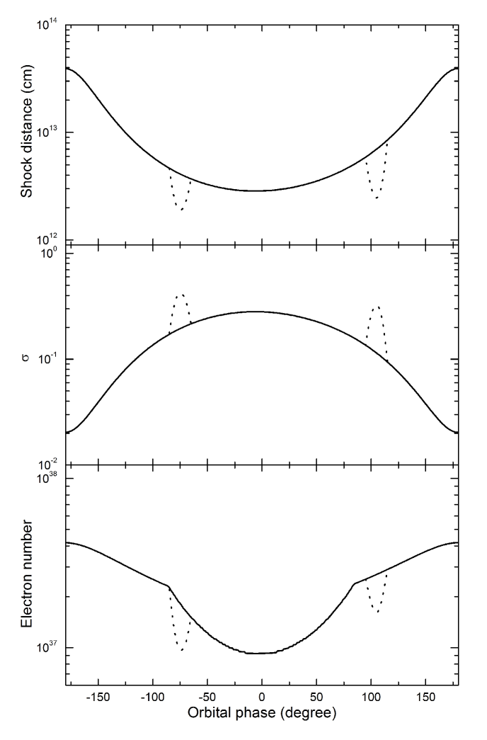
Figure 1: Top panel: The variation of shock distance $r_{\rm s}$ along with the orbital phase; Middle panel: The variation of magnetization parameter $\sigma$ along with the orbital phase; Bottom panel: The variation of electron number $N_{\rm 1-10keV}$ along with the orbital phase. The solid and dotted lines correspond to the conditions without and with the effect of disk respectively.

We will first give some results on the variations of the distance between the shock and the pulsar $r_{\rm s}$, the magnetization parameter $\sigma$ and the electron number $N_{\rm 1-10keV}$ whose typical synchrotron emission frequencies are in the range of 1-10 keV as a function of orbital phase, as shown in Figure 1. The periastron is taken to be at orbital phase $\sim 0\textordmasculine$ throughout the paper. In solid lines, we only consider the polar wind and the input parameters we used are as follows: the terminal velocity of the polar wind $v_{\infty}=1.3\times 10^{8}$ ${\rm cm}$ ${\rm s}^{-1}$, the index of the polar wind $\beta=1.5$, $\dot{M}_{\rm polar}/f_{{\rm w},{\rm polar}}=2\times 10^{-8}$ $M_{\sun}$ ${\rm yr}^{-1}$, the electron distribution index $p=2.2$, the magnetization parameter at light cylinder ($r_{\rm s}=10^{8}{\rm cm}$) $\sigma_{\rm L}=8\times 10^{3}$, the index $\alpha_{\sigma}=1.0$ and $\Gamma_{0}=2\times 10^{5}$. In dotted lines, we add an equatorial component with the initial velocity $v_{\rm 0,disk}=10^{6}$ ${\rm cm}$ ${\rm s}^{-1}$, the index $m=1.5$ and $\dot{M}_{\rm disk}/f_{{\rm w},{\rm disk}}=2\times 10^{-7}$ $M_{\sun}$ ${\rm yr}^{-1}$. In our calculations, the half-opening angle of the disk (projected on the pulsar orbital plane) is $\Delta\theta_{\rm disk}=10\textordmasculine$, and the intersection between the stellar equatorial plane and the orbital plane is inclined at $\theta_{\rm disk}=75\textordmasculine$ to the major axis of the pulsar orbit, which are in the range suggested by Chernyakova et al. (2006) with $\Delta\theta_{\rm disk}\simeq 18\textordmasculine.5$ and $\theta_{\rm disk}\simeq 70\textordmasculine$. These input parameters we used here are chosen by modeling the observations (See below). It can be seen that because the shock distance $r_{\rm s}$ varies along with the orbital phase, the magnetization parameter $\sigma$ and the electron number $N_{\rm 1-10keV}$ evolve accordingly. We can also see from the bottom panel of Figure 1 that because the total electron number evolves as $N_{\rm tot}\propto r_{\rm s}$, $N_{\rm 1-10keV}$ varies as $N_{\rm 1-10keV}\propto r_{\rm s}$ when $r_{\rm s}$ is large. As the pulsar approaching the periastron, the IC process is more and more important and the value of $Y(\gamma_{e,c})$ will increase. At a certain position, some electrons will enter the fast cooling case ($\gamma_{\rm e,c}<\gamma_{\rm e,min}$) with the distribution index being $-(p+1)$ instead of $-p$ in the slow cooling case. At this moment, the electrons will be distributed in a more broad range, and the value of $N_{\rm 1-10keV}$ will decrease more rapidly around the periastron because more and more electrons are cooled to the lower energies. In the dense disk, $r_{\rm s}$ and $\sigma$ reach a minimum and a maximum respectively, and $N_{\rm 1-10keV}$ reaches a minimum because of the smallest electron number and the fastest cooling effect.

3.2 Spectrum

The calculated spectra from $10^{-2}$ eV to 100 TeV are illustrated in Figure 2. The input parameters used here are the same as those in Figure 1. The different types of lines represent the spectra in different orbital phases: the solid line and the dashed line correspond to the conditions at periastron and at the orbital phase of $100\textordmasculine$ respectively, where the effect of the disk is not considered; the dotted line corresponds to the result in the disk (the orbital phase = $-75\textordmasculine$).

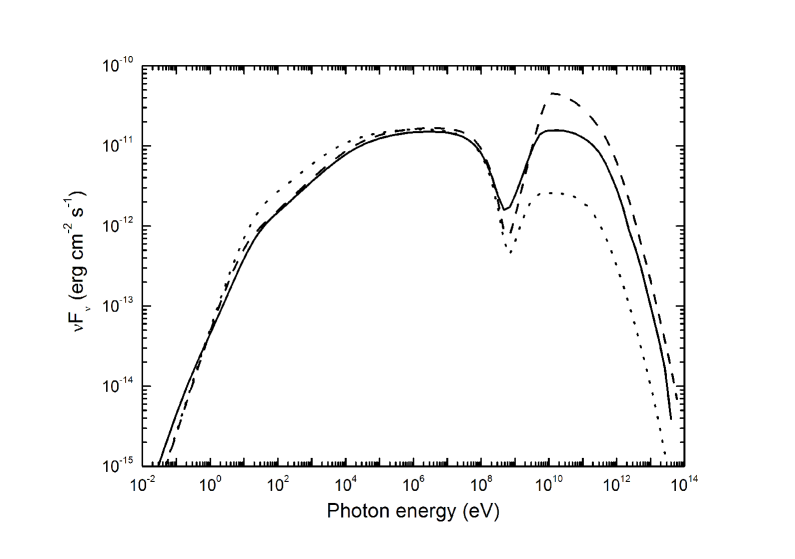
Figure 2: The calculated spectra. The solid line and the dashed line correspond to the conditions at periastron and at the orbital phase of $100\textordmasculine$ respectively, where the effect of disk is not considered; the dotted line corresponds to the result in the disk.

The emission below 100 MeV is mainly from the synchrotron radiation. The shape of synchrotron spectrum is mainly determined by the magnetic field and the electron distribution. It can be seen that between 1-10 keV the flux in the dotted line is the highest in all the three lines. Although the electron number $N_{\rm 1-10keV}$ reaches a minimum in the disk, the radiation flux can be very large because the magnetic field is highest at this moment, as shown in Figure 1. The large flux in the disk will produce an “emission”fa profile in the X-ray light curve. We can also see that in solid line the spectrum below 10 eV is softer and the flux below 1 eV is higher than those in other two lines, which is because more electrons are cooled to this energy range at periastron.

The emission above 1 GeV is mainly produced by the EIC process. The calculated SSC flux is lower than the EIC flux by more than three orders of magnitude for the reason that the SSC emission is strongly suppressed by the KN effect, so we neglect the effect of SSC in our calculations throughout the paper. There are two breaks in the EIC spectra corresponding to the two critical energies $\gamma_{\rm e,min}m_{\rm e}c^{2}$ and $(m_{\rm e}c^{2})^{2}/kT_{\rm eff}$ (Yu 2009). In our calculations, $\gamma_{\rm e,min}m_{\rm e}c^{2}$ corresponds to the first break and $(m_{\rm e}c^{2})^{2}/kT_{\rm eff}\sim$ 0.1 TeV corresponds to the second break in the EIC spectra. We can see that the flux in the dotted line is the lowest in all the three lines. The reasons are as follows: (1) In the disk, the magnetization parameter $\sigma$ gets a maximum and $\gamma_{\rm e,min}$ reaches a minimum accordingly. The small $\gamma_{\rm e,min}$ makes the EIC spectrum begin to break at a low energy; (2) the electron number whose EIC emission frequencies are above 1 GeV decreases duo to the rapid cooling in the disk; (3) The strong wind in the disk pushes the shock to the pulsar, so the photon density from Be star decrease. The low flux in the disk will produce an “absorption” profile in the TeV light curve.

The $Fermi$ Gamma-ray Space Telescope observed the PSR B1259-63/SS 2883 system recently (Tam et al. 2010; Abdo et al. 2010a, 2010b, 2011b; Kong et al. 2011). The Large Area Telescope (LAT) onboard $Fermi$ covers the energy band from 20 MeV to greater than 300 GeV. We can see that in our model, the emission in this energy range is produced by the synchrotron and the EIC processes together (See Section 3.6 for detailed discussion).

3.3 Comparison with observations in the 1-10 keV band

The X-rays from the PSR B1259-63/SS 2883 system was first detected by ROSAT (Cominsky, Roberts & Johnston 1994). After that, the ASCA satellite also observed this system in X-rays (Kaspi et al. 1995; Hirayama et al. 1999). The results from the ASCA satellite show that the X-ray flux from the source is highly variable in different orbital phase, and the light curve has two peaks before and after the periastron respectively. More recently, new X-ray observation data of this source were reported by Chernyakova et al. (2006, 2009). The results include the $XMM-Newton$ observations at the beginning of 2004, some earlier unpublished X-ray data from $BeppoSAX$ and $XMM-Newton$ (Chernyakova et al. 2006), and the unprecedented detailed observations by $Suzaku$, $Swift$, $XMM-Newton$ and $Chandra$ missions during the 2007 periastron passage (Chernyakova et al. 2009). These new data are well in agreement with previous observations, and show that the orbital light curve in X-rays does not exhibit strong orbit-to-orbit variations (Chernyakova et al. 2009).

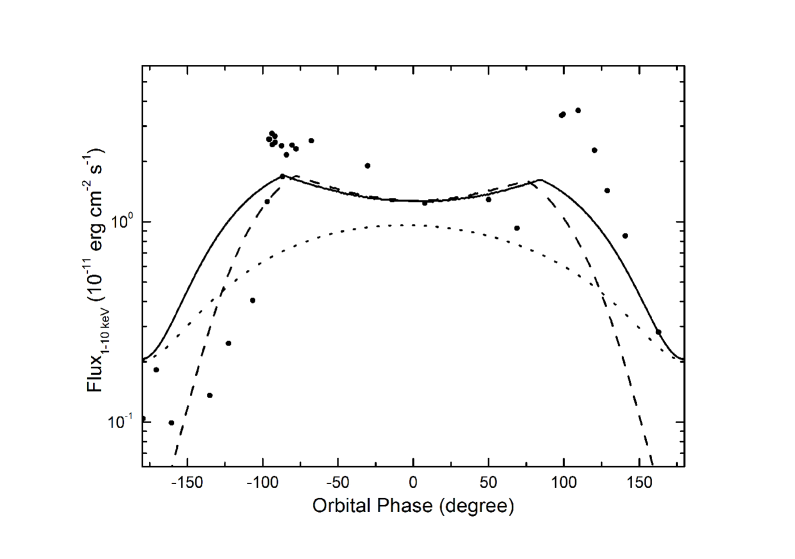
Figure 3: The calculated X-ray light curves and their comparison with observations. The solid line and the dashed line correspond to $\alpha_{\sigma}=1.0$ and $\alpha_{\sigma}=2.0$ respectively. The dotted line corresponds to a constant magnetization parameter $\sigma=0.02$.

Here, we use our model described in Section 2 to reproduce the X-ray light curve of the PSR B1259-63/SS 2883 system. We assume that the X-ray emission is mainly from the synchrotron radiation of the relativistic electrons. The X-ray data are taken from Chernyakova et al. (2006, 2009). In this subsection, we will only use the polar component as the stellar wind. The role of the disk will be discussed later. The calculated light curves and the observed data in 1-10 keV band are presented in Figure 3. Except for special declaration, the parameters we used here are the same as those in the solid lines of Figure 1. In the dotted line, we use a constant value of $\sigma=0.02$ for reference purpose. Differently, in the solid and dashed lines, we make the magnetization parameters vary as $\sigma=\sigma_{\rm L}(r/r_{\rm L})^{-\alpha_{\sigma}}$. We can see that when we use a constant magnetization factor $\sigma=0.02$, as suggested by Tavani & Arons (1997), the resulting light curve cannot explain the two major characteristics in observations: (1) The observed 1-10 keV flux has a sharp rise of about 20 times from apastron to pre-periastron, but the ratio of flux between the maximum and the minimum is only about 5 in the dotted line; (2) In the dotted line, the flux get the maximum at periastron, in opposition to the observations where the flux has a minimum around the periastron. When the variation of $\sigma$ is considered, the calculated results fit the above two characteristics much better. The appearance of this type of bimodal structure is due to the joint action of the variable magnetic field and electron number. As shown in Figure 1, as the pulsar approaching the periastron from the apastron, the magnetization parameter $\sigma$ becomes larger, so the magnetic field $B$ and the synchrotron radiation flux in X-rays ($L_{\rm X}$) should increase more rapidly than those in the situation where $\sigma$ is a constant. A much sharper rise of about 20 times in flux could be produced at this moment. On the other hand, a larger magnetic field $B$ and a smaller shock distance $r_{\rm s}$ around the periastron will make the cooling of particles stronger. Much more electrons will be cooled to the lower energies, and the electron number $N_{1-10\rm keV}$ decreases more rapidly accordingly, as shown in Figure 1. So the flux in the 1-10 keV range has a minimum around the periastron.

The solid and dashed lines in Figure 3 illustrate the effect of the index $\alpha_{\sigma}$ on the 1-10 keV light curves. The parameters used in solid line are the same as those used in the solid line of Figure 1. We choose the value of the magnetization parameter $\sigma$ as a constant at periastron, and take $\alpha_{\sigma}=2.0$ in the dashed line. It is clearly seen that when $\alpha_{\sigma}$ becomes larger, the rise and the drop of flux around the apastron become sharper. This is due to the more rapid change in the value of $\sigma$.

3.4 Comparison with VHE observations above 1 TeV band

As early as 1999, Kirk, Ball & Skjæraasen (1999) predicted that the PSR B1259-63/SS 2883 system could produce VHE radiation, and the light curve should reach the maximum around the periastron. About 5 years later, the TeV $\gamma$-rays from this source were first detected by the High Energy Stereoscopic System (HESS) around its periastron passage in 2004 (Aharonian et al. 2005). This makes the PSR B1259-63/SS 2883 system be the first known binary system to emit photons above 1 TeV (Aharonian et al. 2005). The observed TeV light curve is similar to that in 1-10 keV for having two peaks in pre- and post-periastron respectively with a minimum in flux around the periastron (Aharonian et al. 2005), and is contrary to the prediction by Kirk, Ball & Skjæraasen (1999). The TeV light curve was also found to have significant variations on timescales of days, which makes the system be the first variable VHE source in our Galaxy (Aharonian et al. 2005). The HESS team also observed the source in 2005, 2006 and around the 2007 periastron passage (Aharonian et al. 2009). They found that there is no significant VHE $\gamma$-ray flux near apastron in the 2005 and 2006 observations, and confirmed that this system is a variable TeV emitter.

Here, we use our model introduced in Section 2 to reproduce the TeV light curve of the PSR B1259-63/SS 2883 system. We consider that the photons above 1 TeV are mainly produced by the EIC process. Our modelling light curve are presented in Figure 4 and the parameters used here are the same as those used in Figure 3. The observational TeV data are taken from Aharonian et al. (2005, 2009). We can see that our model can explain the two-peak profile in TeV observations qualitatively.

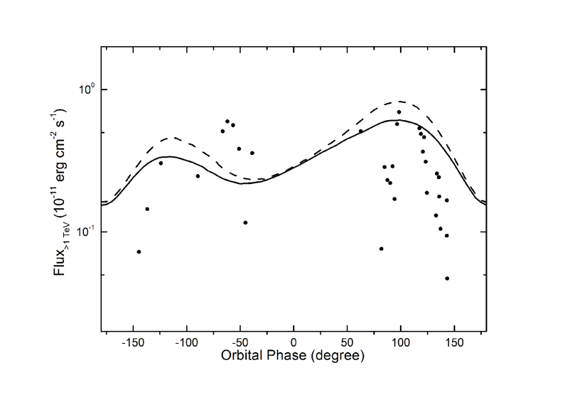
Figure 4: The calculated TeV light curves and their comparison with observations. The solid line and the dashed line correspond to $\alpha_{\sigma}=1.0$ and $\alpha_{\sigma}=2.0$ respectively.

3.5 Effect of the equatorial component in the stellar wind

Be stars like SS 2883 are characterized by strong mass outflows around the equatorial plane. They can produce disks which are slower and denser than the polar wind (Waters et al. 1988). The existence of a disk in the PSR B1259-63/SS 2883 system has been confirmed by the radio observations (Johnston et al. 1996, 2005). The disk of Be star SS 2883 in this binary system is believed to be tilted with respect to the orbital plane. The line of intersection between the disk plane and the orbital plane is oriented at about 90ºwith respect to the major axis of the binary orbit, but the inclination of the disk is not constrained (Wex et al. 1998; Wang, Johnston & Manchester 2004). Chernyakova et al. (2006) analyzed the X-ray light curve of the system detailedly and suggested that the disk has a well-defined Gaussian-profile. The half-opening angle of the disk (projected on the pulsar orbital plane) is $\Delta\theta_{\rm disk}\simeq 18\textordmasculine.5$, and the intersection between the stellar equatorial plane and the orbital plane is inclined at $\theta_{\rm disk}\simeq 70\textordmasculine$ to the major axis of the pulsar orbit.

The presence of disk not only affects the radio radiation from the system, but also plays an important role in producing the X-ray and VHE $\gamma$-ray emission (Chernyakova et al. 2006). Ball et al. (1999) suggested that the acceleration process will be most efficient when the pulsar passes through the disk. Kawachi et al. (2004) suggested that in addition to the relativistic electrons, VHE protons could be produced by the interaction between the pulsar wind and the dense equatorial wind. These hypothesis predict that there will be an increase of flux in disk in both the X-ray and TeV bands and can explain the two-peak profiles in the observed light curves. Recently, Kerschhaggl (2010) found that there is a drop in the TeV light curve when the pulsar passes through the dense disk. They suggested that this is due to an increasing nonradiative cooling effect in the disk.

Here we add the equatorial component of the stellar wind in our calculations, and assume the mass-loss rate and velocity of the equatorial wind have Gaussian profiles to match those of the polar wind. Our results in the X-ray and TeV bands are presented in Figure 5. The solid and dotted lines correspond to the conditions with and without equatorial components respectively. The parameters used here are the same as those used in Figure 1. We can see in Figure 5 that the X-ray flux increases in the passage of disk, but the flux in TeV range decreases significantly at this moment, which is consistent with the analysis by Kerschhaggl (2010). As discussed in Section 3.2, the appearance of an emission component in the X-ray light curve is mainly due to the competition between the decrease of the electron number and the increase of the magnetic field inside the disk, whereas the appearance of an absorption component in the TeV range is due to the low break energy, the decrease of electron number resulting from rapid cooling and the decrease of photon density in the disk.

Figure 5: The effect of disk on the X-ray and TeV light curves. The solid and dotted lines correspond to the conditions with and without the effect of disk respectively.

3.6 Observations by LAT onboard $Fermi$

The PSR B1259-63/SS 2883 system passed through its periastron in mid-December 2010 recently. The LAT onboard $Fermi$ observed this source detailedly. An average flux (above 100 MeV) of $1.2\pm 0.6\times 10^{-7}$ $\rm ph$ $\rm cm^{-2}$ $\rm s^{-1}$ and a photon index of $2.2\pm 0.2$ in the period 2010-11-17 to 2010-12-19 UTC was reported by the $Fermi$ team (Abdo et al. 2010b). They also reported a flux (above 100 MeV) of $1.7\pm 0.4\times 10^{-6}$ $\rm ph$ $\rm cm^{-2}$ $\rm s^{-1}$ with a photon index of $3.0\pm 0.3$ in the period 2011-01-17 to 2011-01-19 UTC, and a flux (above 100 MeV) of $1.8\pm 0.2\times 10^{-6}$ $\rm ph$ $\rm cm^{-2}$ $\rm s^{-1}$ with a photon index of $3.1\pm 0.2$ in the period 2011-01-14 to 2011-01-19 UTC (Abdo et al. 2011b). Some other analyses of LAT data were also done. A flare-like profile with a flux (300 MeV – 100 GeV) of around $4\times 10^{-8}$ $\rm ph$ $\rm cm^{-2}$ $\rm s^{-1}$ and a photon index of about 1.7 in the period 2010-11-18 00:00:00 (UT) to 2010-11-21 00:04:42 (UT) (Tam et al. 2010), and a flux (200 MeV – 100 GeV) of $4.8\pm 0.9\times 10^{-7}$ $\rm ph$ $\rm cm^{-2}$ $\rm s^{-1}$ with a photon index of $3.6\pm 0.4$ in the period 2011-01-14 to 2011-01-16 UTC (Kong et al. 2011) were reported.

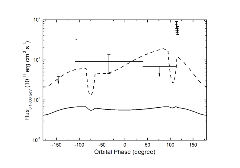
Figure 6: The calculated GeV light curves and their comparison with observations. The emission in solid line is from synchrotron radiation and the emission in dashed line is from the EIC process.

As shown in Figure 2, the emission between 100 MeV and 300 GeV range is produced by the synchrotron and the EIC processes together. In Figure 6, we present our calculated light curve between 100 MeV and 300 GeV using the parameters which are the same as those in the dotted lines of Figure 1. The emission in solid line is from synchrotron radiation and the emission in dashed line is from the EIC process. The observation data are taken from The Astronomer’s Telegrams (ATel; Tam et al. 2010; Abdo et al. 2010a, 2010b, 2011b; Kong et al. 2011), and the flux derived from Tam et al.’s (2010) and Kong et al.’s (2011) reports have been extrapolated to the 100 MeV and 300 GeV energy range using photon indices of 1.7 and 3.6 respectively. We can see that the calculated GeV flux are dominated by the EIC process, but the EIC flux is still lower than the observations. This may be due to two reasons: (1) In the ATel reports, a single power-law has been assumed for the GeV photon spectrum, and we use it to estimate the energy flux in the figure. But in our calculation the spectrum is not a single power-law. It may overestimate the GeV flux by using a single power-law spectrum in the figure. Some recent analyses actually show that the spectrum between 100 MeV and 300 GeV is not a single power-law (Adbo et al. 2011; Tam et al. 2011). (2) Some observations with high flux may be flares, which cannot be produced in the steady model. In other words the flares should be emitting from different region of the shock, which is also suggested by Tam et al. (2011) comparing the 100 MeV to 300 GeV spectra with the $>$ 300 GeV gamma-ray spectra. We suggest that the flares may come from the relativistic Doppler-boosting effect (Dubus, Cerutti & Henri 2010). Bogovalov et al. (2008) presented a hydrodynamic simulation of the interaction between relativistic and nonrelativistic wind in PSR B1259-63/SS 2883 system. They found that the electrons in the shocked pulsar wind can be accelerated from bulk Lorentz factors $\sim 1$ around the termination shock to nearly 100 far away. The spectrum of synchrotron emission in our calculations peaks at about 0.1 GeV. With such a large bulk Lorentz factor of $\sim$ 100, the peak will be Doppler-boosted to about 10 GeV, which could be detected by $Fermi$ satellite. However, emission from the electrons with a bulk Lorentz factor of 100 should be strongly beamed. When the line-of-sight is in the beaming direction, we can receive the GeV flux, otherwise, the GeV photons disappear. In this case, a flare profile may be found. The much higher intensity of the flares is mainly due to the beaming effect because instead of radiating isotropically the GeV photons from the large bulk Lorentz factor region is highly beamed at a much smaller solid angle. If the geometry of the shock has a simple bow shock structure at the tail, we expect that two flares will occur when the line of sight passes through the two edges of the cone of the bow shock and each flare can last about an orbital phase $2/\Gamma\sim 12^{\circ}(\Gamma/10)^{-1}$, where $\Gamma$ is the bulk Lorentz factor at the tail of the shock. If the photon numbers are sufficiently high during the flares we should be able to find the synchrotron cut-off energy ($E_{\rm syn}\sim 100$ MeV cf. Figure 2) boosting to $\Gamma E_{\rm syn}\sim 1$ GeV $(\Gamma/10)$ in these flares and the general spectrum in $Fermi$ range should satisfy a simple power with exponential cut-off.

Recently, Tam et al. (2011) found the flux in the flaring period in Fermi observations is enhanced by a factor of 5-10, which suggests a Doppler factor of around 1.5-2. With a low energy break around 10 keV observed by $Suzaku$ (Uchiyama et al. 2009), the enhancement has a factor of only about 3 in the X-ray band, which is smaller than that in the GeV band and is less obvious. In addition, the flaring period is near the second peak in the X-ray light curve. This peak may be produced by the effect of Doppler boosting and disk together. For the TeV flux, because more IC scattering occur in the KN regime for $\Gamma>1$, the TeV flux should be suppressed. In addition, the stellar photon density in the bow shock tail is smaller than that in the shock apex, so the IC emission should be lower accordingly. The increase of TeV flux due to the Doppler boosting and the decrease due to the KN effect and smaller photon density will compensate each other, and the Doppler boosting may not modulate the TeV light curve significantly. Furthermore, because the emission from the shock tail is temporally and spectrally different with that from the shock apex, the magnetic fields and the electron distributions may not be the same in these two ranges.

4 Conclusion and Discussion

The PSR B1259-63/SS 2883 system is an attractive binary system, and is also an unique astrophysical laboratory for probing the time dependent interaction between the pulsar wind and stellar wind, and studying the physics of the pulsar wind in a different range compared with an isolated pulsar. In this paper, we have modeled the X-ray and TeV observations of the source using the wind interaction model under the hypothesis that the X-ray emission is mainly from the synchrotron process and the TeV photons are mainly produced by the EIC effect where the relativistic electrons in the shock up-scatter the photons from the Be star. The effect of the disk exhibits an emission and an absorption components in the X-ray and TeV bands respectively. More importantly, we assume that the microphysics parameters are not constant and take the magnetic parameter $\sigma$ varying as a power-law form along with the distance between the termination shock and the pulsar. This is a reasonable assumption because $\sigma$ has a very large value at the light cylinder and reaches a very small value of about 0.003 at a distance of about 0.1 pc from the pulsar (Kennel & Coroniti 1984a, 1984b). The variation of microphysics parameters has also been suggested in some other astrophysical phenomena like Gamma-ray bursts (Kong et al. 2010). We also try to explain the GeV light curve which is observed by LAT very recently, and suggest that the actual photon spectra may not be power-law distributed as reported in the ATel and some flare-like profile may come from the relativistic Doppler-boosting effect.

In a recent paper, van Soelen & Meintjes (2011) investigated the effect of the infrare emission from the Be star’s disk on the inverse Compton process. The free-free and free-bound emission occurred in the disk is thought to produce an infrared excess in the Be star’s photon spectrum. The scattering of this infrared excess will influence the gamma-ray production. As discussed by van Soelen & Meintjes (2011), for the electrons with Lorentz factors $\gamma_{\rm e}>10^{5}$, the scattering of photons around the peak in the stellar spectrum will be in the KN limit, while the scattering with photons in the infrared excess will be in the Thompson limit and increase the emission at GeV band. But for the broad electron distribution with $\gamma_{\rm e,min}\sim 10^{4}$, the scattering with photons around the peak of the stellar spectrum will occur in the Thompson limit, and most of the GeV photons are produced by the Thompson scattering of the whole stellar spectrum. So the effect of the infrared excess on the spectrum could be negligible. In our calculations above, the electron distributions are very broad with ${\rm min}(\gamma_{\rm e,min},\gamma_{\rm e,c})$ between a few $\times 10^{3}$ to a few $\times 10^{4}$. The resulting influence on the GeV flux by the infrared excess is insignificant, so we do not consider this effect in our calculations.

There are also some other binary systems in our Galaxy similar to PSR B1259-63/SS 2883 being found for emitting the X-ray and VHE emission, such as LS 5039 (Aharonian et al. 2006), LS I+61º303 (Albert et al. 2006) and possibly HESS J0632+057 (Hinton et al. 2009). Our model can possibly be used in explaining the broadband observational light curves in these systems. However, the orbital properties are different in these systems. In PSR B1259-63/SS 2883, the separation between the pulsar and the massive star is 0.7-10 AU. But the separation is only about 0.1-0.2 AU in LS 5039 and 0.1-0.7 AU in LS I+61º303 (Dubus 2006). The magnetization parameter $\sigma$ should be larger accordingly. The detailed study of the radiation from the LS 5039 and the LS I+61º303 systems could help us to understand the physical condition of the pulsar wind in the position where is much closer to pulsar compared with the PSR B1259-63/SS 2883 system.

References

- (1) Abdo, A. A., Ackermann, M., Ajello, M., et al. 2011a, ATeL, 3054
- (2) Abdo, A. A., Grove, J. E., Dubois, R., et al. 2010a, ATeL, 3054
- (3) Abdo, A. A., Parent, D., Grove, J. E., et al. 2010b, ATeL, 3085
- (4) Abdo, A. A., Parent, D., Dubois, R., et al. 2011b, arXiv:1103.4108
- (5) Aharonian, F., Akhperjanian, A. G., Anton, G., et al. 2009, A&A, 507, 389
- (6) Aharonian, F., Akhperjanian, A. G., Aye, K. M., et al. 2005, A&A, 442, 1
- (7) Aharonian, F., Akhperjanian, A. G., Bazer-Bachi, A. R., et al. 2006, A&A, 460, 743
- (8) Aharonian, F. A., & Atoyan A. M. 1981, Ap&SS, 79, 321
- (9) Albert, J., Aliu, E., Anderhub, H., et al. 2006, Science, 312, 1771
- (10) Ball, L, & Kirk, J. G. 2000, Astropart. Phys., 12, 335
- (11) Ball, L, Melatos, A., Johnston, S., & Skjæraasen, O. 1999, ApJL, 514, L39
- (12) Blumenthal G. R., & Gould R. J. 1970, Rev. Mod. Phys., 42, 237
- (13) Bogovalov, S. V., Khangulyan, D. V., Koldoba, A. V., et al. 2008, MNRAS, 387, 63
- (14) Cheng, K. S., Ho, C., & Ruderman, M. 1986a, ApJ, 300, 500
- (15) Cheng, K. S., Ho, C., & Ruderman, M. 1986b, ApJ, 300, 522
- (16) Chernyakova, M., Neronov, A., Aharonian, F., et al. 2009, MNRAS, 397, 2123
- (17) Chernyakova, M., Neronov, A., Lutovinov, A., et al. 2006, MNRAS, 367, 1201
- (18) Cominsky, L., Roberts, M., & Johnston, S. 1994, ApJ, 427, 978
- (19) Dubus, G., 2006, A&A, 456, 801
- (20) Dubus, G., Gerutti, B., & Henri, G. 2010, A&A, 516, id.A18
- (21) Ginzburg, V. L., & Syrovatskii, S. I. 1964, The Origin of Cosmic Rays (Macmillan)
- (22) Gould, R. G., & Schréder, G. P. 1967, Phys. Rev., 155, 1404
- (23) He, H. N., Wang, X. Y., Yu, Y. W., & Mészáros, P. 2009, ApJ, 706, 1152
- (24) Hinton, J. A., Skilton, J. L., Funk, S., et al. 2009, ApJL, 690, L101
- (25) Hirayama, M., Cominsky, L. R., Kaspi, V. M., et al. 1999, ApJ, 521, 718
- (26) Johnston, S., Ball, L., Wang, N., & Manchester, R. N. 2005, MNRAS, 358, 1069
- (27) Johnston, S., Manchester, R. N., Lyne, A. G., et al., 1992, ApJL, 387, L37
- (28) Johnston, S., Manchester, R. N., Lyne, A. G., et al., 1994, MNRAS, 268, 430
- (29) Johnston, S., Manchester, R. N., Lyne, A. G., et al., 1996, MNRAS, 279, 1026
- (30) Kaspi, V. M., Tavani, M., Nagase, F., et al. 1995, ApJ, 453, 424
- (31) Kawachi, A., Naito, T., Patterson, J. R., et al. 2004, ApJ, 607, 949
- (32) Kennel, C. F., & Coroniti, F. V. 1984a, ApJ, 283, 694
- (33) Kennel, C. F., & Coroniti, F. V. 1984b, ApJ, 283, 710
- (34) Kerschhaggl, M. 2010, A&A, 525, id.A80
- (35) Khangulyan, D., Hnatic, S., Aharonian, F., & Bogovalov, S. 2007, MNRAS, 380, 320
- (36) Kirk, J. G., Ball, L., & Skjæraasen, O. 1999, Astropart. Phys., 10, 31
- (37) Kong, A. K. H., Huang, R. H. H., Tam, P. H. T., & Hui, C. Y., 2011, ATeL, 3111
- (38) Kong, S. W., Wong, A. Y. L., Huang, Y. F., & Cheng, K. S. 2010, MNRAS, 402, 409
- (39) Neronov, A., & Chernyakova, M. 2007, Ap&SS, 309, 253
- (40) Rybicki, G. B., & Lightman, A. P. 1979, Radiative Processes in Astrophysics (New York: Wiley)
- (41) Sari, R., & Esin, A. A. 2001, ApJ, 548, 787
- (42) Sari, R., Piran, T., & Narayan, R. 1998, ApJL, 497, L17
- (43) Takata, J., & Taam, R. E. 2009, ApJ, 702, 100
- (44) Takata, J., Wang, Y., & Cheng, K. S. 2010, ApJ, 715, 1318
- (45) Tam, P. H. T., Kong, A. K. H., Huang, R. H. H., & Hui, C. Y., 2010, ATeL, 3046
- (46) Tam, P. H. T., Huang, R. H. H., Takata, J., et al. 2011, ApJL, submitted
- (47) Tavani, M., & Arons, J. 1997, ApJ, 477, 439
- (48) Uchiyama, Y., Tanaka, T., Takahashi, T., et al. 2009, ApJ, 698, 911
- (49) van Soelen, B., & Meintjes, P. J. 2011, MNRAS, 412, 1721
- (50) Wang, N., Johnston, S., & Manchester, R. N. 2004, MNRAS, 351, 599
- (51) Wang, X. Y., He, H. N., Li, Z. et al. 2010, ApJ, 712, 1232
- (52) Waters, L. B. F. M., Taylor, A. R., van den Heuvel, E. P. J., et al. 1988, A&A, 198, 200
- (53) Wex, N, Johnston, S., Manchester, R. N., et al. 1998, MNRAS, 298, 997
- (54) Yu, Y. W. 2009, PhD thesis, Huazhong Normal University
- (55) Zabalza, V., Paredes, J. M., & Bosch-Ramon, V. 2011, A&A, 527, id.A9
- (56) Zhang, L., & Cheng, K. S. 1997, ApJ, 487, 370