Cosmic Evolution in Brans-Dicke Chameleon Cosmology

Abstract

Abstract: We have investigated the Brans-Dicke Chameleon theory of gravity and obtained exact solutions of the scale factor $a(t)$, scalar field $\phi(t)$, an arbitrary function $f(\phi)$ which interact with the matter Lagrangian in the action of the Brans-Dicke Chameleon theory and potential $V(\phi)$ for different epochs of the cosmic evolution. We plot the functions $a(t)$, $\phi(t)$, $f(t)$ and $V(\phi)$ for different values of the Brans-Dicke parameter. In our models, there is no accelerating solution, only decelerating one with $q>0$. The physical cosmological distances have been investigated carefully. Further the statefinder parameters pair and deceleration parameter are discussed.

I Introduction

The Brans-Dicke (BD) theory of gravity defined by a scalar field $\phi$ and a constant coupling function $\omega$ BD1 , is perhaps the most natural extension of general relativity (GR) which is obtained in the limit of $\omega\rightarrow\infty$ and $\phi$= constant KN ; JDB ; JMA . An imperative property of the BD theory of gravity is that it yields simple expanding solutions CM for scalar field $\phi(t)$ and scale factor $a(t)$ which are well-matched with solar system experiments PMG ; SP ; AGR . There are many works on interesting physical aspects of the BD theorysergei .

In a recent paper the dynamics of the cosmic evolution has been investigated in the formalism of generalized BD theory of gravity (where $\omega$ is not a constant but a function of $\phi(t)$) singh . There a consistent solution of the generalized BD equations of motion based on simple power-law temporal behavior of $a$, $\phi$ and $\omega$ is obtained.

In the present paper, a BD theory in which there is a non-minimal coupling between the scalar field and the matter field is considered. Thereby the action and the field equations are modified due to the coupling of the scalar field with the matter. In the literature such type of scalar field usually called chameleon field JK .We note that a chameleon field requires an strict form of its potential in order to avoid the appearance of fifth forces or violations of the Equivalence Principle, so that a chameleon model has to present a realistic potential. This is due to the fact that the physical properties of the scalar field, such as its mass, depend delicately on the environment. Moreover, in high density regions, the chameleon mix together with its environment and becomes essentially invisible to searches for Equivalence Principle violation and fifth force JK . Further more, it was shown that in the presence of chameleon field, all existing constraints from planetary orbits, such as those from lunar laser ranging are easily satisfied JK ; TP . The explanation is that the chameleon-mediated force between two large objects, such as the Earth and the Sun, is much weaker than one would bluntly expect. In particular, it was shown that the deviations from Newtonian gravity due to the chameleon field of the Earth are suppressed by nine orders of magnitude by the thin-shell effect TP . Some other studies on the chameleon gravity have been investigated in PB ; SSG ; KK .

Our work differs from that of Ref. singh in that we assume a non-minimal coupling between the scalar field and the matter field. besides, we are taking $\omega$ as a constant and not a function of $\phi(t)$. Our aim is to investigate the dynamics of the potential $V(\phi)$ and the function $f(\phi)$ (these are defined in the next section) alongside the scale factor $a(t)$ and the scalar field $\phi(t)$. In other words we are interested to find exact solutions of $a(t)$, $\phi(t)$, $f(\phi)$ and $V(\phi)$ for different epochs of the cosmic evolution. The stability analysis of the solutions is important. But it will be beyond the scope of our paper. Such analysis can be done using the similar methodology, as it has been done in stability1 , by defining dimensionless variables. The stability of BD with Chameleon field has been done already in stability2 for the same system of equations as we have.

The statefinder parameters pair $\{r,s\}$, allows one to explore the properties of dark energy (DE) independent of the model sahni . It has been used to distinguish flat models of the DE. Recently this pair has been evaluated for different models Zh1 ; We ; Zh2 ; Hu ; Zha ; HuM ; Zim ; Sho ; JD ; SJ ; Mde ; Sharif . In the framework of Brans-Dicke Chameleon cosmology, the statefinder parameters are studied in sr .

Plan of the paper is as follows. In the next section we give the basic equations of cosmic evolution with chameleon scalar field. In the section III we discuss our model and obtain exact solution of $a(t)$, $\phi(t)$, $f(\phi)$ and $V(\phi)$ for (A) radiation dominated era, (B) dust fluid era and (C) vacuum energy dominated era. In the section IV the statefinder parameters and the deceleration parameter are investigated. The cosmological distances have been discussed in section V. Finally we conclude our discussion in section VI.

II Cosmic evolution with Chameleon scalar field

We begin with the BD chameleon theory in which the scalar field is coupled non-minimally to the matter field via the action jamil

$$S=\int{d^{4}x\sqrt{-g}\left(\phi{R}-\frac{\omega}{\phi}g^{\mu\nu}\partial_{\mu}\phi\partial_{\nu}\phi-V(\phi)+f(\phi)L_{m}\right)},$$ (1)

where ${R}$ is the Ricci scalar curvature, $\phi$ is the BD scalar field with a potential $V(\phi)$. The chameleon field $\phi$ is non-minimally coupled to gravity, $\omega$ is the dimensionless BD parameter. The last term in the action indicates the interaction between the matter Lagrangian $L_{m}$ and some arbitrary function $f(\phi)$ of the BD scalar field. In the limiting case $f(\phi)=1$, we obtain the standard BD theory.

The gravitational field equations derived from the action (1) with respect to the metric is

$$R_{\mu\nu}-\frac{1}{2}g_{\mu\nu}R = \frac{f(\phi)}{\phi}T_{\mu\nu}+\frac{\omega}{\phi^{2}}\Big{(}\phi_{\mu}\phi_{\nu}-\frac{1}{2}g_{\mu\nu}\phi^{\alpha}\phi_{\alpha}\Big{)}$$ (2)

$$+\frac{1}{\phi}[\phi_{\mu;\nu}-g_{\mu\nu}\Box\phi]-g_{\mu\nu}\frac{V(\phi)}{2\phi}.$$

where $T_{\mu\nu}$ represents the stress-energy tensor for the fluid filling the spacetime which is represented by the perfect fluid

$$T_{\mu\nu}=(\rho+p)u_{\mu}u_{\nu}+pg_{\mu\nu},$$ (3)

where $\rho$ and $p$ are the energy density and pressure of the perfect fluid which we assume to be a mixture of different kinds of matters. Actually there is only chameleon field, whose pressure and density are given by a perfect fluid stress tensor. For different state parameters, this fluid behaves differently, like matter, radiation or DE. Also $u^{\mu}$ is the four-vector velocity of the fluid satisfying $u^{\mu}u_{\mu}=-1$. The Klein-Gordon equation (or the wave equation) for the scalar field is

$$\Box\phi=\frac{T}{2\omega+3}\Big{(}f-\frac{1}{2}\phi f_{,\phi}\Big{)}+\frac{1}{2\omega+3}(\phi V_{,\phi}-2V),$$ (4)

where $T$ is the trace of (3)and $\Box=\nabla^{\mu}\nabla_{\mu}$ in which the operator $\nabla_{\mu}$ represents covariant derivative. The homogeneous and isotropic Friedmann-Robertson-Walker (FRW) universe is described by the metric

$$ds^{2}=-dt^{2}+a^{2}(t)\left(\frac{dr^{2}}{1-kr^{2}}+r^{2}d\Omega^{2}\right),$$ (5)

where $a(t)$ is the scale factor, and $k=-1,0,+1$ corresponds to open, flat, and closed universes, respectively. Variation of action (1) with respect to metric (5) for a flat $k=0$ universe filled with perfect fluid yields the following field equations

$$H^{2}-\frac{\omega}{6}\frac{\dot{\phi}^{2}}{\phi^{2}}+H\frac{\dot{\phi}}{\phi}=\frac{f(\phi)}{3\phi}\rho{+\frac{V(\phi)}{6\phi}},$$ (6)

$$2\frac{{\ddot{a}}}{a}+H^{2}+\frac{\omega}{2}\frac{\dot{\phi}^{2}}{\phi^{2}}+2H\frac{\dot{\phi}}{\phi}+\frac{\ddot{\phi}}{\phi}=-\frac{p}{\phi}{+\frac{V(\phi)}{2\phi}},$$ (7)

where $H=\dot{a}/a$ is the Hubble parameter. Here, a dot indicates differentiation with respect to the cosmic time $t$. The dynamical equation (energy conservation) for the scalar field is

$$\ddot{\phi}+3H\dot{\phi}-\frac{\rho-3p}{2\omega+3}\Big{(}f-\frac{1}{2}\phi f_{,\phi}\Big{)}+\frac{2}{2\omega+3}\Big{(}V-\frac{1}{2}\phi V_{,\phi}\Big{)}=0.$$ (8)

Similarly the energy conservation for the cosmic fluid is

$$\dot{\rho}+3H(\rho+p)=0.$$ (9)

We shall use the equation of state (EoS) for the fluid $p=\gamma\rho$, thus (9) yields

$$\rho=Ca^{-3(1+\gamma)}.$$ (10)

III Our model

Observational data of SN Ia suggests that theoretical models based on power-law forms of the Chameleon potential $V(\phi)$ and scalar function $f(\phi)$ are consistent with the data sr . Hence we shall follow the procedure of singh and will obtain solution of the above dynamical equations (6) to (9), by assuming power law dependence on time for $a(t)$, $\phi(t)$, $f(\phi)$ and $V(\phi)$.

$$a(t)=a_{0}\Big{(}\frac{t}{t_{0}}\Big{)}^{\alpha},$$ (11)

$$\phi(t)=\phi_{0}\Big{(}\frac{t}{t_{0}}\Big{)}^{\beta},$$ (12)

$$f(\phi(t))\sim\phi(t)^{n}=f_{0}\Big{(}\frac{t}{t_{0}}\Big{)}^{n\beta},$$ (13)

$$V(\phi(t))\sim\phi(t)^{m}=V_{0}\Big{(}\frac{t}{t_{0}}\Big{)}^{m\beta}.$$ (14)

Note that $\omega$ is a constant BD parameter and $a_{0}$, $\phi_{0}$, $f_{0}$ and $V_{0}$ are also constants. Also notice that dynamical system is a closed system i.e. four differential equations (6) to (9) for four unknown parameters ($\alpha$, $\beta$, $m$, $n$) to be determined. $\alpha$ must be positive for an expanding Universe while other parameters are free. Using (11) in (10), we get

$$\rho=\rho_{0}\Big{(}\frac{t}{t_{0}}\Big{)}^{-3\alpha(1+\gamma)},\ \ \ p=\gamma\rho_{0}\Big{(}\frac{t}{t_{0}}\Big{)}^{-3\alpha(1+\gamma)}.$$ (15)

Using the set of ansatz functions(11-15) we get,

$$\alpha^{2}-\frac{\omega}{6}\beta^{2}+\alpha\beta=0,$$ (16)

$$f_{0}\rho_{0}=-\frac{V_{0}}{2},$$ (17)

$$(n-m)\beta=3\alpha(1+\gamma).$$ (18)

We now proceed to check the consistency of above equations with Eq.(8) which is the wave equation for the scalar field $\phi(t)$. Using eqs. (11-15) Eq.(8) reduces to

$$\beta(\beta-1+3\alpha)=0,$$ (19)

$$(2-m)V_{0}=\rho_{0}f_{0}(2-n)(1-3\gamma),$$ (20)

$$(m-n)\beta=-3\alpha(1+\gamma).$$ (21)

The above Eq. (19) implies that we can have $\beta=0$ or $\beta=1-3\alpha$. The first one results that

$$\phi(t)=\phi_{0},$$ (22)

$$f(\phi)=f_{0},$$ (23)

$$V(\phi)=V_{0}.$$ (24)

The above set of functions or their equivalent value $\beta=0$ in (16) gives us $\alpha=0$. But we remove $\beta=0$ in our toy model we must take $\alpha>0$. Thus in the present work we discard this special case and limit ourselves only to

$$\beta=1-3\alpha$$ (25)

Now we analyze different cosmological epochs. That is the cases of $\gamma=\frac{1}{3}$, $\gamma=0$. We remove completely the case with $\gamma=-1$, since as we pointed it previously , in our models, there is no accelerating solution, only decelerating one with $q>0$.

III.1 Radiation dominated ($\gamma=1/3$)

In this case Eq. (20)gives $m=2$. Substituting $\beta=1-3\alpha$ in (16) we obtain

$$\alpha=\frac{3(\omega+1)\pm\sqrt{6\omega+9}}{12+9\omega},$$ (26)

$$\beta=\frac{1\mp\sqrt{6\omega+9}}{4+3\omega}.$$ (27)

Now from (18) we obtain

$$n=\frac{14+12\omega\pm 2\sqrt{6\omega+9}}{1\mp\sqrt{6\omega+9}}$$ (28)

Thus we have

$$a(t)=a_{0}\Big{(}\frac{t}{t_{0}}\Big{)}^{\frac{3(\omega+1)\pm\sqrt{6\omega+9}}{12+9\omega}},$$ (29)

$$\phi(t)=\phi_{0}\Big{(}\frac{t}{t_{0}}\Big{)}^{\frac{1\mp\sqrt{6\omega+9}}{4+3\omega}},$$ (30)

$$f(\phi(t))=f_{0}\Big{(}\frac{t}{t_{0}}\Big{)}^{\frac{14+12\omega\pm 2\sqrt{6\omega+9}}{4+3\omega}},$$ (31)

$$V(\phi(t))=V_{0}\Big{(}\frac{t}{t_{0}}\Big{)}^{2\frac{1\mp\sqrt{6\omega+9}}{4+3\omega}}.$$ (32)

Below we plot some figures include the time behavior of the set of functions $a(t)$, $\phi(t)$, $f(\phi(t))$, $V(\phi(t))$ for some large values of the parameter $\omega$. The first two figures show the accelerated expansion of Universe for some large values of the BD parameter.

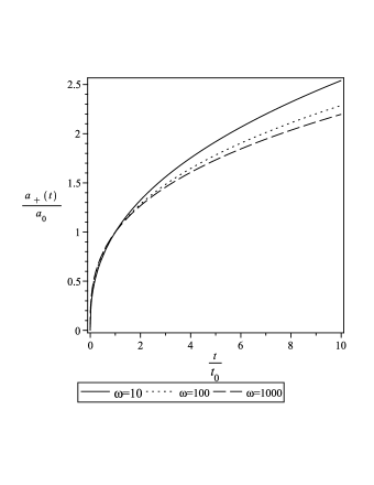
Figure 1: Variation of scale factor $\frac{a_{+}(t)}{a_{0}}$ for different values of the BD parameter $\omega$.

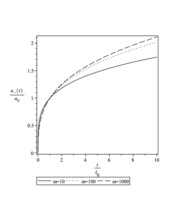
Figure 2: Variation of scale factor $\frac{a_{-}(t)}{a_{0}}$ for different values of the BD parameter $\omega$.

The next two figure show the two possible values of the scalar field for a sample of large BD parameter.

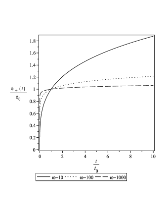
Figure 3: Variation of the one possible value of the scalar field for a sample of large BD parameter $\omega$.

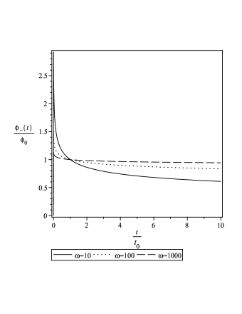
Figure 4: Variation of the another possible value of the scalar field for a sample of large BD parameter $\omega$.

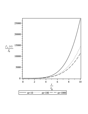
Figure 5: Variation of $f_{+}(t)$ for a sample of large BD parameter $\omega$.

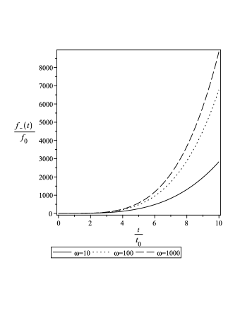
Figure 6: Variation of $f_{-}(t)$ for a sample of large BD parameter $\omega$.

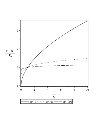
Figure 7: Variation of $V_{+}(t)$ for a sample of large BD parameter $\omega$.

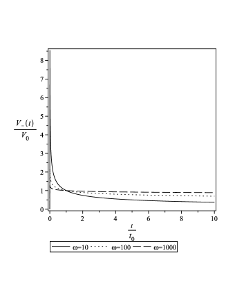
Figure 8: Variation of $V_{-}(t)$ for a sample of large BD parameter $\omega$.

We obtain that the radiation dominant toy model is a simple square power model. Here we plot the potential function as a function of the scalar field for some values of the $\phi_{0},V_{0}$.

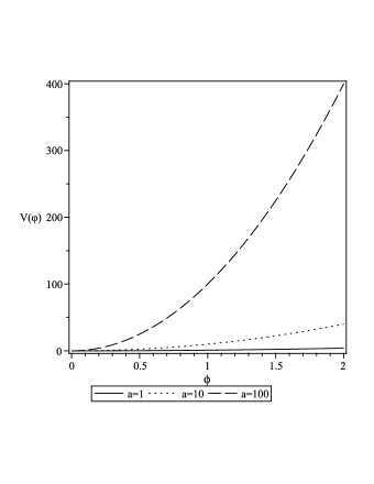
Figure 9: Variation of $V(\phi)$ for a sample of the parameter $a=\frac{V_{0}}{(\phi_{0})^{2}}$.

Remind that for the limit of the very large BD parameter $\omega$ which we expect that the theory must has a GR limit , the exponents and the functions are

$$\alpha_{GR}(t)=\frac{1}{3}$$ (33)

$$\beta\simeq 0,$$ (34)

$$n\simeq 0.$$ (35)

$$a_{GR}(t)=a_{0}\Big{(}\frac{t}{t_{0}}\Big{)}^{\frac{1}{3}}$$ (36)

$$\phi(t)\simeq\phi_{0},$$ (37)

$$f(\phi(t))\simeq f_{0},$$ (38)

$$V(\phi(t))\simeq V_{0}.$$ (39)

The plot of the scale factor for the GR limit is Fig.(10)

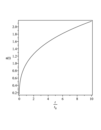
Figure 10: Variation of scale factor in GR limit

III.2 Dust fluid ($\gamma=0$)

This case from (20,21) we’ve

$$m+\frac{n}{2}=3$$ (40)

$$(m-n)=-\frac{9(\omega+1)\pm 3\sqrt{6\omega+9}}{1\mp\sqrt{6\omega+9}}$$ (41)

from (40,41) we obtain

$$n=\frac{2(3\omega+4)}{1\mp\sqrt{6\omega+9}}$$ (42)

$$m=\frac{-(1+3\omega)\mp 3\sqrt{6\omega+9}}{1\mp\sqrt{6\omega+9}}$$ (43)

Thus we have

$$f(\phi(t))=f_{0}\Big{(}\frac{t}{t_{0}}\Big{)}^{2}$$ (44)

$$V(\phi(t))=V_{0}\Big{(}\frac{t}{t_{0}}\Big{)}^{\frac{-(1+3\omega)\mp 3\sqrt{6\omega+9}}{4+3\omega}}.$$ (45)

for large values of the BD parameter $\gamma$, we have $V(\phi(t))=V_{0}\Big{(}\frac{t}{t_{0}}\Big{)}^{-1}$.

IV Statefinder parameters and deceleration parameter

The statefinder parameters $r$ and $s$ depends on the third and second derivatives of the scale factor $a$, just as the dependence of the Hubble parameter $H$ and the deceleration parameter $q$ on its first and second derivatives respectively.

The deceleration parameter is defined as

$$q=-\frac{\ddot{a}}{a\dot{a}^{2}}.$$ (46)

The statefinder parameters are sahni

$$r=\frac{\dddot{a}a^{2}}{\dot{a}^{3}},\ \ s=\frac{r-1}{3(q-\frac{1}{2})}.$$ (47)

For Eq. (29), the above three parameters take the form

$$q_{\pm} = \frac{3+2\omega\mp\sqrt{9+6\omega}}{\omega},$$

$$r_{\pm} = \frac{(\mp 21\mp 15\omega+\sqrt{9+6\omega})(\mp 9\mp 6\omega+\sqrt{9+6\omega})}{(3+3\omega+\sqrt{9+6\omega})^{2}},$$

$$s_{\pm} = \frac{6+6\omega\mp\sqrt{9+6\omega}}{3\omega}.$$ (48)

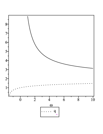
Figure 11: Variation of the deceleration parameter $q_{+,-}$. The line is $q_{+}$ and dot denotes $q_{-}$.

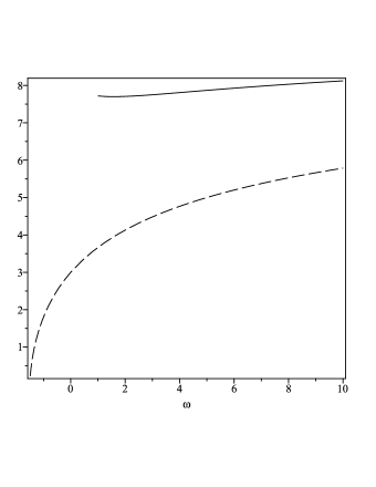
Figure 12: Variation of the parameter $r_{+,-}$. The line is $r_{+}$ and dash denotes $r_{-}$.

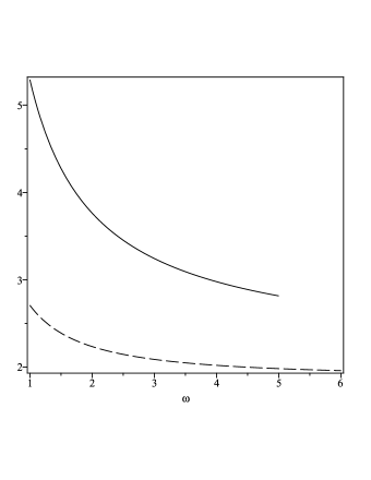
Figure 13: Variation of the parameter $s_{+,-}$. The line is $s_{+}$ and dash denotes $s_{-}$.

V Cosmological distances

In this section we discuss the time dependent cosmological distances of the models presented in sections A,B.

V.1 Lookback time

If a photon is emitted by a source at the instant $t$ and received at time $t_{0}$, then the photon travel time or the lookback time $t-t_{0}$ is defined by

$$t-t_{0}=-\int_{0}^{z}\frac{dz}{H(z)(1+z)},$$ (49)

where $a_{0}$ is the present value of the scale factor of the Universe. If a photon emitted by a source and received by an observer at time $t_{0}$ then the proper distance between them is defined by

$$t-t_{0}=(1+z)^{-\frac{1}{\alpha}}.$$ (50)

The Figure-14 shows the behavior of the lookback time as a function of the redshift for value different values of the $\omega$ and for the plus sign in (26).

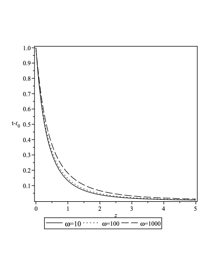
Figure 14: The behavior of the lookback time as a function of the redshift for values $\omega$.

V.2 Proper distance

If a photon emitted by a source and received by an observer at time $t_{0}$ then the proper distance between them is defined by

$$d=a_{0}\int_{a}^{a_{0}}\frac{da}{aH^{2}}=\int_{0}^{z}\frac{dz}{H^{2}(z)(1+z)},$$ (51)

which for (29) simplifies to

$$d=\frac{1}{2\alpha}(1-\frac{1}{(1+z)^{\frac{2}{\alpha}}}).$$ (52)

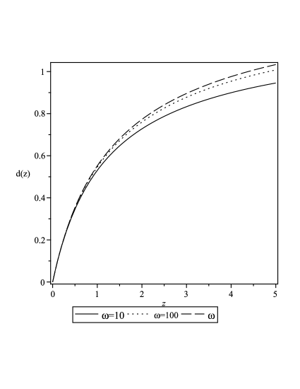
Figure 15: The behavior of the proper distance as a function of the redshift for values $\omega$.

V.3 Luminosity distance

If $L$ be the total energy emitted by the source per unit time and $\ell$ be the apparent luminosity of the object then the luminosity distance $d_{L}=\left(\frac{L}{4\pi\ell}\right)^{\frac{1}{2}}$ evolves as

$$d_{L}=d(1+z).$$ (53)

The figure (16) shows the variation of the luminosity distance as a function of the exponent $\omega$.

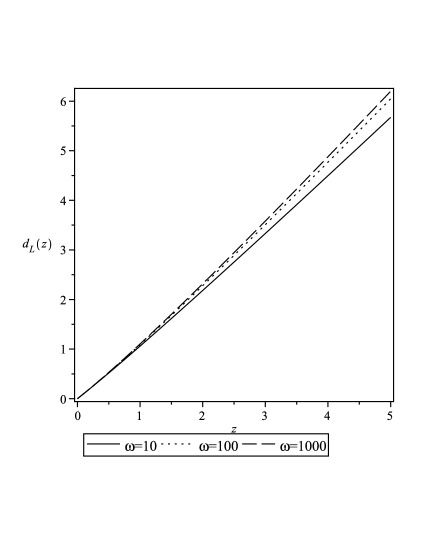
Figure 16: The behavior of the luminosity distance as a function of the redshift for values $\omega$.

V.4 Angular diameter

The angular diameter distance $d_{A}$ is simplified to

$$d_{A}=d_{L}(1+z)^{-2}.$$ (54)

The Figure-17 shows the variation of the angular diameter as a function of the exponent $0<n<1$.

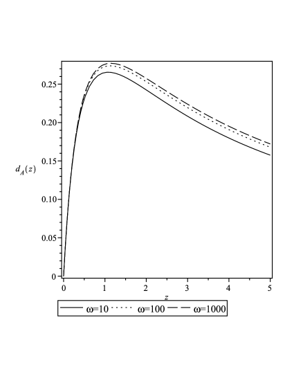
Figure 17: The behavior of the angular diameter as a function of the redshift for values $\omega$.

VI Conclusion

To recapitulate, we studied the Brans-Dicke Chameleon cosmology by obtaining exact solutions of the scale factor $a(t)$, scalar field $\phi(t)$, the potential $V(\phi)$ and the arbitrary function $f(\phi)$ for different epochs of the cosmic evolution. This analysis was performed by using ansatz for the above parameters. These were motivated since earlier studies of dark energy show that these cosmic parameters obey power-law form of the time parameter. Next we plotted these parameters for various values of the BD parameter in different cosmic epochs.

In figures 1 and 2, the scale factor is plotted is shown for different times. The positive and negative subscripts of $a(t)$ correspond to two values given in (29). The behavior of scalar field $\phi$ is plotted in figures 3 and 4. It is shown that the positive component of the field $\phi_{+}$ increases faster for small values of $\omega$ and vice versa for $\phi_{-}$. In figures 5 and 6, the expressions for $f_{+}$ and $f_{-}$ are plotted. It is observed that these functions behave more like exponential functions which shows that the coupling between the BD field and matter increases with time. In figures 7 and 8, we provide the behavior of the BD potential which is increasing (decreasing) for $V_{+}$ ($V_{-}$) against time for large (small) values of the BD parameter. Figure 9 gives the variation of the BD potential against the BD field while the figure 10 provides the variation of the scale factor in the limit when the BD parameters vanishes (becomes negligible).

In figures 11, 12 and 13, we have plotted statefinder parameters and the deceleration parameter of our model against the BD parameter. It is observed that deceleration parameter is positive, thereby producing a decelerated Universe. Though the model suggests the expansion of the Universe, yet the model does not explain cosmic acceleration. The stability analysis of the solutions is important. But it will be beyond the scope of our paper. Such analysis can be done using the similar methodology, as it has been done in stability1 , by defining dimensionless variables. The stability of BD with Chameleon field has been done already in stability2 for the same system of equations as we have.

References

- (1) C. H. Brans and R. H. Dicke, Phys. Rev. 124 (1961) 925.
- (2) K. Nordtvedt Jr, Ap. J. 161 (1970) 1059.
- (3) J. D. Benkestein et al, Phys. Rev. D 18 (1978) 4378.
- (4) J. M. Alimi et al, Phys. Rev. D 53 (1996) 3074.
- (5) C. Mathhiazhagan et al, Class. Quant. Grav. 1 (1984) L29.
- (6) P. M. Garnavich et al, Ap. J. 509 (1998) 74.
- (7) S. Perlmutter et al, Ap. J. 517 (1999) 565.
- (8) A. G. Riess et al, Aston. J. 116 (1999) 74.
- (9) Bodo Geyer , Sergei D. Odintsov , Sergio Zerbini , Phys.Lett. B460 (1999) 58-62; Shin’ichi Nojiri , Sergei D. Odintsov , Mod.Phys.Lett. A19 (2004) 1273-1280; M.C.B. Abdalla, M.E.X. Guimaraes and J.M. Hoff da Silva, The European Physical Journal C, Volume 55, Number 2, Pages 337-342(2008); Hyung Won Lee, Kyoung Yee Kim and Yun Soo Myung, The European Physical Journal C , Volume 71, Number 3, 1585(2011); Lixin Xu, Wenbo Li and Jianbo Lu ,The European Physical Journal C , Volume 60, Number 1, Pages 135-140 (2009).
- (10) B.K. Sahoo et al, Mod. Phys. Lett. A 18 (2003) 2725-2734; gr-qc/0211038.
- (11) J. Khoury and A. Weltman, Phys. Rev. Lett. 93 (2004) 171104; Phys. Rev. D 69 (2004) 044026.
- (12) T. P. Waterhouse, arXiv:astro-ph/0611816.
- (13) P. Brax, C. Van de Bruck et al, JCAP 0411 (2004) 004.
- (14) S. S. Gubser et al, Phys. Rev. D 70 (2004) 104001.
- (15) K. Karami et al, Gen. Relativ. Gravit. (2011) 43:27 39
- (16) H. Farajollahi et al, JCAP 05(2011)017.
- (17) Hossein Farajollahi et al, JCAP 1011:006,2010.
- (18) Sahni, V. et al, JETP. Lett. 77(2003)201.
- (19) Zhang, X, Int. J. Mod. Phys. D14(2005)1597.
- (20) Wei, H et al, Phys. Lett. B655(2007)1.
- (21) Zhang, X, Phys. Lett. B611(2005)1.
- (22) Huang, J.Z et al, Astrophys. Space Sci. 315(2008)175.
- (23) Zhao, W, Int. J . Mod. Phys. D17(2008)1245.
- (24) Hu, M. et al, Phys. Lett. B635(2006)186.
- (25) Zimdahl, W et al, Gen. Relativ. Gravit. 36(2004)1483.
- (26) Shao, Y et al, Mod. Phys. Lett. A23(2008)65.
- (27) Jamil, M et al, Int. J. Theor. Phys. 50 (2011) 1602.
- (28) M.R. Setare and M. Jamil, Gen. Relativ. Gravit. (2011) 43:293-303
- (29) Campos, M.de.: arXiv:0912.1143v2 [gr-qc].
- (30) Sharif, M et al, Astrophys. Space Sci (to appear).
-
(31)
H. Farajollahi et al, JCAP 1011:006,2010;
H. Farajollahi et al, arXiv:1009.5059v1 [gr-qc];
A.F. Bahrehbakhsh et al, Gen. Rel. Grav. 43 (2011) 847 -
(32)
M. Jamil et al, Phys. Lett. B 694 (2011)
284;
M.R. Setare and M. Jamil, Phys. Lett. B 690 (2010).