$K_{1}(1270)-K_{1}(1400)$ mixing and the fourth generation SM effects in $B\rightarrow K_{1}\ell^{+}\ell^{-}$ decays

Abstract

The implications of the fourth generation quarks in the $B\rightarrow K_{1}(1270,1400)\ell^{+}\ell^{-}$ with $\ell=\mu,\tau$ decays are studied, where the mass eigenstates $K_{1}(1270)$ and $K_{1}(1400)$ are the mixture of ${}^{1}{P}_{1}$ and ${}^{3}{P}_{1}$ states with the mixing angle $\theta_{K}$. In this context, we have studied various observables like branching ratio $(\mathcal{BR})$, forward backward asymmetry $(\mathcal{A}_{FB})$ and longitudinal and transverse helicity fractions $(f_{L,T})$ of $K_{1}$ meson in $B\to K_{1}\ell^{+}\ell^{-}$ decays. To study these observables, we have used the Light Cone QCD sum rules form factors and set the mixing angle $\theta_{K}=-34^{\circ}$. It is noticed that the $\mathcal{BR}$ is suppressed for $K_{1}(1400)$ as a final state meson compared to that of $K_{1}(1270)$. Same is the case when the final state leptons are tauons rather than muons. In both the situations all the above mentioned observables are quite sensitive to the fourth generation effects. Hence the measurements of these observables at LHC, for the above mentioned processes can serve as a good tool to investigate the indirect searches for the existence of fourth generation quarks.

I Introduction

The Standard Model (SM) with one Higgs boson is the simplest and has been tested with great precision. But with all of its successes, it has some theoretical shortcomings which impede its status as a fundamental theory. One such shortcoming is the so-called hierarchy problem, the various extensions and the SM differ in the solutions of this problem. These extensions are: the two Higgs doublet models (2HDM), Minimal Supersymmetric SM (MSSM), Universal Extra Dimension (UED) model and SM4. SM4, implying a fourth family of quarks and leptons seems to be the most economical in number of additional particles and simpler in the sense that it does not introduce any new operators. It thus provides a natural extension of the SM which has been searched for previously by the LEP and Tevatron and now will be investigated at the LHC 4sm . If a fourth family is discovered, it is likely to have consequences at least as profound as those that have emerged from the discovery of the third family. The fourth generation SM is not only provide a simple explanation of the experimental results which are difficult to reconcile with SM including CP violation anomaly 15 ; 16 but also give enough CP asymmetries to facilitate baryogenesis 18 . By the addition of fourth generation Cabibbo-Kobayashi-Maskawa (CKM) matrix become $4\times 4$ unitary matrix which requires six real parameters and three phases. These two extra phases imply the possibility of extra sources of CP violation. In addition, the fact that the heavier quarks ($t^{\prime},$ $b^{\prime}$) and leptons ($\nu^{\prime},$ $\ell^{\prime}$) of the fourth generation can play a crucial role in dynamical electroweak symmetry breaking (DEWSB) dewsb as an economical way to address the hierarchy puzzle which renders this extension of SM. Furthermore the LHC will provide a suitable amount of data which enlighten these puzzles more clearly as well as decide the faith of the extra generation to undimmed the smog from theoretical picture and help us to enhance our theoretical understanding.

In the past few years a number of analysis showed: (a) SM with fourth generation is consistent with the electroweak precision test (EWPT) 21 ; 22 ; 24 and it is pointed out in 22 ; 24 ; 27 that in the presence of fourth generation a heavy Higgs boson does not contradict with EWPT, (b) SU(5) gauge coupling unification could be achieved without supersymmetry 28 , (c) Electroweak baryogenesis can be accomodated 29 and (d) As mentioned earlier that the DEWSB might be actuated by the presence of extra generation dewsb . Moreover, the fourth generation SM, in principle, could resolve the certain anomalies present in flavor changing processes 39 . Also the mismatch in the $CP$ asymmetry in $B\to K\pi$ data hfag with the SM bashi2 as well as CP violation in $B\rightarrow\phi K_{s}$ decay may also provide some hint of new physics (NP) abds1 . Henceforth the measurement of different observables in the rare $B$ decays can also be very helpful to put or check the constraints on the $4$th generation parameters.

In general there are two ways to search the NP: one is the direct search where we can produce the new particles by raising the energy of colliders and the other one is indirect search, i.e. to increase the experimental precision on the data of different SM processes where the NP effects can manifest themselves. The processes that are suitable for indirect searches of NP are those which are forbidden or very rare in the SM and can be measured precisely. In this context the rare $B$ decays mediated through the flavor changing neutral current (FCNC) processes provide a potentially effective testing ground to look for the physics in and beyond the SM. In the SM, these FCNC transitions are not allowed at tree level but are allowed at loop level through Glashow-Iliopoulos-Maiani (GIM) mechanism GIM . In the context of SM, the rare $B$ decays are quite interesting because they provide a quantitative determination of the quark flavor rotation matrix, in particular the matrix elements $V_{tb}$, $V_{ts}$ and $V_{td}$ AAli .

The exploration of Physics beyond the SM through various inclusive $B$ meson decays like $B\to X_{s,d}\ell^{+}\ell^{-}$ and their corresponding exclusive processes, $B\to M\ell^{+}\ell^{-}$ with $M=K,K^{\ast},K_{1},\rho$ etc., have already been done bst ; 63 . These studies showed that the above mentioned inclusive and exclusive decays of $B$ meson are very sensitive to the flavor structure of the SM and provide a windowpane for any NP including the fourth generation SM. Therefore, the direct searches like the study of production, decay channels and the signals of the existence of fourth generation quarks and leptons in the present colliders are being performed. Since it is expected that $m_{t^{\prime}}>m_{t}$ thus the fourth generation quark can be manifest their indirect existence in the loop diagrams. Due to this reason FCNC transitions are at the forefront and one of the main research direction of all operating $B$ factories including CLEO, Belle, Tevatron and LHCb 4sm . However, the studies that involve the direct searches of the fourth generation quarks or their indirect searches via FCNC processes require the values of the quark masses and mixing elements which are not free parameters but rather they are constrained by experiments abds .

There are two different ways to incorporate the NP effects in the rare decays, one through the Wilson coefficients and the other through new operators which are absent in the SM. In the fourth generation SM the NP arises due to the modified Wilson coefficients $C_{7}^{eff}$ ,$C_{9}^{eff}$ and $C_{10}^{eff}$ as the fourth generation quark $(t^{\prime})$ contributes in $b\to s(d)$ transition at the loop level along with other quarks $u$, $c$ and $t$ of SM. It is necessary to mention here the FCNC decay modes like $B\rightarrow X_{s}\ell^{+}\ell^{-}$,$B\rightarrow K^{\ast}\ell^{+}\ell^{-}$ Kast and $B\rightarrow K\ell^{+}\ell^{-}$ are also very useful in the determination of precise values of $C_{7}^{eff}$ ,$C_{9}^{eff}$ and $C_{10}^{eff}$ Wilson coefficients inali as well as sign information on $C_{7}^{eff}$. Moreover, the measured branching ratio $b\rightarrow s\gamma$ by CLEO inali1 has been used to constraint the Wilson coefficient $C_{7}^{eff}$ bashi10 .

With our motivation stated above, the complementary information from the rare B decays is necessary for the indirect searches of NP including fourth generation. This complementary investigation improve the precession of SM parameters which are helpful in discovery of the NP. In this connection, like the rare semileptonic decays involving $B\rightarrow(X_{s},K^{\ast},K)\ell^{+}\ell^{-}$, the $B\rightarrow K_{1}(1270,1400)\ell^{+}\ell^{-}$ decays are also rich in phenomenology for the NP IPJ . In some sense they are more interesting and more sophisticated to NP since they are mixture of $K_{1A}$ and $K_{1B}$, where $K_{1A}$ and $K_{1B}$ are ${}^{3}P_{1}$ and ${}^{1}P_{1}$ states, respectively. The physical states $K_{1}(1270)$ and $K_{1}(1400)$ can be obtained by the mixing of $K_{1A}$ and $K_{1B}$ as

$$|K_{1}(1270)\rangle = |K_{1A}\rangle\sin{\theta_{K}}+|K_{1B}\rangle\cos{\theta_{K}},$$ (1a)

$$|K_{1}(1400)\rangle = |K_{1A}\rangle\cos{\theta_{K}}-|K_{1B}\rangle\sin{\theta_{K}},$$ (1b)

where the magnitude of mixing angel $\theta_{K}$ has been estimated to be $34^{\circ}\leq|\theta_{K}|\leq 58^{\circ}$ in Ref. Suzuki . Recently, from the study of $B\to K_{1}(1270)\gamma$ and $\tau\to K_{1}(1270)\nu_{\tau}$, the value of $\theta_{K}$ has been estimated to be $\theta_{K}=-(34\pm 13)^{\circ}$, where the minus sign of $\theta_{K}$ is related to the chosen phase of $|K_{1A}\rangle$ and $|K_{1B}\rangle$ HY . Getting an independent conformation of this value of mixing angle $\theta_{K}$ is by itself interesting. As we shall see that this particular choice suppresses the ${\cal BR}$ for $K_{1}(1400)$ in the final state compared to $K_{1}(1270)$, which can be tested.

Many studies have already shown IPJ that the observables like branching ratio $(\mathcal{BR})$, forward-backward asymmetry $(\mathcal{A}_{FB})$ and helicity fractions $f_{L,T}$ for semileptonic B decays are greatly influenced under different scenarios beyond the SM. Therefore, the precise measurement of these observables will play an important role in the indirect searches of NP. In this respect, it is natural to ask how these observables are influenced by the fourth generation parameters. The purpose of present study addresses this question i.e. investigate the possibility of searching NP due to the fourth generation SM in $B\rightarrow K_{1}(1270,1400)\ell^{+}\ell^{-}$ decays with $\ell=\mu,\tau$ using the above mentioned observables.

The plan of the manuscript is as follows. In sec. II, we fill our toolbox with the theoretical framework needed to study the said process in the fourth generation SM. In Sec. II.1, we present the mixing of $K_{1}(1270)$ and $K_{1}(1400)$ and the form factors used in this study. In Sec. III, we discuss the observables of $B\rightarrow K_{1}\ell^{+}\ell^{-}$ in detail. In Sec. IV, we give the numerical analysis of our observables and discuss the sensitivity of these observables with the fourth generation SM scenario. We conclude our findings in Sec. V.

II Theoretical Framework

At the quark level $B\rightarrow K_{1}(1270,1400)\ell^{+}\ell^{-}$ decays are induced by the transition $b\rightarrow s\ell^{+}\ell^{-}$, which in the SM, is described by the following effective Hamiltonian

$$\mathcal{H}_{eff} = -\frac{4G_{F}}{\sqrt{2}}V_{tb}V_{ts}^{\ast}\bigg{[}{\sum\limits_{i=1}^{10}}C_{i}({\mu})O_{i}({\mu})\bigg{]},$$ (2)

where $O_{i}({\mu})$ $(i=1,\ldots,10)$ are the four-quark operators and $C_{i}({\mu})$ are the corresponding Wilson coefficients at the energy scale ${\mu}$ Goto . Using renormalization group equations to resum the QCD corrections, Wilson coefficients are evaluated at the energy scale ${\mu=m}_{b}$. The theoretical uncertainties associated with the renormalization scale can be considerably reduced when the next-to-leading-logarithm corrections are included.

The explicit expressions of the operators responsible for exclusive $B\to K_{1}(1270,1400)\ell^{+}\ell^{-}$ decays are given by

$$O_{7} = \frac{e^{2}}{16\pi^{2}}m_{b}\left(\bar{s}\sigma_{\mu\nu}Rb\right)F^{\mu\nu},\$$ (3)

$$O_{9} = \frac{e^{2}}{16\pi^{2}}(\bar{s}\gamma_{\mu}Lb)(\bar{\ell}\gamma^{\mu}\ell),\$$ (4)

$$O_{10} = \frac{e^{2}}{16\pi^{2}}(\bar{s}\gamma_{\mu}Lb)(\bar{\ell}\gamma^{\mu}\gamma_{5}\ell),$$ (5)

with $R,L=\left(1\pm\gamma_{5}\right)/2$. In terms of the above Hamiltonian, the free quark decay amplitude for $b\rightarrow s\ell^{+}\ell^{-}$ can be written as:

$$\mathcal{M}_{SM}(b\rightarrow s\ell^{+}\ell^{-})=-\frac{G_{F}\alpha}{\sqrt{2}\pi}V_{tb}V_{ts}^{\ast}\bigg{\{}C_{9}^{effSM}(\bar{s}\gamma_{\mu}Lb)(\bar{\ell}\gamma^{\mu}\ell)$$

$$+C_{10}(\bar{s}\gamma_{\mu}Lb)(\bar{\ell}\gamma^{\mu}\gamma_{5}\ell)-2m_{b}C_{7}^{effSM}(\bar{s}i\sigma_{\mu\nu}\frac{q^{\nu}}{q^{2}}Rb)(\bar{\ell}\gamma^{\mu}\ell)\bigg{\}}$$ (6)

where $q$ is the momentum transfer. The operator $O_{10}$ can not be induced by the insertion of four-quark operators because of the absence of the neutral $Z$ boson in the effective theory. Hence, the Wilson coefficient $C_{10}$ is not renormalized under QCD corrections and therefore it is independent of the energy scale. In addition to this, the above quark level decay amplitude can take contributions from the matrix elements of four-quark operators, $\sum_{i=1}^{6}\langle\ell^{+}\ell^{-}s|O_{i}|b\rangle$, which are usually absorbed into the effective Wilson coefficient $C_{9}^{effSM}(\mu)$, which can be decomposed into the following three parts bst ; 63

$$C_{9}^{effSM}(\mu)=C_{9}(\mu)+Y_{SD}(z,s^{\prime})+Y_{LD}(z,s^{\prime}),$$

where the parameters $z$ and $s^{\prime}$ are defined as $z=m_{c}/m_{b},\,\,\,s^{\prime}=q^{2}/m_{b}^{2}$. $Y_{SD}(z,s^{\prime})$ describe the short-distance contributions from four-quark operators far away from the $c\bar{c}$ resonance regions, which can be calculated reliably in the perturbative theory. The long-distance contributions $Y_{LD}(z,s^{\prime})$ from four-quark operators near the $c\bar{c}$ resonance cannot be calculated from first principles of QCD and are usually parameterized in the form of a phenomenological Breit-Wigner formula, by making use of the vacuum saturation approximation and quark-hadron duality. The explicit expressions for $Y_{SD}(z,s^{\prime})$ and $Y_{LD}(z,s^{\prime})$ are

$$Y_{SD}(z,s^{\prime}) =h(z,s^{\prime})\{3C_{1}(\mu)+C_{2}(\mu)+3C_{3}(\mu)$$

$$+C_{4}(\mu)+3C_{5}(\mu)+C_{6}(\mu)\}$$

$$-\frac{1}{2}h(1,s^{\prime})\{4C_{3}(\mu)+4C_{4}(\mu)+3C_{5}(\mu)\}$$

$$-\frac{1}{2}h(0,s^{\prime})\{C_{3}(\mu)+3C_{4}(\mu)\}$$

$$+{\frac{2}{9}}\{3C_{3}(\mu)+C_{4}(\mu)+3C_{5}(\mu)+C_{6}(\mu)\},$$ (7)

with

$$h(z,s^{\prime}) =-{\frac{8}{9}}\mathrm{ln}z+{\frac{8}{27}}+{\frac{4}{9}}x-{\frac{2}{9}}(2+x)|1-x|^{1/2}$$

$$\times\left\{\begin{array}[]{l}\ln\left|\frac{\sqrt{1-x}+1}{\sqrt{1-x}-1}\right|-i\pi\quad\mathrm{for}{{\ }x\equiv 4z^{2}/s^{\prime}<1}\\ 2\arctan\frac{1}{\sqrt{x-1}}\qquad\mathrm{for}{{\ }x\equiv 4z^{2}/s^{\prime}>1}\end{array}\right.,$$ (10)

$$h(0,s^{\prime}) ={\frac{8}{27}}-{\frac{8}{9}}\mathrm{ln}{\frac{m_{b}}{\mu}}-{\frac{4}{9}}\mathrm{ln}s^{\prime}+{\frac{4}{9}}i\pi,$$ (11)

and

$$Y_{LD}\left(z,s^{\prime}\right)=\frac{3\pi}{\alpha^{2}}C^{(0)}\sum\limits_{V_{i}=\psi_{i}}\kappa_{i}\frac{m_{V_{i}}\Gamma\left(V_{i}\rightarrow l^{+}l^{-}\right)}{m_{V_{i}}^{2}-s^{\prime}m_{b}^{2}-im_{V_{i}}\Gamma_{V_{i}}}$$ (12)

where $C^{(0)}=3C_{1}+C_{2}+3C_{3}+C_{4}+3C_{5}+C_{6}$.

Irrespective to this, the non-factorizable effects bs1 from the charm loop can bring about further corrections to the radiative $b\rightarrow s\gamma$ transition, which can be absorbed into the effective Wilson coefficient $C_{7}^{effSM}$. Specifically, the Wilson coefficient $C^{effSM}_{7}$ takes the form chen

$$C_{7}^{eff}(\mu)=C_{7}(\mu)+C_{b\rightarrow s\gamma}(\mu),$$

with

$$C_{b\rightarrow s\gamma}(\mu) =i\alpha_{s}\bigg{[}{\frac{2}{9}}\eta^{14/23}(G_{1}(x_{t})-0.1687)-0.03C_{2}(\mu)\bigg{]},$$ (13)

$$G_{1}(x) ={\frac{x(x^{2}-5x-2)}{8(x-1)^{3}}}+{\frac{3x^{2}\mathrm{ln}^{2}x}{4(x-1)^{4}}},$$ (14)

where $\eta=\alpha_{s}(m_{W})/\alpha_{s}(\mu)$, $x=m_{t}^{2}/m_{W}^{2}$. $C_{b\rightarrow s\gamma}$ is the absorptive part for the $b\rightarrow sc\bar{c}\rightarrow s\gamma$ re-scattering and we have dropped out the small contributions proportional to CKM sector $V_{ub}V_{us}^{\ast}$. Furthermore, in the SM, the zero position of the forward-backward asymmetry depends only on the Wilson coefficients new2 which correspond to the short distance physics. In the present study, our focus is to determine the effects of the fourth family of quarks on different observables. As we will see the NP effects modify only the Wilson coefficients. Therefore, we will ignore the long distance charmonium $c\bar{c}$ contributions in our numerical calculation.

As noted in section I, the NP scenario provided by the fourth generation quarks is introduced on the same pattern as the three generations in the SM. Therefore, the operator basis are exactly the same as that of the SM, while the values of Wilson coefficients in Eq. (II) alter according to

$$C_{7}^{eff} = C_{7}^{effSM}+\frac{\lambda_{t^{\prime}}}{\lambda_{t}}C_{7}^{new},$$

$$C_{9}^{eff} = C_{9}^{effSM}+\frac{\lambda_{t^{\prime}}}{\lambda_{t}}C_{9}^{new},$$ (15)

$$C_{10}^{eff} = C_{10}+\frac{\lambda_{t^{\prime}}}{\lambda_{t}}C_{10}^{new},$$

where $\lambda_{t}=V^{\ast}_{tb}V_{ts}$ and $\lambda_{t^{\prime}}$ can be parameterized as:

$$\lambda_{t^{\prime}}=|V^{\ast}_{t^{\prime}b}V_{t^{\prime}s}|e^{i\phi},$$ (16)

where $\phi$ is the phase factor corresponding to the $b\to s$ transition in the fourth generation SM, which we set $90^{\circ}$ phi in the forthcoming numerical analysis of different physical observables. Here $V_{t^{\prime}b}$ and $V_{t^{\prime}s}$ are the elements of $4\times 4$ CKM extended matrix. The new contributions of the fourth generation up quark $t^{\prime}$ at loop level in $C_{7}^{eff}$, $C_{9}^{eff}$ and $C_{10}^{eff}$ in Eq. (15) can be obtained from the corresponding SM counterparts by trading, $m_{t}\to m_{t^{\prime}}$. The unitarity condition of $4\times 4$ CKM matrix now takes the form

$$V_{t^{\prime}b}V_{t^{\prime}s}^{\ast}=-(V_{ub}V_{us}^{\ast}+V_{cb}V_{cs}^{\ast}+V_{tb}V_{ts}^{\ast}).$$ (17)

If we define $\lambda_{f}=V_{fb}V_{fs}^{\ast}$ then the unitarity relation can be written in more elegant form

$$\lambda_{t^{\prime}}=-\left(\lambda_{u}+\lambda_{c}+\lambda_{t}\right)$$ (18)

Notice that this unitarity relation relates the unknown parameters in terms of the known parameters. Current theoretical bound on $\lambda_{t^{\prime}}$ value is $\lambda_{t^{\prime}}\leq 1.5\times 10^{-2}$ bound .

There are different limits on the lower bound of the fourth generation quark masses. The direct searches at the Tevatron constrained the $t^{\prime}$ mass, $m_{t^{\prime}}>256$GeV at $90\%$ C.L. CDF2 and by the decay of $b^{\prime}$ quark to t and $W^{-}$, they set a limit on $b^{\prime}$ mass, $m_{b^{\prime}}>338GeV$ at $95\%$ C.L. CDF1 . Present searches by CDF(D0) of fourth generation $t^{\prime}$ in their decays to $Wq$, have excluded $t^{\prime}$ quark with a mass below 335(296)GeV at $95\%$ CL CDF3 . In near future, we will see that these bounds could be considerably improved at LHC. Moreover, the fourth-generation quark masses are constrained by the perturbative unitarity of heavy-fermion scattering amplitudes chano to be $m_{t^{\prime}}\leq 500\sim 600$ GeV. However, in our numerical calculations, we set the bounds $300\leq m_{t^{\prime}}\leq 600$ GeV.

II.1 Form Factors and Mixing of $K_{1}(1270)-K_{1}(1400)$

The exclusive $B\rightarrow K_{1}(1270,1400)\ell^{+}\ell^{-}$ decays involve the hadronic matrix elements of quark operators given in Eq. (II) which can be parameterized in terms of the form factors as:

$$\left\langle K_{1}(k,\varepsilon)\left|V_{\mu}\right|B(p)\right\rangle =\varepsilon_{\mu}^{\ast}\left(M_{B}+M_{K_{1}}\right)V_{1}(q^{2})$$

$$-(p+k)_{\mu}\left(\varepsilon^{\ast}\cdot q\right)\frac{V_{2}(q^{2})}{M_{B}+M_{K_{1}}}$$

$$-q_{\mu}\left(\varepsilon\cdot q\right)\frac{2M_{K_{1}}}{q^{2}}\left[V_{3}(q^{2})-V_{0}(q^{2})\right]$$

$$\left\langle K_{1}(k,\varepsilon)\left|A_{\mu}\right|B(p)\right\rangle =\frac{2i\epsilon_{\mu\nu\alpha\beta}}{M_{B}+M_{K_{1}}}\varepsilon^{\ast\nu}p^{\alpha}k^{\beta}A(q^{2})$$ (20)

where $V_{\mu}=\bar{s}\gamma_{\mu}b$ and $A_{\mu}=\bar{s}\gamma_{\mu}\gamma_{5}b$ are the vectors and axial vector currents, involved in the transition matrix, respectively. Also $p(k)$ are the momenta of the $B(K_{1})$ mesons and $\varepsilon_{\mu}$ correspond to the polarization of the final state axial vector $K_{1}$ meson. In Eq.(LABEL:tf6) we have

$$V_{3}(q^{2})=\frac{M_{B}+M_{K_{1}}}{2M_{K_{1}}}V_{1}(q^{2})-\frac{M_{B}-M_{K_{1}}}{2M_{K_{1}}}V_{2}(q^{2})$$ (21)

with

$$V_{3}(0)=V_{0}(0)$$

In addition, there is also a contribution from the Penguin form factors which can be written as

$$\left\langle K_{1}(k,\varepsilon)\left|\bar{s}i\sigma_{\mu\nu}q^{\nu}b\right|B(p)\right\rangle$$

$$=\left[\left(M_{B}^{2}-M_{K_{1}}^{2}\right)\varepsilon_{\mu}-(\varepsilon\cdot q)(p+k)_{\mu}\right]F_{2}(q^{2})$$

$$+(\varepsilon^{\ast}\cdot q)\left[q_{\mu}-\frac{q^{2}}{M_{B}^{2}-M_{K_{1}}^{2}}(p+k)_{\mu}\right]F_{3}(q^{2})$$ (22)

$$\left\langle K_{1}(k,\varepsilon)\left|\bar{s}i\sigma_{\mu\nu}q^{\nu}\gamma_{5}b\right|B(p)\right\rangle=-i\epsilon_{\mu\nu\alpha\beta}\varepsilon^{\ast\nu}p^{\alpha}k^{\beta}F_{1}(q^{2})$$ (23)

with $F_{1}(0)=2F_{2}(0).$

As the physical states $K_{1}(1270)$ and $K_{1}(1400)$ are mixed states of the $K_{1A}$ and $K_{1B}$ with mixing angle $\theta_{K}$ as defined in Eqs. (1a-1b). The $B\to K_{1}$ form factors can be parameterized as

$$\left(\begin{array}[]{c}\langle K_{1}(1270)|\bar{s}\gamma_{\mu}(1-\gamma_{5})b|B\rangle\\ \langle K_{1}(1400)|\bar{s}\gamma_{\mu}(1-\gamma_{5})b|B\rangle\end{array}\right) = M\left(\begin{array}[]{c}\langle K_{1A}|\bar{s}\gamma_{\mu}(1-\gamma_{5})b|B\rangle\\ \langle K_{1B}|\bar{s}\gamma_{\mu}(1-\gamma_{5})b|B\rangle\end{array}\right),$$ (28)

$$\left(\begin{array}[]{c}\langle K_{1}(1270)|\bar{s}\sigma_{\mu\nu}q^{\mu}(1+\gamma_{5})b|B\rangle\\ \langle K_{1}(1400)|\bar{s}\sigma_{\mu\nu}q^{\mu}(1+\gamma_{5})b|B\rangle\end{array}\right) = M\left(\begin{array}[]{c}\langle K_{1A}|\bar{s}\sigma_{\mu\nu}q^{\mu}(1+\gamma_{5})b|B\rangle\\ \langle K_{1B}|\bar{s}\sigma_{\mu\nu}q^{\mu}(1+\gamma_{5})b|B\rangle\end{array}\right),$$ (33)

where the mixing matrix $M$ is

$$M=\left(\begin{array}[]{cc}\sin\theta_{K}&\cos\theta_{K}\\ \cos\theta_{K}&-\sin\theta_{K}\end{array}\right).$$ (34)

So the form factors $A^{K_{1}}$, $V_{0,1,2}^{K_{1}}$ and $F_{0,1,2}^{K_{1}}$ satisfy the following relation

$$\left(\begin{array}[]{c}\frac{A^{K_{1}(1270)}}{m_{B}+m_{K_{1}(1270)}}\\ \frac{A^{K_{1}(1400)}}{m_{B}+m_{K_{1}(1400)}}\end{array}\right) = M\left(\begin{array}[]{c}\frac{A^{K_{1A}}}{m_{B}+m_{K_{1A}}}\\ \frac{A^{K_{1B}}}{m_{B}+m_{K_{1B}}}\end{array}\right),$$ (39)

$$\left(\begin{array}[]{c}(m_{B}+m_{K_{1}(1270)})V_{1}^{K_{1}(1270)}\\ (m_{B}+m_{K_{1}(1400)})V_{1}^{K_{1}(1400)}\end{array}\right) = M\left(\begin{array}[]{c}(m_{B}+m_{K_{1A}})V_{1}^{K_{1A}}\\ (m_{B}+m_{K_{1B}})V_{1}^{K_{1B}}\end{array}\right),$$ (44)

$$\left(\begin{array}[]{c}\frac{V_{2}^{K_{1}(1270)}}{m_{B}+m_{K_{1}(1270)}}\\ \frac{V_{2}^{K_{1}(1400)}}{m_{B}+m_{K_{1}(1400)}}\end{array}\right) = M\left(\begin{array}[]{c}\frac{V_{2}^{K_{1A}}}{m_{B}+m_{K_{1A}}}\\ \frac{V_{2}^{K_{1B}}}{m_{B}+m_{K_{1B}}}\end{array}\right),$$ (49)

$$\left(\begin{array}[]{c}m_{K_{1}(1270)}V_{0}^{K_{1}(1270)}\\ m_{K_{1}(1400)}V_{0}^{K_{1}(1400)}\end{array}\right) = M\left(\begin{array}[]{c}m_{K_{1A}}V_{0}^{K_{1A}}\\ m_{K_{1B}}V_{0}^{K_{1B}}\end{array}\right),$$ (54)

$$\left(\begin{array}[]{c}F_{1}^{K_{1}(1270)}\\ F_{1}^{K_{1}(1400)}\end{array}\right) = M\left(\begin{array}[]{c}F_{1}^{K_{1A}}\\ F_{1}^{K_{1B}}\end{array}\right),$$ (59)

$$\left(\begin{array}[]{c}(m^{2}_{B}-m^{2}_{K_{1}(1270)})F_{2}^{K_{1}(1270)}\\ (m^{2}_{B}+m^{2}_{K_{1}(1400)})F_{2}^{K_{1}(1400)}\end{array}\right) = M\left(\begin{array}[]{c}(m^{2}_{B}+m^{2}_{K_{1A}})F_{2}^{K_{1A}}\\ (m^{2}_{B}+m^{2}_{K_{1B}})F_{2}^{K_{1B}}\end{array}\right),$$ (64)

$$\left(\begin{array}[]{c}F_{3}^{K_{1}(1270)}\\ F_{3}^{K_{1}(1400)}\end{array}\right) = M\left(\begin{array}[]{c}F_{3}^{K_{1A}}\\ F_{3}^{K_{1B}}\end{array}\right),$$ (69)

where we have supposed that $k^{\mu}_{K_{1}(1270),K_{1}(1400)}\simeq k^{\mu}_{K_{1A},K_{1B}}$.

For the numerical analysis we have used the light-cone QCD sum rules form factors fmf , summarized in Table 1, where the momentum dependence dipole parametrization is:

$$\mathcal{T}^{X}_{i}(q^{2})=\frac{\mathcal{T}^{X}_{i}(0)}{1-a_{i}^{X}\left(q^{2}/m^{2}_{B}\right)+b_{i}^{X}\left(q^{2}/m^{2}_{B}\right)^{2}}.$$ (70)

where $\mathcal{T}$ is $A$, $V$ or $F$ form factors and the subscript $i$ can take a value 0, 1, 2 or 3 the superscript $X$ belongs to $K_{1A}$ or $K_{1B}$ state.

$\mathcal{T}^{X}_{i}(q^{2})$	$\mathcal{T}(0)$	$a$	$b$	$\mathcal{T}^{X}_{i}(q^{2})$	$\mathcal{T}(0)$	$a$	$b$
$V_{1}^{K_{1A}}$	$0.34$	$0.635$	$0.211$	$V_{1}^{K_{1B}}$	$-0.29$	$0.729$	$0.074$
$V_{2}^{K_{1A}}$	$0.41$	$1.51$	$1.18$	$V_{1}^{K_{1B}}$	$-0.17$	$0.919$	$0.855$
$V_{0}^{K_{1A}}$	$0.22$	$2.40$	$1.78$	$V_{0}^{K_{1B}}$	$-0.45$	$1.34$	$0.690$
$A^{K_{1A}}$	$0.45$	$1.60$	$0.974$	$A^{K_{1B}}$	$-0.37$	$1.72$	$0.912$
$F_{1}^{K_{1A}}$	$0.31$	$2.01$	$1.50$	$F_{1}^{K_{1B}}$	$-0.25$	$1.59$	$0.790$
$F_{2}^{K_{1A}}$	$0.31$	$0.629$	$0.387$	$F_{2}^{K_{1B}}$	$-0.25$	$0.378$	$-0.755$
$F_{3}^{K_{1A}}$	$0.28$	$1.36$	$0.720$	$F_{3}^{K_{1B}}$	$-0.11$	$1.61$	$10.2$

Table 1: $B\to K_{1A,1B}$ form factors fmf , where $a$ and $b$ are the parameters of the form factors in dipole parametrization.

III Physical Observables

In this section, we calculate some interesting observables like the branching ratio $(\mathcal{BR})$, forward-backward asymmetry $(\mathcal{A}_{FB})$ as well as the helicity fractions of the final state $K_{1}$ meson and their sensitivity for the NP due to fourth generation SM,. From Eq. (II), one can get the decay amplitudes for $B\rightarrow K_{1}(1270)\ell^{+}\ell^{-}$ and $B\rightarrow K_{1}(1400)\ell^{+}\ell^{-}$ as

$$\mathcal{M}(B\rightarrow K_{1}\ell^{+}\ell^{-})=-\frac{G_{F}\alpha}{2\sqrt{2}\pi}V_{tb}V_{ts}^{\ast}\left[T_{V}^{\mu}\overline{\ell}\gamma_{\mu}\ell+T_{A}^{\mu}\overline{\ell}\gamma_{\mu}\gamma_{5}\ell\right]$$ (71)

where the functions $T_{A}^{\mu}$ and $T_{V}^{\mu}$ can be written in terms of matrix elements and then in auxiliary functions, as

$$T_{A}^{\mu} =C_{10}^{tot}\left\langle K_{1}(k,\epsilon)\left|\bar{s}\gamma^{\mu}\left(1-\gamma^{5}\right)b\right|B(p)\right\rangle$$ (72)

$$T_{V}^{\mu} =C_{9}^{tot}\left\langle K_{1}(k,\epsilon)\left|\bar{s}\gamma^{\mu}\left(1-\gamma^{5}\right)b\right|B(p)\right\rangle$$

$$-C_{7}^{tot}\frac{2im_{b}}{q^{2}}\langle K_{1}(k,\epsilon)\left|\bar{s}\sigma^{\mu\nu}\left(1+\gamma^{5}\right)q_{\nu}b\right|B(p)\rangle$$ (73)

$$T_{V}^{\mu} =f_{1}\epsilon^{\mu\nu\rho\sigma}\varepsilon_{\nu}^{\ast}p_{\rho}k_{\sigma}-if_{2}\varepsilon^{\ast\mu}-f_{3}(q\cdot\varepsilon)(p^{\mu}+k^{\mu})$$ (74)

$$T_{A}^{\mu} =\bigg{\{}f_{4}\epsilon^{\mu\nu\rho\sigma}\varepsilon_{\mu}^{\ast}p_{\rho}k_{\sigma}+if_{5}\varepsilon^{\ast\mu}$$

$$-if_{6}(q\cdot\varepsilon)(p^{\mu}+k^{\mu})+if_{0}(q\cdot\varepsilon)q^{\mu}\bigg{\}}$$ (75)

One can notice that by using the following Dirac equations of motion, the last term in the expression of $T_{V}^{\mu}$ will vanish,

$$q^{\mu}(\bar{\psi}_{1}\gamma_{\mu}\psi_{2})=(m_{2}-m_{1})\bar{\psi}_{1}\psi_{2}$$ (76)

$$q^{\mu}(\bar{\psi}_{1}\gamma_{\mu}\gamma_{5}\psi_{2})=-(m_{1}+m_{2})\bar{\psi}_{1}\gamma_{5}\psi_{2}$$ (77)

The auxiliary functions appearing in Eqs. (74) and (75) are defined as:

$$f_{1} = 4(m_{b}+m_{s})\frac{C_{7}^{eff}}{q^{2}}\bigg{\{}F_{1}^{K_{1A}}\sin\theta_{K}+F_{1}^{K_{1B}}\cos\theta_{K}\bigg{\}}+2C_{9}^{eff}\left\{\frac{A_{1}^{K_{1A}}\sin\theta_{K}}{m_{B}+m_{K_{1A}}}+\frac{A_{1}^{K_{1B}}\cos\theta_{K}}{m_{B}+m_{K_{1B}}}\right\}$$ (78)

$$f_{2} = 2(m_{b}+m_{s})\frac{C_{7}^{eff}}{q^{2}}\bigg{\{}(m_{B}^{2}-m^{2}_{K_{1A}})F_{2}^{K_{1A}}\sin{\theta_{K}}+(m_{B}^{2}-m^{2}_{K_{1B}})F_{2}^{K_{1B}}\cos{\theta_{K}}\bigg{\}}$$ (79)

$$+C_{9}^{eff}\bigg{\{}(m_{B}+m_{K_{1A}})V_{1}^{K_{1A}}\sin{\theta_{K}}+(m_{B}+m_{K_{1B}})V_{1}^{K_{1B}}\cos{\theta_{K}}\bigg{\}}$$

$$f_{3} = 2(m_{b}+m_{s})\frac{C_{7}^{eff}}{q^{2}}\left\{\left(F_{2}^{K_{1A}}+\frac{q^{2}F_{3}^{K_{1A}}}{m_{B}^{2}-m^{2}_{K_{1A}}}\right)\sin{\theta_{K}}+\left(F_{2}^{K_{1B}}+\frac{q^{2}F_{3}^{K_{1B}}}{m_{B}^{2}-m^{2}_{K_{1B}}}\right)\cos{\theta_{K}}\right\}$$ (80)

$$+C_{9}^{eff}\left(\frac{V_{2}^{K_{1A}}\sin{\theta_{K}}}{m_{B}+m_{K_{1A}}}+\frac{V_{2}^{K_{1B}}\cos{\theta_{K}}}{m_{B}+m_{K_{1B}}}\right)$$

$$f_{4} = 2C_{10}^{eff}\left(\frac{A^{K_{1A}}\sin{\theta_{K}}}{m_{B}+m_{K_{1A}}}+\frac{A^{K_{1B}}\cos{\theta_{K}}}{m_{B}+m_{K_{1B}}}\right)$$ (81)

$$f_{5} = C_{10}^{eff}\bigg{\{}(m_{B}+m_{K_{1A}})V_{1}^{K_{1A}}\sin{\theta_{K}}+(m_{B}+m_{K_{1B}})V_{1}^{K_{1B}}\cos{\theta_{K}}\bigg{\}}$$ (82)

$$f_{6} = C_{10}^{eff}\left(\frac{V_{2}^{K_{1A}}\sin{\theta_{K}}}{m_{B}+m_{K_{1A}}}+\frac{V_{2}^{K_{1B}}\cos{\theta_{K}}}{m_{B}+m_{K_{1B}}}\right)$$ (83)

$$f_{0} = 2\frac{C_{10}^{eff}}{q^{2}}\bigg{\{}m_{K_{1A}}\left(V_{3}^{K_{1A}}-V_{0}^{K_{1A}}\right)\sin{\theta_{K}}+m_{K_{1B}}\left(V_{3}^{K_{1B}}-V_{0}^{K_{1B}}\right)\cos{\theta_{K}}\bigg{\}}$$ (84)

III.1 Branching Ratio

The double differential decay rate for $B\rightarrow K_{1}\ell^{+}\ell^{-}$ can be written as HY ; Colangelo

$$\frac{d\Gamma}{dq^{2}d\cos\theta} = \frac{G_{F}^{2}\alpha^{2}}{2^{11}\pi^{5}m_{B}^{3}}\left|V_{tb}V_{ts}^{\ast}\right|^{2}u(q^{2})\times\left|\mathcal{M}\right|^{2}$$ (85)

with

$$\left|\mathcal{M}\right|^{2}=\mathcal{A}(q^{2})\cos^{2}\theta+\mathcal{B}(q^{2})\cos\theta+\mathcal{C}(q^{2})$$ (86)

and

$$u(q^{2})\equiv\sqrt{\lambda\left(1-\frac{4m_{\ell}^{2}}{q^{2}}\right)},\\$$ (87)

where

$$\lambda \equiv \lambda\left(m_{B}^{2},m_{K_{1}}^{2},q^{2}\right)$$

$$= m_{B}^{4}+m_{K_{1}}^{4}+q^{4}-2m_{K_{1}}^{2}m_{B}^{2}-2q^{2}m_{B}^{2}-2q^{2}m_{K_{1}}^{2}.$$

One can get the differential decay rate by performing the integration on $\cos\theta$ in Eq. (85), so

$$\frac{d\Gamma}{dq^{2}}=\frac{G_{F}^{2}\alpha^{2}}{2^{11}\pi^{5}m_{B}^{3}}\left|V_{tb}V_{ts}^{\ast}\right|^{2}\frac{1}{3}[2\mathcal{A}(q^{2})+6\mathcal{B}(q^{2})]$$ (89)

where

$$\mathcal{A}(q^{2}) =\frac{1}{2}\lambda(q^{2}-4m^{2})\left[|f_{1}|^{2}+|f_{4}|^{2}\right]-\frac{1}{m_{K_{1}}^{2}q^{2}}\left[|f_{2}|^{2}+|f_{5}|^{2}\right]-\frac{\lambda}{m_{K_{1}}^{2}q^{2}}\left[|f_{3}|^{2}+|f_{6}|^{2}\right]$$

$$+\frac{2\left(m_{B}^{2}-m_{K_{1}}^{2}-q^{2}\right)}{m_{K_{1}}^{2}q^{2}}\left\{\lambda\Re\left[f_{2}f_{3}^{\ast}\right]+\Re\left[f_{5}f_{6}^{\ast}\right]\right\}$$ (90)

$$\mathcal{B}(q^{2}) =4\Re\left[f_{1}f_{5}^{\ast}+f_{2}f_{4}^{\ast}\right]\sqrt{q^{2}(q^{2}-4m^{2})\lambda}$$ (91)

$$\mathcal{C}(q^{2}) =\frac{1}{2}(q^{2}-4m^{2})\lambda\left[|f_{1}|^{2}+|f_{4}|^{2}+8|f_{5}|^{2}\right]+4|f_{2}|^{2}(2m^{2}+q^{2})+\frac{\lambda}{m_{K_{1}}^{2}q^{2}}\left[|f_{2}+|f_{5}|^{2}+\lambda(|f_{3}|^{2}+|f_{6}|^{2})\right]$$

$$-2\Re(f_{2}f_{3}^{\ast})+|f_{0}|^{2}4m^{2}q^{2}+2\Re(f_{5}f_{6}^{\ast})\left[m_{B}^{2}-M_{K_{1}}^{2}-(4m^{2}-q^{2})\right]$$

$$-8m^{2}\Re(f_{5}f_{6}^{\ast})-\Re(f_{0}f_{6}^{*}(m_{B}^{2}+m_{K_{1}}^{2}))+\frac{1}{m_{K_{1}}^{2}}\left[|f_{6}|^{2}2m^{2}(2(m_{B}^{2}+m_{K_{1}}^{2}-q^{2}))\right]$$ (92)

The kinematical variables used in above equations are defined as $u=\left(p-p_{l^{-}}\right)^{2}-\left(p-p_{l^{+}}\right)^{2}$, $u=-u(q^{2})\cos\theta$. Here $\lambda$ is defined in Eq. (LABEL:lambda) and $\theta$ is the angle between the moving direction of $\ell^{+}$ and $B$ meson in the centre of mass frame of $\ell^{+}\ell^{-}$ pair.

It is also very useful to define the branching fractions $\mathcal{R}_{\ell}$ as:

$$\mathcal{R}_{\ell}=\frac{\mathcal{BR}(B\rightarrow K_{1}(1400)\ell^{+}\ell^{-})}{\mathcal{BR}(B\rightarrow K_{1}(1270)\ell^{+}\ell^{-})}$$ (93)

where $\ell=\mu,\ \tau$.

III.2 Forward-Backward Asymmetries

In this section we investigate the forward-backward asymmetry ($\mathcal{A}_{FB}$) of leptons. The measurement of the $\mathcal{A}_{FB}$ at LHC is significant due to the minimal form factors new2 hence this observable has great importance to check the more clear signals of any NP than the other observables such as branching ratio etc. In the context of fourth generation, the $\mathcal{A}_{FB}$ can also play a crucial role because it is driven by the loop top quark so it is sensitive to the fourth generation up type quark $t^{\prime}$ 63 .

The differential $\mathcal{A}_{FB}$ of final state lepton for the said decays can be written as

$${\frac{d\mathcal{A}_{FB}(q^{2})}{dq^{2}}}=\int_{0}^{1}\frac{d^{2}\Gamma}{dq^{2}d\cos\theta}d\cos\theta-\int_{-1}^{0}\frac{d^{2}\Gamma}{dq^{2}d\cos\theta}d\cos\theta$$ (94)

From experimental point of view the normalized forward-backward asymmetry is more useful, which is defined as

$$\mathcal{A}_{FB}=\frac{\int_{0}^{1}\frac{d^{2}\Gamma}{dq^{2}d\cos\theta}d\cos\theta-\int_{-1}^{0}\frac{d^{2}\Gamma}{dq^{2}d\cos\theta}d\cos\theta}{\int_{-1}^{1}\frac{d^{2}\Gamma}{dq^{2}d\cos\theta}d\cos\theta}$$

The differential $\mathcal{A}_{FB}$ for $B\rightarrow K_{1}\ell^{+}\ell^{-}$ decays can be obtained from Eq. (85), as

$$\frac{d\mathcal{A}_{FB}(q^{2})}{dq^{2}} = -\frac{G_{F}^{2}\alpha^{2}}{2^{11}\pi^{5}m_{B}^{3}}\left|V_{tb}V_{ts}^{\ast}\right|^{2}u\left(q^{2}\right)$$ (95)

$$\times\frac{3\mathcal{B}(q^{2})}{2\mathcal{A}(q^{2})+6\mathcal{C}_{1}(q^{2})}$$

where $\mathcal{A}(q^{2})$, $\mathcal{B}(q^{2})$ and $\mathcal{C}(q^{2})$ are defined in Eqs. $(\ref{aq},\ref{bq},\ref{cq})$.

III.3 Helicity Fractions of $K_{1}$ meson

We now discuss helicity fractions of $K_{1}(1270,1400)$ meson in $B\rightarrow K_{1}\ell^{+}\ell^{-}$ which are interesting observables and are insensitive to the uncertainties arising due to form factors and other input parameters. Thus the helicity fractions can be a good tool to test the NP beyond the SM. The final state meson helicity fractions were already discussed in the literature for $B\rightarrow K^{\ast}\left(K_{1}\right)\ell^{+}\ell^{-}$ decays Colangelo ; paracha .

The explicit expression of the longitudinal $(f_{L})$ and the transverse$(f_{T})$ helicity fractions for $B\rightarrow K_{1}\ell^{+}\ell^{-}$ decay can be obtained by trading $\left|\mathcal{M}\right|$ to $\left|\mathcal{M}_{L}\right|$ and $\left|\mathcal{M}_{\pm}\right|$, respectively, in Eq. (85). Here

$$\left|\mathcal{M}_{L}\right|^{2} = \mathcal{D}_{L}\cos^{2}\theta+\mathcal{E}_{L}$$ (96)

$$\left|\mathcal{M}_{\pm}\right|^{2} = \mathcal{D}_{\pm}\cos^{2}\theta+\mathcal{E}_{\pm}$$ (97)

By performing the integration on $\cos\theta$ in Eq. (85), we get

$$\frac{d\Gamma_{L}}{dq^{2}} =\frac{G_{F}^{2}\alpha^{2}}{2^{11}\pi^{5}}\frac{\left|V_{tb}V_{ts}^{\ast}\right|^{2}}{m_{B}^{3}}u(q^{2})\frac{2}{3}\left[\mathcal{D}_{L}(q^{2})+3\mathcal{E}_{L}(q^{2})\right]$$ (98)

$$\frac{d\Gamma_{\pm}}{dq^{2}} =\frac{G_{F}^{2}\alpha^{2}}{2^{11}\pi^{5}}\frac{\left|V_{tb}V_{ts}^{\ast}\right|^{2}}{m_{B}^{3}}u(q^{2})\frac{2}{3}[\mathcal{D}_{\pm}(q^{2})+3\mathcal{E}_{\pm}(q^{2})]$$ (99)

where $\mathcal{D}_{L}(q^{2})$, $\mathcal{D}_{\pm}(q^{2})$, $\mathcal{E}_{L}(q^{2})$ and $\mathcal{E}_{\pm}(q^{2})$ can be parameterized in terms of the auxiliary functions [c.f. Eqs. $(\ref{ax-a}-\ref{ax-d0})$] as

$$\mathcal{D}_{L}(q^{2}) =\frac{1}{2m^{2}_{K_{1}}}\left\{|f_{5}|^{2}\left[\left(m^{2}_{B}-m^{2}_{K_{1}}-q^{2}\right)^{2}-16m^{2}m^{2}_{K_{1}}\right]+|f_{2}|^{2}\left(2m^{2}_{K_{1}}q^{2}+\lambda\right)+\lambda^{2}|f_{3}|^{2}-8m^{2}\lambda|f_{5}|^{2}+4m^{2}q^{2}\lambda|f_{0}|^{2}\right.$$

$$\left.-2\Re(f_{5}f_{6}^{\ast})\left(m_{B}^{2}-m^{2}_{K_{1}}-q^{2}\right)\lambda-4\lambda\Re(f{2}f_{3}^{\ast})\left(m_{B}^{2}-m^{2}_{K_{1}}-q^{2}\right)+\lambda|f_{6}|^{2}\left[8\left(m_{B}^{2}+m^{2}_{K_{1}}-4q^{2}\right)m^{2}+\lambda\right]\right\}$$ (100)

$$\mathcal{D}_{+}(q^{2}) =\frac{1}{4}\left\{\left(q^{2}+4m^{2}\right)\left[\lambda|f_{4}|^{2}+4|f_{5}|^{2}+4\sqrt{\lambda}\left(\Im(f_{1}^{\ast}f_{2})+\Im(f_{4}^{\ast}f_{5})\right)\right]+(q^{2}-4m^{2})\left(\lambda|f_{1}|^{2}+4|f_{2}|^{2}\right)\right\}$$ (101)

$$\mathcal{D}_{-}(q^{2}) =\frac{1}{4}\left\{\left(q^{2}+4m^{2}\right)\left[\lambda|f_{1}|^{2}+|f_{2}|^{2}\right]+(q^{2}-4m^{2})\left[\lambda|f_{4}|^{2}+4\sqrt{\lambda}\left(\Im(f_{1}f_{2}^{\ast})+\Im(f_{4}f_{5}^{\ast})\right)\right]\right\}$$ (102)

$$\mathcal{E}_{L}(q^{2}) =\frac{1}{2m^{2}_{K_{1}}}\left\{\left(4m^{2}-q^{2}\right)\left[|f_{5}|^{2}\left(m^{4}_{B}-(m^{2}_{K_{1}}+q^{2})m_{B}^{2}\right)+|f_{2}|^{2}\left(m_{B}^{2}-m^{2}_{K_{1}}-q^{2}\right)^{2}+2\lambda^{2}\left(|f_{3}|^{2}+|f_{6}|^{2}\right)\right.\right.$$

$$\left.-4\lambda\left(m_{B}^{2}-m^{2}_{K_{1}}-q^{2}\right)\Re(f_{2}f_{3}^{\ast})\right]+q^{2}\lambda\Re(f_{5}f_{6}^{\ast})\left[\left(m_{B}^{2}-m^{2}_{K_{1}}\right)+4m^{2}-q^{2}\right]-4m^{2}\lambda\Im(f{5}f_{6}^{\ast})\left(m_{B}^{2}-m^{2}_{K_{1}}\right)$$

$$\left.+\left(m^{2}_{K_{1}}+q^{2}\right)|f_{5}|^{2}\left[q^{2}\left(4m^{2}-m^{2}_{K_{1}}-q^{2}\right)+4m^{2}\left(m^{2}_{K_{1}}+q^{2}\right)\right]\right\}$$ (103)

$$\mathcal{E}_{+}(q^{2}) =\frac{1}{4}\left(q^{2}-4m^{2}\right)\left\{\lambda\left(|f_{1}|^{2}+|f_{4}|^{2}\right)+\left(|f_{2}|^{2}+|f_{5}|^{2}\right)+4\sqrt{\lambda}\left(\Im(f_{1}^{\ast}f_{2})+\Im(f_{4}^{\ast}f_{5})\right)\right\}$$ (104)

$$\mathcal{E}_{-}(q^{2}) =\frac{1}{4}\left(q^{2}-4m^{2}\right)\left\{\lambda\left(|f_{1}|^{2}+|f_{4}|^{2}\right)+\left(|f_{2}|^{2}+|f_{5}|^{2}\right)+4\sqrt{\lambda}\left(\Im(f_{1}f_{2}^{\ast})+\Im(f_{4}f_{5}^{\ast})\right)\right\}$$ (105)

Finally the longitudinal and transverse helicity fractions become

$$f_{L}(q^{2}) = \frac{d\Gamma_{L}(q^{2})/dq^{2}}{d\Gamma(q^{2})/dq^{2}}$$ (106)

$$f_{\pm}(q^{2}) = \frac{d\Gamma_{\pm}(q^{2})/dq^{2}}{d\Gamma(q^{2})/dq^{2}}$$ (107)

$$f_{T}(q^{2}) = f_{+}(q^{2})+f_{-}(q^{2})$$ (108)

so that the sum of the longitudinal and transverse helicity amplitudes is equal to one i.e. $f_{L}(q^{2})+f_{T}(q^{2})=1$ for each value of $q^{2}$ Colangelo .

IV Numerical Results and Discussion

We present here our numerical results of the branching ratio ($\mathcal{BR}$), the forward backward asymmetry $(\mathcal{A}_{FB})$ and the helicity fractions ($f_{L,T})$ of $K_{1}(1270,1400)$ meson for the $B\rightarrow K_{1}(1270,1400)\ell^{+}\ell^{-}$ decays with $\ell=\mu,\tau$. Here we have taken the central values of all the input parameters. We first give the numerical values of input parameters which are used in our numerical calculations pdg :

$$m_{B}=5.28$$ GeV, GeV, GeV,

GeV, GeV, ,

, GeV^-2,

sec, GeV,

GeV, GeV,

GeV.

Besides these input parameters, the form factors (the scalar functions of the square of the momentum transfer), the non-perturbative quantities, which are also very important. To study the above mentioned physical observables we use the light cone QCD sum rules (LCQCD) form factors which are given in Table 1. In our numerical calculations, we set the mixing angle $\theta_{K}=-(34\pm 13)^{0}$ HY where we have taken the central value $\theta_{K}=-34^{0}$ and the values of the SM Wilson Coefficients at $\mu\sim m_{b}$ are given in Table 2.

$C_{1}$	$C_{2}$	$C_{3}$	$C_{4}$	$C_{5}$	$C_{6}$	$C_{7}$	$C_{9}$	$C_{10}$
1.107	-0.248	-0.011	-0.026	-0.007	-0.031	-0.313	4.344	-4.669

Table 2: The Wilson coefficients $C_{i}^{\mu}$ at the scale $\mu\sim m_{b}$ in the SM.

First, we discuss the $\mathcal{BR}$s of $B\rightarrow K_{1}(1270,1400)\mu^{+}\mu^{-}(\tau^{+}\tau^{-})$ decays which we have plotted as a function of $q^{2}$ (GeV${}^{2})$, shown in Figs. 1-4, both in the SM and in the fourth generation scenario. Figures 1 and 2 show the $\mathcal{BR}$ of $B\to K_{1}(1270)$ with $\mu^{+}\mu^{-}$ and $\tau^{+}\tau^{-}$ respectively and Figs. 3 and 4 show the same for $B\to K_{1}(1400)$. These figures depict that the values of $\mathcal{BR}$ strongly depend on the fourth generation effects which come through the new parameters (i.e the Wilson coefficients with $m_{t^{\prime}}$ instead of $m_{t}$ as well as from the $V_{t^{\prime}b}V_{t^{\prime}s}$ are encapsulated in Eq. (15)). One can see clearly from these graphs that the increment in the values of the fourth generation parameters, increase the value of the branching ratio accordingly, i.e. the $\mathcal{BR}$ is an increasing function of both $m_{t^{\prime}}$ and $V_{t^{\prime}b}V_{t^{\prime}s}$. Moreover, this constructive characteristic of the fourth generation effects to the $\mathcal{BR}$ manifest throughout the $q^{2}$ region irrespective to the mass of the final particles. In addition, one can also extract the constructive behavior of the fourth generation to the $\mathcal{BR}$ from Table 3. However, the quantitative analysis of the $\mathcal{BR}$ shows that the NP effects due to the fourth generation are comparatively more sensitive to the case of $B\rightarrow K_{1}(1270)\ell^{+}\ell^{-}$ than the case of $B\rightarrow K_{1}(1400)\ell^{+}\ell^{-}$.

Moreover, Table 3 shows that the maximum deviation (when we set $m_{t^{\prime}}=600$ GeV, $V_{t^{\prime}b}V_{t^{\prime}s}=1.5\times 10^{-3}$) from the SM value due to the fourth generation: for the case of $B\rightarrow K_{1}(1270)\mu^{+}\mu^{-}$ is approximately $6$ times, for the case of $B\rightarrow K_{1}(1270)\tau^{+}\tau^{-}$ is about $3.3$ times, for $B\rightarrow K_{1}(1400)\mu^{+}\mu^{-}$ is approximately $5.9$ time and for $B\rightarrow K_{1}(1400)\tau^{+}\tau^{-}$ is about $2.9$ times than that of SM values.

	$\mathcal{BR}(B\rightarrow K_{1}(1270)\mu^{+}\mu^{-})$, SM value: $1.97\times 10^{-6}$	$\mathcal{BR}(B\rightarrow K_{1}(1400)\mu^{+}\mu^{-})$, SM value: $5.76\times 10^{-8}$
$\ \ \ \ |V_{t^{\prime}b}V_{t^{\prime}s}|$ $3\times 10^{-3}$ $1.5\times 10^{-2}$	$m_{t^{\prime}}=300$      $m_{t^{\prime}}=500$     $m_{t^{\prime}}=600$ $2.01\times 10^{-6}$ $2.18\times 10^{-6}$ $2.38\times 10^{-6}$ $3.04\times 10^{-6}$ $7.43\times 10^{-6}$ $1.22\times 10^{-5}$	$m_{t^{\prime}}=300$      $m_{t^{\prime}}=500$      $m_{t^{\prime}}=600$ $5.88\times 10^{-8}$ $6.36\times 10^{-8}$ $6.90\times 10^{-8}$ $8.78\times 10^{-8}$ $2.09\times 10^{-7}$ $3.44\times 10^{-7}$
	$\mathcal{BR}(B\rightarrow K_{1}(1270)\tau^{+}\tau^{-})$, SM value: $6.06\times 10^{-8}$	$\mathcal{BR}(B\rightarrow K_{1}(1400)\tau^{+}\tau^{-})$, SM value: $9.39\times 10^{-10}$
$\ \ \ \ |V_{t^{\prime}b}V_{t^{\prime}s}|$ $3\times 10^{-3}$ $1.5\times 10^{-2}$	$\ \ \ \ m_{t^{\prime}}=300$      $m_{t^{\prime}}=500$      $m_{t^{\prime}}=600$ $6.14\times 10^{-8}$ $6.38\times 10^{-8}$ $6.62\times 10^{-8}$ $8.12\times 10^{-8}$ $1.39\times 10^{-7}$ $2.01\times 10^{-7}$	$m_{t^{\prime}}=300$      $m_{t^{\prime}}=500$      $m_{t^{\prime}}=600$ $9.51\times 10^{-10}$ $9.80\times 10^{-10}$ $1.01\times 10^{-9}$ $1.24\times 10^{-9}$ $1.98\times 10^{-9}$ $2.74\times 10^{-9}$

Table 3: The values of branching ratio of $B\to K_{1}(1270,1400)\ell^{+}\ell^{-}$ with $\ell=\mu,\ \tau$ for different values of $m_{t^{\prime}}$ and $\left|V^{\ast}_{t^{\prime}b}V_{t^{\prime}s}\right|$.

	$\mathcal{R}_{\mu}=\frac{\mathcal{BR}(B\rightarrow K_{1}(1400)\mu^{+}\mu^{-})}{\mathcal{BR}(B\rightarrow K_{1}(1270)\mu^{+}\mu^{-})}$, SM value: $2.92\times 10^{-2}$	$\mathcal{R}_{\tau}=\frac{\mathcal{BR}(B\rightarrow K_{1}(1400)\tau^{+}\tau^{-})}{\mathcal{BR}(B\rightarrow K_{1}(1270)\tau^{+}\tau^{-})}$, SM value: $1.54\times 10^{-2}$
$\ \ \ \ |V_{t^{\prime}b}V_{t^{\prime}s}|$ $3\times 10^{-3}$ $1.5\times 10^{-2}$	$m_{t^{\prime}}=300$      $m_{t^{\prime}}=500$     $m_{t^{\prime}}=600$ $2.92\times 10^{-2}$ $2.91\times 10^{-2}$ $2.90\times 10^{-2}$ $2.88\times 10^{-2}$ $2.81\times 10^{-2}$ $2.81\times 10^{-2}$	$m_{t^{\prime}}=300$      $m_{t^{\prime}}=500$      $m_{t^{\prime}}=600$ $1.54\times 10^{-2}$ $1.53\times 10^{-2}$ $1.52\times 10^{-2}$ $1.52\times 10^{-2}$ $1.42\times 10^{-2}$ $1.36\times 10^{-2}$

Table 4: The values of branching fractions $\mathcal{R}_{\ell}$, with $\ell=\mu,\tau$, for different values of $m_{t^{\prime}}$ and $\left|V^{\ast}_{t^{\prime}b}V_{t^{\prime}s}\right|$.

This is important to emphasis here that the increment in the branching ratio due to the fourth generation effect is optimally well separated than that of SM value. Furthermore the change in branching ratios due to the hadronic uncertainties as well as the uncertainty of the mixing angle $\theta_{K}$ are negligible in comparison of the NP effects. Therefore, any dramatically increment in the measurement of the branching ratio at present experiments will be a clear indication of NP. So the precise measurement of branching ratio is very handy tool to extract the information about the fourth generation parameters.

To observe the variation which comes through the fourth generation parameters in the branching fractions $\mathcal{R}_{\ell}=\mathcal{BR}(B\rightarrow K_{1}(1400)\ell^{+}\ell^{-})/\mathcal{BR}(B\rightarrow K_{1}(1270)\ell^{+}\ell^{-})$, with $\ell=\mu,\ \tau$, we draw the graph of $\mathcal{R}_{\mu}$ and $\mathcal{R}_{\tau}$ as a function of $q^{2}$ in Figs. 5 and 6. We have also summarized the numerical values of the branching fractions corresponding to the values of $m_{t^{\prime}}$ and $|V_{t^{\prime}b}V_{t^{\prime}s}|$ in Table 4. These numerical analysis shows that the branching fraction are insensitive to the NP. So this analysis support the argument that this observable is suitable to fix the value of $\theta_{K}$ HY .

($\mathbf{a}$)	($\mathbf{b}$)

Figure 1: The dependence of branching ratio of $B\to K_{1}(1270)\mu^{+}\mu^{-}$ on $q^{2}$ for different values of $m_{t^{\prime}}$ and $\left|V^{\ast}_{t^{\prime}b}V_{t^{\prime}s}\right|$. In all the graphs, the solid line corresponds to the SM, small dashed , medium dashed, long dashed correspond, $m_{t^{\prime}}=$ 300 GeV, 500 GeV and 600 GeV respectively. $\left|V^{\ast}_{t^{\prime}b}V_{t^{\prime}s}\right|$ has the value 0.003 and 0.015 in $(a)$ and $(b)$ respectively.

($\mathbf{a}$)	($\mathbf{b}$)

Figure 2: The dependence of branching ratio of $B\to K_{1}(1270)\tau^{+}\tau^{-}$ on $q^{2}$ for different values of $m_{t^{\prime}}$ and $\left|V^{\ast}_{t^{\prime}b}V_{t^{\prime}s}\right|$. The legends and the values of fourth generation parameters are same as in Fig. 1.

($\mathbf{a}$)	($\mathbf{b}$)

Figure 3: The dependence of branching ratio of $B\to K_{1}(1400)\mu^{+}\mu^{-}$ on $q^{2}$ for different values of $m_{t^{\prime}}$ and $\left|V^{\ast}_{t^{\prime}b}V_{t^{\prime}s}\right|$. The legends and the values of fourth generation parameters are same as in Fig. 1.

($\mathbf{a}$)	($\mathbf{b}$)

Figure 4: The dependence of branching ratio of $B\to K_{1}(1400)\tau^{+}\tau^{-}$ on $q^{2}$ for different values of $m_{t^{\prime}}$ and $\left|V^{\ast}_{t^{\prime}b}V_{t^{\prime}s}\right|$. The legends and the values of fourth generation parameters are same as in Fig. 1.

($\mathbf{a}$)	($\mathbf{b}$)

Figure 5: The dependence of branching fraction $\mathcal{R}_{\mu}=\mathcal{BR}(B\rightarrow K_{1}(1400)\mu^{+}\mu^{-})/\mathcal{BR}(B\rightarrow K_{1}(1270)\mu^{+}\mu^{-})$ on $q^{2}$ for different values of $m_{t^{\prime}}$ and $\left|V^{\ast}_{t^{\prime}b}V_{t^{\prime}s}\right|$. The legends and the values of fourth generation parameters are same as in Fig. 1.

($\mathbf{a}$)	($\mathbf{b}$)

Figure 6: The dependence of branching fraction $\mathcal{R}_{\tau}=\mathcal{BR}(B\rightarrow K_{1}(1400)\tau^{+}\tau^{-})/\mathcal{BR}(B\rightarrow K_{1}(1270)\tau^{+}\tau^{-})$ on $q^{2}$ for different values of $m_{t^{\prime}}$ and $\left|V^{\ast}_{t^{\prime}b}V_{t^{\prime}s}\right|$. The legends and the values of fourth generation parameters are same as in Fig. 1.

To illustrate the generic effects due to the fourth generation quarks on the forward-backward asymmetry $\mathcal{A}_{FB}$, we plot $\frac{d(\mathcal{A}_{FB})}{dq^{2}}$ as a function of $q^{2}$ in Figs. 7-10. As it is shown in Ref. HY that the zero position of the $\mathcal{A}_{FB}$ depends weakly on the value of $\theta_{K}$ but can be changed due to the variation of the NP scenarios. For the zero position of $\mathcal{A}_{FB}$ it is also argued that the uncertainty in the zero position of the $\mathcal{A}_{FB}$ is due to the hadronic uncertainties (form factors) is negligible new2 . Therefore, the zero position of the $\mathcal{A}_{FB}$ could also provide a stringent test for the NP effects.

In the present study Figs. 7 and 9 show the case of muons as final state leptons, the increment in the $|V_{t^{\prime}b}V_{t^{\prime}s}|$ and $m_{t^{\prime}}$ values shift the zero position of the $\mathcal{A}_{FB}$ towards the low $q^{2}$ region, this behavior is compatible with $B\to K^{\ast}\mu^{+}\mu^{-}$ decay vb . Moreover, the maximum values of $|V_{t^{\prime}b}V_{t^{\prime}s}|$ and $m_{t^{\prime}}$, shift the SM value ($2.8$ GeV²) of zero position of the $\mathcal{A}_{FB}$ for the case of $B\rightarrow K_{1}(1270)\mu^{+}\mu^{-}$ (see Fig. 7-b) to the value $2.1$ GeV². For the case of $B\rightarrow K_{1}(1400)\mu^{+}\mu^{-}$ (see Fig. 9-b) the zero position of the $\mathcal{A}_{FB}$ is shifted from its SM value (3.4 GeV²) to the value 2.4 GeV².

Besides the zero position of $\mathcal{A}_{FB}$, the magnitude of $\mathcal{A}_{FB}$ is also important tool (particularly, when the tauons are the final state leptons where the zero of the $\mathcal{A}_{FB}$ is absent) to investigate the NP. A closer look on the pattern of Figs. 7-10 tells us that the fourth generation parameters decrease the magnitude of $\mathcal{A}_{FB}$ from its SM value. The analysis of $\mathcal{A}_{FB}$ also demonstrate that in contrast to the $\mathcal{BR}$, the magnitude of the $\mathcal{A}_{FB}$ is decreasing function of the fourth generation parameters. It is clear from these graphs that decreasing behavior of the magnitude of $\mathcal{A}_{FB}$ is irrespective of the final state particles. It is suitable to comment here that just like the zero position of the $\mathcal{A}_{FB}$, the magnitude of $\mathcal{A}_{FB}$ depends on the values of the Wilson coefficient $C_{7},C_{9}$ and $C_{10}$. Thus the effects on the magnitude of $\mathcal{A}_{FB}$ are almost insensitive due to the uncertainties in the form factors. We noticed that the uncertainty due to the mixing angle $\theta_{K}$, magnitude of $\mathcal{A}_{FB}$ is mildly effected. On the other hand the change in the magnitude of $\mathcal{A}_{FB}$ due to the fourth generation are very prominent and easy to measure at the experiment. In the last, precise measurement of the zero position and the magnitude of $\mathcal{A}_{FB}$ are very good observables to yield any indirect imprints of NP including fourth generation.

($\mathbf{a}$)	($\mathbf{b}$)

Figure 7: The dependence of forward backward asymmetry of $B\to K_{1}(1270)\mu^{+}\mu^{-}$ on $q^{2}$ for different values of $m_{t^{\prime}}$ and $\left|V^{\ast}_{t^{\prime}b}V_{t^{\prime}s}\right|$. The legends and the values of fourth generation parameters are same as in Fig. 1.

($\mathbf{a}$)	($\mathbf{b}$)

Figure 8: The dependence of forward backward asymmetry of $B\to K_{1}(1270)\tau^{+}\tau^{-}$ on $q^{2}$ for different values of $m_{t^{\prime}}$ and $\left|V^{\ast}_{t^{\prime}b}V_{t^{\prime}s}\right|$. The legends and the values of fourth generation parameters are same as in Fig. 1.

($\mathbf{a}$)	($\mathbf{b}$)

Figure 9: The dependence of forward backward asymmetry of $B\to K_{1}(1400)\mu^{+}\mu^{-}$ on $q^{2}$ for different values of $m_{t^{\prime}}$ and $\left|V^{\ast}_{t^{\prime}b}V_{t^{\prime}s}\right|$. The legends and the values of fourth generation parameters are same as in Fig. 1.

($\mathbf{a}$)	($\mathbf{b}$)

Figure 10: The dependence of forward backward asymmetry of $B\to K_{1}(1400)\tau^{+}\tau^{-}$ on $q^{2}$ for different values of $m_{t^{\prime}}$ and $\left|V^{\ast}_{t^{\prime}b}V_{t^{\prime}s}\right|$. The legends and the values of fourth generation parameters are same as in Fig. 1.

We now discuss another interesting observable to get the complementary information about NP in $B\rightarrow K_{1}(1270,1400)\ell^{+}\ell^{-}$ transitions i.e. the helicity fractions of $K_{1}(1270,1400)$ produced in the final state. The measurement of longitudinally $K^{*}$ helicity fractions ($f_{L}$) in the decay modes $B\rightarrow K^{*}\ell^{+}\ell^{-}$ by BABAR collaboration with experimental error bab put enormous interest in this observable. Additionally, this is also shown that the helicity fractions of final state meson, just like $\mathcal{BR}$ and $\mathcal{A}_{FB}$, are also very good observables to dig out the NP Colangelo ; paracha . Current and future $B$ factories will accumulate more data on this observable which will be helpful not only to reduce the experimental errors but also to get any possible hint of NP from this observable. In this regard, it is natural to study the helicity fractions for the complementary FCNC processes like $B\rightarrow K_{1}(1270,1400)\ell^{+}\ell^{-}$ in and beyond the SM. For this purpose, we have plotted the longitudinal ($f_{L}$) and transverse ($f_{T}$) helicity fractions of $K_{1}(1270,1400)$ for SM and with different values of fourth generation parameters in Figs.(11-14). In these graphs the values of the longitudinal ($f_{L}$) and transverse ($f_{T}$) helicity fractions of $K_{1}(1270,1400)$ are plotted against $q^{2}$ and one can see clearly that at each value of $q^{2}$ the sum of $f_{L}$ and $f_{T}$ is equal to one.

Fig. 11 and 13 show the case of muons as final state leptons, the effects of the fourth generation on the longitudinal (transverse) helicity fractions of $K_{1}(1270)$ are marked up in the $0<q^{2}\leq 12$ GeV² region. On the other hand, for $K_{1}(1400)$ the effected region is $0<q^{2}\leq 6$ GeV². Here one can notice that the $q^{2}$ region of $K_{1}(1400)$ is smaller than that of $K_{1}(1270)$ but the fourth generation effects are more prominent. It is clear from these figures that although the influence of the fourth generation parameters on the maximum (minimum) values of the $K_{1}(1270,1400)$ helicity fractions are not very much effected (One can see from Figs. 11 and 13 that for the case of $B\to K_{1}(1270)\mu^{+}\mu^{-}$, the difference in the extremum values of helicity fractions , even at the maximum values of fourth generation parameters, is negligible to the SM value and for $B\to K_{1}(1400)\mu^{+}\mu^{-}$ the difference to the SM value is 0.09) but there is a reasonable shift in the position of these values which lies roughly at $q^{2}\simeq 1.8$ GeV² for SM. Figs. 13 and 14 also show that how the position of the maximum (minimum) values of $f_{L}$ ($f_{T}$) varies with the change in $m_{t^{\prime}}$ and $|V_{t^{\prime}b}V_{t^{\prime}s}|$ values. Furthermore, the position of these extremum values are shifted towards the low $q^{2}$ region and on setting the maximum values of the fourth generation parameters this shift in the position is approximately $0.9$ GeV². One more comment is necessary to mention here that like the zero position of the $\mathcal{A}_{FB}$, the position of the extremum values of the helicity fractions are not effected due to the uncertainty of the mixing angle $\theta_{K}$.

Now we turn our attention to the case, where tauns are the final state leptons and for this case the helicity fractions of $K_{1}(1270,1400)$ are plotted in Figs. 12 and 14. One can easily see that in contrast to the case of muons, there is no shift in the position of the extremum values of the helicity fractions, and are fixed at $q^{2}=12.5$ GeV². However, the change in the maximum (minimum) value of longitudinal (transverse) is more prominent as compare to the previous case where the muons are the final state leptons. These figures have also enlightened the variation in the extremum values of helicity fractions from the SM due to the change in the fourth generation parameters. The change in extremum values are very well marked up as compare to the uncertainties due to the mixing angle $\theta_{K}$ and the hadronic matrix element. For $B\to K_{1}(1270)\tau^{+}\tau^{-}$, the maximum setting of the fourth generation parameters the maximum (minimum) value of longitudinal (transverse) helicity fraction is changed from its SM value $0.51(0.49)$ to $0.72(0.28)$ and for $B\to K_{1}(1400)\tau^{+}\tau^{-}$ is changed from $0.76(0.24)$ to $0.92(0.06)$ which is suitable amount of change to measure.

The numerical analysis of helicity fractions shows that the measurement of the maximum (minimum) values of $f_{L}$ and $f_{T}$ and its position in the case of $B\to K_{1}(1270,1400)\tau^{+}\tau^{-}$ and $B\to K_{1}(1270,1400)\mu^{+}\mu^{-}$ respectively can be used as a good tool in studying the NP beyond the SM and the existence of the fourth generation quarks.

($\mathbf{a}$)	($\mathbf{b}$)
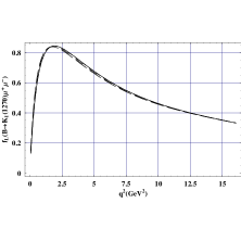
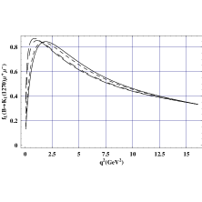
($\mathbf{c}$)	($\mathbf{d}$)

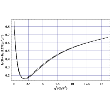
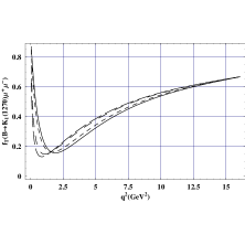
Figure 11: The dependence the probabilities of the longitudinal $(a,\ b)$ and transverse $(c,\ d)$ helicity fractions, $f_{L,T}$, of $K_{1}$ in $B\to K_{1}(1270)\mu^{+}\mu^{-}$ decays on $q^{2}$ for different values of $m_{t^{\prime}}$ and $\left|V^{\ast}_{t^{\prime}b}V_{t^{\prime}s}\right|$. In all the graphs, the solid line corresponds to the SM, small dashed , medium dashed, long dashed correspond, $m_{t^{\prime}}=$ 300 GeV, 500 GeV and 600 GeV respectively. $\left|V^{\ast}_{t^{\prime}b}V_{t^{\prime}s}\right|$ has the value 0.003 and 0.015 in $(a,c)$ and $(b,d)$ respectively.

($\mathbf{a}$)	($\mathbf{b}$)
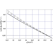
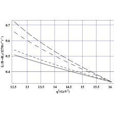
($\mathbf{c}$)	($\mathbf{d}$)

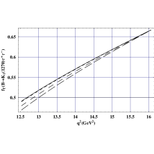
Figure 12: The dependence the probabilities of the longitudinal $(a,\ b)$ and transverse $(c,\ d)$ helicity fractions, $f_{L,T}$, of $K_{1}$ in $B\to K_{1}(1270)\tau^{+}\tau^{-}$ decays on $q^{2}$ for different values of $m_{t^{\prime}}$ and $\left|V^{\ast}_{t^{\prime}b}V_{t^{\prime}s}\right|$. The legends and the values of fourth generation parameters are same as in Fig. 11.

($\mathbf{a}$)	($\mathbf{b}$)
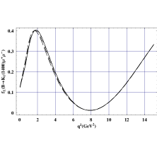
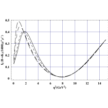
($\mathbf{c}$)	($\mathbf{d}$)

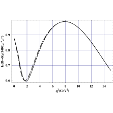
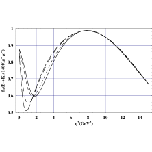
Figure 13: The dependence the probabilities of the longitudinal $(a,\ b)$ and transverse $(c,\ d)$ helicity fractions, $f_{L,T}$, of $K_{1}$ in $B\to K_{1}(1400)\mu^{+}\mu^{-}$ decays on $q^{2}$ for different values of $m_{t^{\prime}}$ and $\left|V^{\ast}_{t^{\prime}b}V_{t^{\prime}s}\right|$. The legends and the values of fourth generation parameters are same as in Fig. 11.

($\mathbf{a}$)	($\mathbf{b}$)
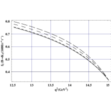
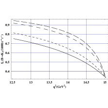
($\mathbf{c}$)	($\mathbf{d}$)

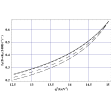
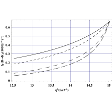
Figure 14: The dependence the probabilities of the longitudinal $(a,\ b)$ and transverse $(c,\ d)$ helicity fractions, $f_{L,T}$, of $K_{1}$ in $B\to K_{1}(1400)\tau^{+}\tau^{-}$ decays on $q^{2}$ for different values of $m_{t^{\prime}}$ and $\left|V^{\ast}_{t^{\prime}b}V_{t^{\prime}s}\right|$. The legends and the values of fourth generation parameters are same as in Fig. 11.

V Conclusion

In our study on the rare $B\rightarrow K_{1}(1270,1400)\ell^{+}\ell^{-}$ decays with $\ell=\mu$, $\tau$, we have calculated branching ratio ($\mathcal{BR}$), the forward backward asymmetry $\mathcal{A}_{FB}$ and helicity fractions $f_{L,T}$ of the final state mesons and analyzed the implications of the fourth generation effects on these observable for the said decays.

We have found a strong dependency of the $\mathcal{BR}$ on the fourth generation parameters $V_{t^{\prime}b}V_{t^{\prime}s}$ and $m_{t^{\prime}}$. The study has shown that the $\mathcal{BR}$ is an increasing function of these parameters. At maximum values of these parameters, i.e. $|V_{t^{\prime}b}V_{t^{\prime}s}|=0.015$ and $m_{t^{\prime}}=600$ GeV, the values of $\mathcal{BR}$ increases approximately 6 to 7 times larger than that of SM values when the final leptons are muons and for the case of of tauns these values are enhanced 3 to 4 times to the SM value. Hence the accurate measurement of the $\mathcal{BR}s$ value for these decays is very important tool to say something about the physics beyond the three generation of SM.

Besides the $\mathcal{BR}$, our analysis shown that $\mathcal{A}_{FB}$ is also a very good observable to check the existence of the fourth generation quarks, especially the zero position of the $\mathcal{A}_{FB}$. We have found that the value of the $\mathcal{A}_{FB}$ decreases with increases in the values of $V_{t^{\prime}b}V_{t^{\prime}s}$ and $m_{t^{\prime}}$. Moreover, the decrement in the values of the $\mathcal{A}_{FB}$ from the SM values are important imprints of NP and also the shift in the zero position of $\mathcal{A}_{FB}$ (which is towards low $q^{2}$ region) provides a prominent signature of the NP fourth generation quarks.

To comprehend the fourth generation effects on these decays, we have calculated the helicity fractions $f_{L,T}$ of final state mesons. We have first calculated these helicity fractions of final state mesons in the SM and then analyzed their extension to the fourth generation scenario. The study has shown that the deviation from the SM values of the helicity fractions are quite large when we set tauons as a final state of leptons. It is also shown that there is a noticeable change due to fourth generation in the position of the extremum values of the longitudinal and transverse helicity fractions of $K_{1}$ meson for the case of muons as a final state leptons. Therefore, the helicity fraction of $K_{1}$ meson can be a stringent test in finding the status of the fourth generation quarks.

Another attraction to consider the decay channel $B\to K_{1}\ell^{+}\ell^{-}$ is to get the complimentary information about the parameters of fourth generation SM to that of the information obtained from other experiments such as the inclusive $B\to X_{s}\ell^{+}\ell^{-}$ and the exclusive $B\to M(K,K^{\ast})\ell^{+}\ell^{-}$ decays. It is also worth mentioning here that the information obtained about the fourth generation parameters from the other experiments can be used to fix the mixing angle $\theta_{K}$ between the $K_{1}$ states in our process. Therefore, the fourth generation SM information obtained from the other experiments will not only compliment our results but can be useful to understand the mixing nature of $K_{1}(1270)$ and $K_{1}(1400)$ mesons.

To sum up, the more data to be available from Tevatron and LHCb will provide a powerful testing ground for the SM and the possible existence of the fourth generation quarks and also put some constraints on the fourth generation parameters such as $V_{t^{\prime}b}V_{t^{\prime}s}$ and $m_{t^{\prime}}$. Our analysis of the fourth generation on the observables for $B\to K_{1}\ell^{+}\ell^{-}$ decays are useful for probing or refuting the existence of fourth family of quarks.

References

- (1) P. Frampton et al., Phys. Rept. 330, (2000) 263 [hep-ph/9903387]; P.Q. Hung and M. Sher, Phys. Rev. D 77, 037302 (2008) [arXiv:0711.4353]; Y. Kikukawa et al., Prog. Theor. Phys. 122,401(2009) [arXiv:0901.1962]; D. Atwood et al., arXiv:1104.3874.
- (2) A. Soni, A. Alok, A. Giri, R. Mohanti, S. Nandi, arXiv:0807.1871 A. Soni, A. Kumar Alok, A. Giri, Rukmani Mohanta and S. Nandi, Phys. Lett. B 683:302-305,2010.
- (3) Possible role of the fourth family in B-decays has also been emphasized in, W. S. Hou, M. Nagashima, G. Raz and A. Soddu, JHEP 0609, 012, (2006); W. S. Hou, M. Nagashima and A. Soddu, Phys. Rev. Lett. 95, 141601, (2005); W. S. Hou, H. Nan Li, S. Mishima and Nagashima, Phys. Rev. Lett. 98, 131801, (2007) [hep-ph/061107]. Phys. Rev. D 76, 016004, (2007) [hep-ph/0610385].
- (4) W. S. Hou, arXiv:0803.1234; C. Jarlskog and R. Stora, Phys. Lett. B208, 288 (1988); F. del Aguila and J. A. Aguilar-Saavdra, Phys.Lett. B386, 241 (1996); F. del Aguila and J. A. Aguilar-Saavedra and G. C. Branco, Nucl. Phys. B510, 39, 1998; R. Fok and G. D. Kribs, arXiv:0803.4207.
- (5) B. Holdom, Phys. Rev. Lett. 57 (1986) 2496; C. T. Hill, M. A. Luty, and E. A. Paschos, Phys. Rev. D 43 (1991) 3011; S. F. king, Phys. Lett. B 234 (1990) 108; G. Burdman and L. Da Rold, JHEP 12 (2007) 086 [arXiv:0710.0623]; P. Q. Hung and C. Xiong, arXiv:0911.3890 and arXiv:0911.3892; B. Holdom, Phys. Lett. B 686 (2010).
- (6) M. Maltoni, V. A. Novikov, L. B. Okun, A. N. Rozanov, and M. I. Vysotsky, Extra quark-lepton generations and precision measurements, Phy. Lett. B 476 (2000) 107 [hep-ph/9911535]; J. Alwall et al., Eur. Phys. J. C 49 (2007) 791, hep-ph/0607115; M. S. Chanowitz,Phys. Rev. D 79 (2009) 113008 [arXiv:0904.3570]; V. A. Novikov, A. N. Rozanov, and M. I. Vysotsky, arXiv:0904.4570.
- (7) H.-J. He, N. Polonsky, and S.-f. Su, Extra families, Higgs spectrum and oblique corrections, Phys. Rev. D 64 (2001) 053004 [hep-ph/0102144].
- (8) G. D. Kribs, T. Plehn, M. Spannowsky, and T. M. P. Tait, Phys. Rev. D 76 (2007) 075016, 0706.3718.
- (9) M. Hashimoto, arXiv:1001.4335.
- (10) P. Q. Hung, Phys. Rev. Lett. 80 (1998) 3000-3003 [hep-ph/9712338].
- (11) W.-S. Hou, Chin. J. Phys. 47 (2009) 134 [arXiv:0803.1234]; Y. Kikukawa, M. Kohda, and J. Yasuda, Prog. Theor. Phys. 122 (2009) 401 [arXiv:0901.1962]; R. Fok and G. D. Kribs, Phys. Rev. D 78 (2008) 075023 [arXiv:0803.4207].
- (12) W.-S. Hou, M. Nagashima, and A. Spddu, Phys. Rev. D 72 (2005) 115007 [hep-ph/0508237]; W. S. Hou, M. Nagashima, and A. Spddu, Phys. Rev. D 76 (2007) 016004 [hep-ph/0610385]; A. Soni, A. K. Alok, A. Giri, R. Mohanta, and S. Nandi, arXiv:0807.1971.
- (13) Heavy Flavor Averaging Group, hep-ex/0603003.
- (14) M. Beneke, G. Buchalla, M. Neubert, and C. T. Sachrajda, Phys. Rev. Lett. 83, 1914 (1999); Nucl. Phys. B591, 313 (2000); B 606, 245 (2001); Y.Y. Keum, H-n. Li, and A. I. Sanda, Phys. Lett. B 504, 6 (2001); Phys. Rev. D 63, 054008 (2001); C.W. Bauer, I. Z. Rothstein, and I.W. Stewart, Phys. Rev. D 74, 034010 (2006). Rev. D 59, 057501 (1999).
- (15) Plenary talk by M. Yamauchi (Belle Collaboration) at ICHEP 2002; and B. Aubert et al. [BABAR Collaboration], hep-ex/0207070, contributed to ICHEP 2002 (see talk by J. Richman).
- (16) S. L. Glashow, J. Iliopoulos, and L. Maiani, Phys. Rev. D2, (1970) 1285.
- (17) A.Ali, C.Creub and T.Mannel, Report DESY 93-016 (ZU-TH 4/93, IKDA 93/5), published in Proceedings of the ECFA Workshop on a European B Meson Factory, Hamburg, Germany, 1993, Eds. R.Aleksan and A.Ali; C. S. Kim,T. Morozumi and A. I. Sanda, Phys. Rev. D 56(1997) 7240. A.Ali and G.Hiller, Euro. Phys. Jour. C 8 (1999) 619. A.Ali, H.Asatrian and C.Greub, Phys.Lett.B 429(1998)87.
- (18) C.S. Kim et al., Phys. Lett. B 218 (1989) 343; X. G. He et al., Phys. Rev. D 38 (1988) 814; B. Grinstein et al., Nucl. Phys. B 319 (1989) 271; N. G. Deshpande et al., Phys. Rev. D 39 (1989) 1461; P. J. O’Donnell and H. K. K. Tung, Phys. Rev. D 43 (1991) 2067; N. Paver and Riazuddin, Phys. Rev. D 45 (1992) 978; J. L. Hewett, Phys. Rev. D 53, 4964 (1996); T. M. Aliev, V. Bashiry, and M. Savci, Eur. Phys. J. C 35, 197 (2004); T. M. Aliev, V. Bashiry, and M. Savci, Phys. Rev. D 72, 034031 (2005); T. M. Aliev, V. Bashiry, and M. Savci, J. High Energy Phys. 05 (2004) 037; T. M. Aliev, V. Bashiry, and M. Savci, Phys. Rev. D 73, 034013 (2006); T. M. Aliev, V. Bashiry, and M. Savci, Eur. Phys. J. C 40, 505 (2005); F. Kruger and L. M. Sehgal Phys. Lett. B 380, 199 (1996); Y. G. Kim, P. Ko, and J. S. Lee, Nucl. Phys. B544, 64 (1999); Chuan-Hung Chen and C. Q. Geng, Phys. Lett. B 516, 327 (2001); V. Bashiry, Chin. Phys. Lett. 22, 2201 (2005); W.S. Hou, A. Soni and H. Steger, Phys. Lett. B 192, 441 (1987); W.S. Hou, R.S. Willey and A. Soni, Phys. Rev. Lett. 58, 1608 (1987) [Erratum-ibid. 60, 2337 (1987)]; T. Hattori, T. Hasuike and S. Wakaizumi, Phys. Rev. D 60, 113008 (1999); T.M. Aliev, D.A. Demir and N.K. Pak, Phys. Lett. B 389, 83 (1996); Y. Dincer, Phys. Lett. B 505, 89 (2001) and references therin; C.S. Huang, W.J. Huo and Y.L. Wu, Mod. Phys. Lett. A 14, 2453 (1999); C.S. Huang, W.J. Huo and Y.L. Wu, Phys. Rev. D 64, 016009 (2001).
- (19) A. Ali, T. Mannel and T. Morosumi, Phys. Lett. B 273, 505 (1991).
- (20) M. Ciuchini, G. Degrassi, P. Gambino and G.F. Giudice, Nucl. Phys. B 527, 21 (1998); F.M. Borzumati and C. Greub, Phys.
- (21) M. Beneke et al., Nucl. Phys. B 612 (2001) 25 [hep-ph/0106067]; A. Ali et al., Phys. Rev. D 66 (2002) 034002 [hep-ph/0112300]; T. Feldmann and J. Matias, JHEP 0301 (2003) 074 [hep-ph/0212158]; F. Kruger and J. Matias, Phys. Rev. D 71 (2005) 094009 [hep-ph/0502060]; C. Bobeth et al., JHEP 0807 (2008) 106 [arXiv:0805.2525]; U. Egede et al., JHEP 0811 (2008) 032 [arXiv:0807.2589]; C. H. Chen et al., Phys. Lett. B 670 (2009) 374 [arXiv:0808.0127]; A. K. Alok et al., JHEP 1002, 053 (2010) [arXiv:0912.1382]; A. K. Alok et al., arXiv:1008.2367; A. K. Alok et al., arXiv:1103.5344; W. Altmannshofer et al., JHEP 0901, 019 (2009).
- (22) A.J. Buras and M. M unz, Phys. Rev. D52 (1995) 186; M. Misiak, Nucl. Phys. B393 (1993) 23; Err. ibid. B439 (1995) 461.
- (23) M.S. Alam et.al. (CLEO Collaboration), Phys. Rev. Lett. 74 (1995) 2885; S. Ahmed et.al. (CLEO Collaboration), CLEO CONF 99 10 (hep ex/9908022); R. Barate et.al. (ALEPH Collaboration), Phys. Lett. B429 (1998) 169.
- (24) S. Sultansoy, hep-ph/0004271.
- (25) M. A. Paracha et al., Eur. Phys. J. C 52 (2007) 967 [arXiv:0707.0733]; I. Ahmed et al., Eur. Phys. J. C 54 (2008) 591 [arXiv:0802.0740]; I. Ahmed et al., Eur. Phys. J. C 71 (2011) 1521 [arXiv:1002.3860]; A. Saddique et al., Eur. Phys. J. C 56 (2008) 267 [arXiv:0803.0192]; M.Jamil Aslam and Riazuddin, Phys. Rev. D 66 (2002) 096005 [hep-ph/0209106]; V. Bashiry, K. Azizi, JHEP 1001:033, (2010) [arXiv:0903.1505].
- (26) M. Suzuki, Phys. Rev. D 47, 1252 (1993); L. Burakovsky and J. T. Goldman, Phys. Rev. D 57, 2879 (1998) [hep-ph/9703271]; H. Y. Cheng, Phys. Rev. D 67, 094007 (2003) [hep-ph/0301198]
- (27) H. Hatanaka and K. C. Yang, Phys. Rev. D 77, 094023 (2003) [arXiv:0804.3198]; H. Hatanaka and K. C. Yang, Phys. Rev. D 78 (2008) 074007 [arXiv:0808.3731[hep-ph]].
- (28) T. Goto et al., Phys. Rev. D 55 (1997) 4273; T.Goto et al., Phys. Rev. D 58 (1998) 094006; S.Bertolini et al., Nucl. Phys. B 353 (1991) 591.
- (29) D. Melikhov et al., Phys. Lett. B 430 (1998) 332 [hep-ph/9803343]; J. M. Soares, Nucl. Phys. B 367 (1991) 575; G. M. Asatrian and A. Ioannisian, Phys. Rev. D 54 (1996) 5642 [hep-ph/9603318]; J. M. Soares, Phys. Rev. D 53 (1996) 241 [hep-ph/9503285].
- (30) C. H. Chen and C. Q. Geng, Phys. Rev. D 64 (2001) 074001 [hep-ph/0106193].
- (31) A. Ali et al., Phys. Rev. D 61 (2000) 074024 [hep-ph/9910221]; G. Burdman, Phys. Rev. D 57 (1998) 4254 [hep-ph/9710550].
- (32) W. S. Hou et al., Phys. Rev. Lett. 98 131801 (2007) [hep-ph/0611107].
- (33) H. Chen and W. Huo, [arXiv:1101.4660]; S. Nandi and A. Soni, [arXiv:1011.6091]; S. K. Garg, S. K. Vempati, [arXiv:1103.1011]; A. K. Alok et al., [arXiv:1011.2634].
- (34) A. Lister, 35th International Conference of High Energy Physics, (2010) Paris, France, arXiv:1101.5992; [CDF collaboration], CDF 10110, http://www-cdf.fnal.gov/physics/new/top/confNotes/tprime-CDFnotePub.pdf.
- (35) T. Aaltonen et al., [CDF Collaboration], arXiv:0912.1057.
- (36) T. Aaltonen et al., [CDF Collaboration], arXiv:1103.2482.
- (37) M.S. Chanowitz et al., Phys. Lett. B 78 285 (1978).
- (38) K. C. Yang, Phys. Rev. D 78 (2008) 034018 [arXiv:0807.1171].
- (39) B. Aubert et al. [BABAR Collaboration], Phys. Rev. D 73, 092001 (2006) [arXiv:hep-ex/0604007].
- (40) P. Colangelo et al., Phys. Rev. D 74, (2006) 115006 [hep-ph/0610044]; A. Siddique et al., arXiv:0803.0192.
- (41) M. A. Paracha et al., arXiv:1101.2323 (2011).
- (42) K. Nakamura et al. (Particle Data Group), J. Phys. G 37, 075021 (2010).
- (43) V. Bashiry and F. Falahati, arXiv:0707.3242 (2007).