Bounds on strong field magneto-transport in three-dimensional composites

Abstract

This paper deals with bounds satisfied by the effective non-symmetric conductivity of three-dimensional composites in the presence of a strong magnetic field. On the one hand, it is shown that for general composites the antisymmetric part of the effective conductivity cannot be bounded solely in terms of the antisymmetric part of the local conductivity, contrary to the columnar case studied in [15]. So, a suitable rank-two laminate the conductivity of which has a bounded antisymmetric part together with a high-contrast symmetric part, may generate an arbitrarily large antisymmetric part of the effective conductivity. On the other hand, bounds are provided which show that the antisymmetric part of the effective conductivity must go to zero if the upper bound on the antisymmetric part of the local conductivity goes to zero, and the symmetric part of the local conductivity remains bounded below and above. Elementary bounds on the effective moduli are derived assuming the local conductivity and effective conductivity have transverse isotropy in the plane orthogonal to the magnetic field. New Hashin-Shtrikman type bounds for two-phase three-dimensional composites with a non-symmetric conductivity are provided under geometric isotropy of the microstructure. The derivation of the bounds is based on a particular variational principle symmetrizing the problem, and the use of $Y$-tensors involving the averages of the fields in each phase.

Keywords: bounds, homogenization, magneto-transport, strong field, multiphase composites.

AMS classification: 35B27, 74Q20

1 Introduction

It is known since the seminal discovery of Hall in the end of the 19th century [19], that a low magnetic field perturbs the matrix resistivity (or equivalently the conductivity) of a conductor by inducing a small non-symmetric part characterized by the so-called Hall coefficient. In the 80’s Bergman [5] first gave a general formula for the effective Hall coefficient involving currents that solve the symmetric conductivity equations in the absence of a magnetic field. However, there are few explicit formulas for the effective Hall coefficient except in very particular cases like two-phase two-dimensional composites [24, 6, 16], or columnar composites [7, 9, 31, 22, 23]. The situation is still less favorable in the strong field case [8, 10], namely when the symmetric part and the antisymmetric part of the conductivity are of the same order. In three dimensions, only when the antisymmetric part is constant do we have an exact formula for the antisymmetric part of the effective tensor [32]. So, rather than trying to get explicit relations for the effective tensors it seems more practical to derive bounds. The theory of the bounds in homogenization has gone through a considerable development since the original variational approach of Hashin and Shtrikman [20]. We refer to [26] for a comprehensive survey. In fact, very little is known about bounds for strong field magneto-transport. Recently, we derived in [15] optimal bounds for multiphase columnar composites. The aim of this paper is to extend, at least partially, the result of [15] to two-phase three-dimensional composites.

In the present context we consider a three-dimensional conductor having a periodic structure (this is actually not a restrictive assumption) in the presence of a fixed vertical strong magnetic field. Under the transverse isotropy assumption the local conductivity of the conductor takes the general form

$$\sigma(y)=\begin{pmatrix}a(y)&-c(y)&0\\ c(y)&a(y)&0\\ 0&0&b(y)\end{pmatrix},\quad\mbox{for }y\in\mathbb{R}^{3},$$ (1.1)

where the coefficient $c(y)$ is induced by the presence of the magnetic field parallel to the $y_{3}$-axis, which also influences $a(y)$ and $b(y)$ and causes them to be non-equal in the case of a conductor that is isotropic in the absence of the magnetic field. Similarly, assuming an transversely isotropic microstructure, or at least one that is invariant under $90^{\circ}$ or $120^{\circ}$ rotations about the $y_{3}$-axis, the constant effective conductivity of the composite is given by

$$\sigma_{*}=\begin{pmatrix}a_{*}&-c_{*}&0\\ c_{*}&a_{*}&0\\ 0&0&b_{*}\end{pmatrix}.$$ (1.2)

Our goal is to derive bounds for the effective coefficients $a_{*}$, $b_{*}$, $c_{*}$ of $\sigma_{*}$ in terms of the coefficients $a(y)$, $b(y)$, $c(y)$ of the local conductivity $\sigma(y)$.

In Section 2, we derive elementary bounds (see Theorem 2.1) on the effective coefficients $a_{*}$, $b_{*}$ and $c_{*}$. These are obtained by taking uniform trial fields in a variational principle for non-symmetric tensors deduced in [25, 18] from a symmetrization of the constitutive law $j=\sigma e$, and its adjoint, adapted from the variational approach performed in [17] for complex tensors.

In Section 3, we show (see Theorem 3.1) that contrary to the columnar case of [15], it is not possible to bound the antisymmetric part of the effective conductivity $\sigma_{*}$ only in terms of the coefficients $c(y)$. Indeed, when $\sigma(y)$ is independent of $y_{3}$ for a vertical columnar structure, the key ingredient for the derivation of the optimal bounds in [15] is based on the positivity of the $(2\times 2)$ determinant of the local electric field [1, 2], i.e.

$$\Delta_{1,2}(DU):=\partial_{1}u_{1}\,\partial_{2}u_{2}-\partial_{1}u_{2}\,\partial_{2}u_{1}>0\quad\mbox{a.e. in }\mathbb{R}^{3},$$ (1.3)

where the vector-valued potential $U=(u_{1},u_{2},u_{3})$ solves the conductivity problem

$$\left\{\begin{array}[]{ll}{\rm div}\left(\sigma DU\right)=0&\mbox{in }\mathbb{R}^{3}\\ U(y)-y&\mbox{is $Y$-periodic}.\end{array}\right.$$ (1.4)

Due to a suitably constructed rank-two laminate with high-contrast conductivity, we prove simultaneously that the inequality (1.3) does not hold, and that arbitrarily large effective coefficients $c_{*}$ can be obtained while the local coefficient $c(y)$ is bounded. This negative result agrees with the pathologies obtained in [13, 14] with different microstructures, related to bounds on the effective Hall coefficient in the low magnetic field regime. As a consequence, a bound for $c_{*}$ involves both the upper bound for $|c(y)|$ and the bounds from below and above for $a(y)$ in (1.1) (see Theorem 3.1 and Remark 3.2). This bound shows $c_{*}\to 0$ when the upper bound on $|c(y)|$ goes to zero, provided $a(y)$ remains bounded from below and above.

In Section 4, to improve the previous bounds we restrict ourselves to a two-phase local conductivity

$$\sigma(y)=\chi_{1}(y)\begin{pmatrix}a_{1}&-c_{1}&0\\ c_{1}&a_{1}&0\\ 0&0&b_{1}\end{pmatrix}+\chi_{2}(y)\begin{pmatrix}a_{2}&-c_{2}&0\\ c_{2}&a_{2}&0\\ 0&0&b_{2}\end{pmatrix},\quad\mbox{for }y\in\mathbb{R}^{3},$$ (1.5)

with prescribed volume fraction $f_{i}=\langle\chi_{i}\rangle$, for $i=1,2$, with $f_{1}+f_{2}=1$. We then derive (see Theorem 4.1) Hashin-Shtrikman type bounds for the effective conductivity $\sigma_{*}$, involving three intermediate coefficients $a_{Y}$, $b_{Y}$, $c_{Y}$ which are explicitly expressed in terms of the entries of $\sigma_{i}$, for $i=1,2,*$. In particular, it is shown that the point $(a_{Y},-c_{Y})$ belongs to a disk which is tangent to the axis $a=0$ at some point $(0,c)$, and which contains the disk passing through the points $(a_{1},c_{1})$, $(a_{2},c_{2})$, and tangent to the axis $a=0$ at the same point $(0,c)$ (see Figure 1 below). The derivation of these new bounds is based on a combination of three main ingredients:

• the geometric isotropy of the phases defined in [34] for random composites,

• the variational principle for non-symmetric tensors,

• the use of $Y$-tensors similar to [21] (see also [11]), giving relations between the averages of the fields in each phase.

Notations

• $(e_{1},e_{2},e_{3})$ denotes the canonic basis of $\mathbb{R}^{3}$.

• $I$ denotes the unit matrix of $\mathbb{R}^{3\times 3}$, and $J:=\left(\begin{smallmatrix}0&-1&0\\ 1&0&0\\ 0&0&0\end{smallmatrix}\right)$.

• For any matrix $M\in\mathbb{R}^{2\times 2}$, $M^{T}$ denotes the transpose of $M$, $M^{S}:=\frac{1}{2}\,\bigl{(}M+M^{T}\bigr{)}$ the symmetric part of $M$, and $M^{A}:=\frac{1}{2}\,\bigl{(}M-M^{T}\bigr{)}$ the antisymmetric part of $M$.

• $Y$ denotes the unit cube $[0,1]^{3}$, and $\langle\cdot\rangle$ the $Y$-average.

• For a function $f$ defined on the unit sphere $S^{2}$ of $\mathbb{R}^{3}$, $\langle f\rangle_{S^{2}}$ denotes the average of $f$ over $S^{2}$, i.e.

  $$\langle f\rangle_{S^{2}}:=\displaystyle-\mskip-19.2mu\int_{S^{2}}f(\xi)\,d\xi={1\over 4\pi}\int_{0}^{2\pi}d\varphi\int_{0}^{\pi}f(\sin\theta\cos\varphi,\sin\theta\sin\varphi,\cos\theta)\,\sin\theta\,d\theta.$$ (1.6)

• For $\alpha,\beta>0$, ${\cal M}_{\sharp}(\alpha,\beta;Y)$ denotes the set of the $Y$-periodic invertible matrix-valued functions $A:\mathbb{R}^{3}\to\mathbb{R}^{2\times 2}$ such that

  $$\forall\,\xi\in{\mathbb{R}^{3},}\quad A(y)\,\xi\cdot\xi\geq\alpha\,|\xi|^{2}\quad\text{and}\quad A^{-1}(y)\,\xi\cdot\xi\geq\beta^{-1}\,|\xi|^{2}\quad\text{a.e.~{}}y\in Y.$$ (1.7)

• $L^{2}_{\sharp}(Y)$ denotes the space of the $Y$-periodic functions, which are square integrable in $Y$.

• $H^{1}_{\sharp}(Y)$ denotes the space of the $Y$-periodic functions, with gradient in $L^{2}_{\sharp}(Y)^{3}$.

• For $u:\mathbb{R}^{3}\longrightarrow\mathbb{R}$, $\nabla u:=\bigl{(}\frac{\partial u}{\partial x_{i}}\bigr{)}_{1\leq i\leq 3}$.

• For $U:\mathbb{R}^{3}\longrightarrow\mathbb{R}^{3}$, $U=(u_{1},u_{2},u_{3})$, $DU:=\bigl{(}\frac{\partial u_{j}}{\partial x_{i}}\bigr{)}_{1\leq i,j\leq 3}$.

• For $\Sigma:\mathbb{R}^{3}\longrightarrow\mathbb{R}^{3\times 3}$, $\mathrm{div}\left(\Sigma\right):=\bigl{(}\frac{\partial\Sigma_{ij}}{\partial x_{i}}\bigr{)}_{1\leq j\leq 3}$.

2 Elementary bounds on magneto-transport

To derive bounds on composites we may assume that the associated microstructures are $Y$-periodic (see, e.g., [3] Theorem 1.3.23), where $Y$ is any cube of $\mathbb{R}^{3}$, say $Y=[0,1]^{3}$. In this section and the next we consider a three-dimensional $Y$-periodic conductor in the presence of a strong magnetic field parallel to the $y_{3}$-axis so that the resulting matrix-valued conductivity $\sigma(y)$ is given by

$$\sigma(y)=\begin{pmatrix}a(y)&-c(y)&0\\ c(y)&a(y)&0\\ 0&0&b(y)\end{pmatrix},\quad\mbox{for }y\in\mathbb{R}^{3},$$ (2.1)

where the coefficients $a(y),b(y),c(y)$ satisfy for prescribed positive numbers $\underline{a},\overline{a},\overline{c}>0$, with $\underline{a}\leq\overline{a}$, the following bounds

$$\underline{a}\leq a(y)\leq\overline{a}\quad\mbox{and}\quad|c(y)|\leq\overline{c},\qquad\mbox{a.e. }y\in\mathbb{R}^{3}.$$ (2.2)

By virtue of the periodic homogenization formula (see, e.g., [4]) the effective conductivity $\sigma_{*}$ associated with $\sigma(y)$ is given by

$$\sigma_{*}=\langle\sigma DU\rangle,\quad\mbox{where the potential $U$ solves }\quad\left\{\begin{array}[]{ll}{\rm div}\left(\sigma DU\right)=0&\mbox{in }\mathbb{R}^{3}\\ U(y)-y&\mbox{is $Y$-periodic}.\end{array}\right.$$ (2.3)

Recall that $\sigma_{*}$ is also the homogenized conductivity obtained from the oscillating sequence $\sigma({x\over\varepsilon})$ as $\varepsilon\to 0$ by a homogenization process (see, e.g., [4]).

Now consider a periodic electric field $e\in L^{2}_{\sharp}(Y)^{3}$ and a periodic current field $j\in L^{2}_{\sharp}(Y)^{3}$ that solves the conductivity equations

$$j=\sigma e,\quad{\rm div}~{}j=0,\quad{\rm curl}~{}e=0$$ (2.4)

and another periodic electric field $e^{\prime}\in L^{2}_{\sharp}(Y)^{3}$ and another periodic current field $j^{\prime}\in L^{2}_{\sharp}(Y)^{3}$ that solves the adjoint equations

$$j^{\prime}=\sigma^{T}e^{\prime},\quad{\rm div}~{}j^{\prime}=0,\quad{\rm curl}~{}e^{\prime}=0.$$ (2.5)

The average fields are related by the effective tensor $\sigma_{*}$:

$$\langle j\rangle=\sigma_{*}\langle e\rangle,\quad\langle j^{\prime}\rangle=\sigma_{*}^{T}\langle e^{\prime}\rangle.$$ (2.6)

Define the symmetric tensor

$$L(y):=\begin{pmatrix}(\sigma^{S})^{-1}&-\,(\sigma^{S})^{-1}\,\sigma^{A}\\ \vskip 6.0pt plus 2.0pt minus 2.0pt\cr\sigma^{A}\,(\sigma^{S})^{-1}&\sigma^{S}-\sigma^{A}\,(\sigma^{S})^{-1}\,\sigma^{A}\end{pmatrix}(y).$$ (2.7)

Then, an easy computation yields

$$F=\begin{pmatrix}e_{S}\\ j_{A}\end{pmatrix}=L\begin{pmatrix}j_{S}\\ e_{A}\end{pmatrix}=LE,\quad\mbox{where}\quad\left\{\begin{array}[]{ll}\displaystyle e_{S}:={1\over 2}\left(e+e^{\prime}\right),&\displaystyle e_{A}:={1\over 2}\left(e-e^{\prime}\right)\\ \vskip 6.0pt plus 2.0pt minus 2.0pt\cr\displaystyle j_{S}:={1\over 2}\left(j+j^{\prime}\right),&\displaystyle j_{S}:={1\over 2}\left(j+j^{\prime}\right).\end{array}\right.$$ (2.8)

Moreover, mimicking the approach of [17] for complex tensors, extended in [25, 18] (see also [26], p. 277) for real but non-symmetric tensors, the following variational principle holds

$$\begin{pmatrix}j_{0}\\ e_{0}\end{pmatrix}^{\!\!T}\!\!L_{*}\begin{pmatrix}j_{0}\\ e_{0}\end{pmatrix}=\min\left\{\left\langle\!\begin{pmatrix}j_{S}\\ e_{A}\end{pmatrix}^{\!\!T}\!\!L\begin{pmatrix}j_{S}\\ e_{A}\end{pmatrix}\!\right\rangle:{\left|\,\begin{array}[]{lll}e_{A}\in L^{2}_{\sharp}(Y)^{3},&\!\!{\rm curl}\left(e_{A}\right)=0,&\!\!\langle e_{A}\rangle=e_{0}\\ \vskip 6.0pt plus 2.0pt minus 2.0pt\cr j_{S}\in L^{2}_{\sharp}(Y)^{3},&\!\!{\rm div}\left(j_{S}\right)=0,&\!\!\langle j_{S}\rangle=j_{0}.\end{array}\right.}\!\!\right\},$$ (2.9)

with the symmetric effective tensor

$$L_{*}:=\begin{pmatrix}(\sigma_{*}^{S})^{-1}&-\,(\sigma_{*}^{S})^{-1}\,\sigma_{*}^{A}\\ \vskip 6.0pt plus 2.0pt minus 2.0pt\cr\sigma_{*}^{A}\,(\sigma_{*}^{S})^{-1}&\sigma_{*}^{S}-\sigma_{*}^{A}\,(\sigma_{*}^{S})^{-1}\,\sigma_{*}^{A}\end{pmatrix}.$$ (2.10)

By substituting constant trial fields $e_{A}=e_{0}$ and $j_{S}=j_{0}$ in the variational principle one immediately obtains the elementary bound

$$L_{*}\leq\langle L\rangle.$$ (2.11)

This elementary bound implies the following theorem:

Theorem 2.1.

Assuming $\sigma_{*}$ and $\sigma(y)$ have the forms (1.2) and (2.1) the constant $b_{*}$ must satisfy the arithmetic and harmonic mean bounds

$$1/\langle 1/b\rangle\leq b_{*}\leq\langle b\rangle,$$ (2.12)

and the pair $(a_{*},c_{*})$ must satisfy the circle bounds (which confine $(a_{*},c_{*})$ to lie within a circle in the $a_{*}$-$c_{*}$ plane) given by

$$(c_{*}-c_{L})^{2}\leq\left(a_{*}-a_{L}\right)\left(d_{L}-a_{*}\right),$$ (2.13)

where

$$a_{L}:=\left\langle{1\over a}\right\rangle^{-1},\quad c_{L}:=\left\langle{c\over a}\right\rangle a_{L},\quad d_{L}:=\left\langle a+{c^{2}\over a}\right\rangle-{c_{L}^{2}\over a_{L}}.$$ (2.14)

Remark 2.2.

Taking the minimum in (2.9) over all fields $e_{A}$ and $j_{S}$ with $\langle e_{A}\rangle=e_{0}$ and $\langle j_{S}\rangle=j_{0}$, and ignoring the differential constraints that ${\rm curl}\left(e_{A}\right)=0$ and ${\rm div}\left(j_{S}\right)=0$ gives the elementary bound $L_{*}^{-1}\leq\langle L^{-1}\rangle$. However this does not yield any new inequalities beyond (2.12) and (2.13) due to the structure of the matrices $L_{*}$ and $L(y)$.

Proof of Theorem 2.1. The proof follows the proof of the elementary bounds in Proposition 3.1 of [15]. Assuming $\sigma_{*}$ and $\sigma(y)$ have the forms (1.2) and (2.1) we obtain

$$L_{*}=\begin{pmatrix}\displaystyle{1\over a_{*}}&0&0&0&\displaystyle{c_{*}\over a_{*}}&0\\ 0&\displaystyle{1\over a_{*}}&0&\displaystyle-\,{c_{*}\over a_{*}}&0&0\\ 0&0&\displaystyle{1\over b_{*}}&0&0&0\\ 0&\displaystyle-\,{c_{*}\over a_{*}}&0&\displaystyle a_{*}+{c_{*}^{2}\over a_{*}}&0&0\\ \displaystyle{c_{*}\over a_{*}}&0&0&0&\displaystyle a_{*}+{c_{*}^{2}\over a_{*}}&0\\ 0&0&0&0&0&b_{*}\end{pmatrix}.$$ (2.15)

and

$$\langle L\rangle=\begin{pmatrix}\displaystyle{1\over a_{L}}&0&0&0&\displaystyle{c_{L}\over a_{L}}&0\\ 0&\displaystyle{1\over a_{L}}&0&\displaystyle-\,{c_{L}\over a_{L}}&0&0\\ 0&0&\left\langle\displaystyle{1\over b}\right\rangle&0&0&0\\ 0&\displaystyle-\,{c_{L}\over a_{L}}&0&\displaystyle d_{L}+{c_{L}^{2}\over a_{L}}&0&0\\ \displaystyle{c_{L}\over a_{L}}&0&0&0&\displaystyle d_{L}+{c_{L}^{2}\over a_{L}}&0\\ 0&0&0&0&0&\langle b\rangle\end{pmatrix}.$$ (2.16)

The matrix $\langle L\rangle-L_{*}$ will then be positive semi-definite if and only if (2.12) holds and

$$a_{*}\geq a_{L},$$ (2.17)

$$\left({c_{L}\over a_{L}}-{c_{*}\over a_{*}}\right)^{2}\displaystyle\leq\left({1\over a_{L}}-{1\over a_{*}}\right)\left(d_{L}+{c^{2}_{L}\over a_{L}}-a_{*}-{c_{*}^{2}\over a_{*}}\right)$$ (2.18)

By multiplying the last inequality by $a_{*}a_{L}$ and expanding (and using the fact that $a_{*}a_{L}>0$) we get (2.13). Also the inequality (2.17) is superfluous as it is implied by (2.13) and the inequality $d_{L}\geq a_{L}$.

3 Bounds on magneto-transport: 2d versus 3d

From (2.2) and the non-negativity of the 4th (or 5th) diagonal element of $\langle L\rangle-L_{*}$ we deduce the additional (superfluous) bound

$$2\,|c_{*}|\leq a_{*}+{c_{*}^{2}\over a_{*}}\leq\left\langle a+{c^{2}\over a}\right\rangle\leq\overline{a}+{\overline{c}^{2}\over\underline{a}},$$ (3.1)

where to obtain the first inequality we have used the fact that $x+1/x\geq 2$ for all $x>0$. Thus, we have obtained an upper bound on $|c_{*}|$, but one that involves not only $\overline{c}$ but also $\overline{a}$ and $\underline{a}$. This is in contrast to the case for a columnar conductivity $\sigma(y)$ which is independent of the $y_{3}$-variable, where using the positivity of the determinant of the electric field $DU(y)=DU(y_{1},y_{2})$ established by Alessandrini and Nesi [1, 2], we proved in [15] that $c_{*}$ satisfies the same bound $\overline{c}$ as the local coefficient $c(y)$ (i.e., $|c_{*}|\leq\overline{c}$).

Let us now relax the assumption that the effective tensor takes the form (1.2). The composite is said to be partially isotropic if the antisymmetric part of $\sigma_{*}$ satisfies

$$(\sigma_{*})^{A}=c_{*}\,J,\quad\mbox{where}\quad J:=\begin{pmatrix}0&-1&0\\ 1&0&0\\ 0&0&0\end{pmatrix}.$$ (3.2)

Given a partially isotropic composite we can always subdivide it into square columns with edges parallel to the $y_{3}$-axis and with side length much larger than the existing microstructure, and then rotate each square column about its center axis by either $0^{\circ}$, $90^{\circ}$, $180^{\circ}$ or $270^{\circ}$ with equal probability in an uncorrellated way. The resulting polycrystal is invariant under rotations of $90^{\circ}$ about the $y_{3}$-axis and thus will have an effective tensor of the form (1.2) and by a lemma of Stroud and Bergman [32] will have the same constant $c_{*}$ as the original partially isotropic composite.

The question naturally arises as to whether for partially isotropic composites $|c_{*}|$ can be bounded solely in terms of $\overline{c}$, like in the case of a columnar conductivity $\sigma(y)$? The answer is no, it cannot. Indeed, we have the following result:

Theorem 3.1.

Consider a periodic conductivity $\sigma(y)$ given by (2.1) which satisfies the bounds (2.2). Assume that the composite is partially isotropic in the sense of (3.2). Then, the effective coefficient $c_{*}$ satisfies

$$|c_{*}|\leq\frac{\overline{c}}{\underline{a}}\left(\sigma_{*}e_{1}\cdot e_{1}\right)^{1/2}\left(\sigma_{*}e_{2}\cdot e_{2}\right)^{1/2}.$$ (3.3)

On the other hand, given any arbitrarily large constant $\kappa>0$ there exist transversely isotropic conductivities $\sigma_{\theta,\kappa}(y)$ depending on a parameter $\theta>0$, with $c(y)\in\{0,1\}$ a.e. $y\in\mathbb{R}^{3}$, such that as $\theta\to 0$ the effective conductivity $\sigma_{\theta,\kappa}^{*}$ is partially isotropic and satisfies

$$\lim_{\theta\to 0}\,(\sigma_{\theta,\kappa}^{*})^{A}=-\kappa\,J\quad\mbox{or}\quad\lim_{\theta\to 0}\,(\sigma_{\theta,\kappa}^{*})^{A}=\kappa\,J.$$ (3.4)

Remark 3.2.

In the case when $\sigma_{*}$ is transversely isotropic, taking the form (1.2), the bound (3.3) reduces to

$$|c_{*}|\leq\frac{a_{*}}{\underline{a}}\,\overline{c},$$ (3.5)

and using (3.1) we obtain that

$$|c_{*}|\leq\frac{\overline{c}}{\underline{a}}\left(\left\langle a+{c^{2}\over a}\right\rangle-{c_{*}^{2}\over a_{*}}\right)\leq\frac{\overline{c}}{\underline{a}}\left(\displaystyle\overline{a}+{\overline{c}^{2}\over\underline{a}}\right).$$ (3.6)

In contrast to the bounds (3.1) and (2.13) this new bound shows that $c_{*}$ necessarily goes to zero as $\overline{c}$ goes to zero if $\overline{a}$ and $\underline{a}$ are held fixed. Also if we add the antisymmetric matrix $c_{0}J$ to $\sigma(y)$ then the effective tensor will change to $\sigma_{*}+c_{0}J$, implying from (3.5) that the inequality

$$|c_{*}+c_{0}|\leq\frac{a_{*}}{\underline{a}}\,\max\big{(}|c_{+}+c_{0}|,|c_{-}+c_{0}|\big{)}$$ (3.7)

holds for all constants $c_{0}$, where

$$c_{+}:=\sup_{y\in Y}c(y),\quad c_{-}:=\inf_{y\in Y}c(y).$$ (3.8)

Taking the optimum value $c_{0}=-(c_{+}+c_{-})/2$ gives the bounds

$$\left|2\,c_{*}-c_{+}-c_{-}\right|\leq\frac{a_{*}}{\underline{a}}\,(c_{+}-c_{-}).$$ (3.9)

Remark 3.3.

Theorem 3.1 proves that contrary to the columnar case of [15] we cannot expect to bound the effective coefficient $c_{*}$ only in terms of the bound $\overline{c}$ of the local coefficient $c(y)$. Actually, (3.4) shows that arbitrarily large (positive or negative) effective coefficients $c_{*}$ can be derived although the local coefficient $c(y)$ only takes values in $\{0,1\}$. Here, the contrast of the symmetric part of the conductivity plays a crucial role as suggested in the bound (3.3). This is strongly linked to the fact that the $(2\times 2)$ determinant

$$\Delta_{1,2}(DU):=\partial_{1}u_{1}\,\partial_{2}u_{2}-\partial_{1}u_{2}\,\partial_{2}u_{1},\quad\mbox{for }U=(u_{1},u_{2},u_{3}),$$ (3.10)

does not always have a constant sign throughout the material (see the proof of Theorem 3.1 below) contrary to the columnar case.

Proof of Theorem 3.1.

Bound for $c_{*}$: The div-curl lemma of Murat-Tartar (see [33, 29, 30]) and the formula (2.3) for $\sigma_{*}$ yield

$$\big{\langle}(DU)^{T}\sigma DU\big{\rangle}=\big{\langle}(DU)^{T}\big{\rangle}\,\big{\langle}\sigma DU\big{\rangle}=\big{\langle}DU\rangle^{T}\sigma_{*}\big{\langle}DU\big{\rangle}=\sigma_{*}.$$ (3.11)

Hence passing to the antisymmetric part it follows that

$$(\sigma_{*})^{A}=\big{\langle}(DU)^{T}\sigma^{A}DU\big{\rangle}=\big{\langle}c\,(DU)^{T}JDU\big{\rangle}=\left\langle c\left(\begin{smallmatrix}0&-\Delta_{1,2}(DU)&-\Delta_{1,3}(DU)\\ \Delta_{1,2}(DU)&0&-\Delta_{2,3}(DU)\\ \Delta_{1,3}(DU)&\Delta_{2,3}(DU)&0\end{smallmatrix}\right)\right\rangle,$$ (3.12)

where $\Delta_{i,j}(DU):=\partial_{1}u_{i}\,\partial_{2}u_{j}-\partial_{1}u_{j}\,\partial_{2}u_{i}$. Therefore, since $\sigma_{*}$ is partially isotropic, we obtain the following formula for the effective coefficient $c_{*}$,

$$c_{*}=\big{\langle}c\,\Delta_{1,2}(DU)\big{\rangle}.$$ (3.13)

Using the Cauchy-Schwartz inequality we have

$$\begin{array}[]{ll}|c_{*}|&\leq\overline{c}\left\langle\begin{pmatrix}|\partial_{1}u_{1}|\\ |\partial_{2}u_{1}|\end{pmatrix}\cdot\begin{pmatrix}|\partial_{2}u_{2}|\\ |\partial_{1}u_{2}|\end{pmatrix}\right\rangle\\ \vskip 6.0pt plus 2.0pt minus 2.0pt\cr&\leq\overline{c}\,\big{\langle}|\partial_{1}u_{1}|^{2}+|\partial_{2}u_{1}|^{2}\big{\rangle}^{1/2}\big{\langle}|\partial_{1}u_{2}|^{2}+|\partial_{2}u_{2}|^{2}\big{\rangle}^{1/2}.\end{array}$$ (3.14)

On the other hand (3.11) also implies for $i=1,2$,

$$\sigma_{*}e_{i}\cdot e_{i}=\big{\langle}\sigma\nabla u_{i}\cdot\nabla u_{i}\big{\rangle}\geq\underline{a}\,\big{\langle}|\partial_{1}u_{i}|^{2}+|\partial_{2}u_{i}|^{2}\big{\rangle}.$$ (3.15)

Combining (3.14) and (3.15) gives the desired bound (3.3).

Derivation of arbitrarily large coefficients $c_{*}$: Let $\theta$, $\kappa$ be two positive numbers, let $\xi^{1}$, $\xi^{2}_{\theta}$ be the vectors defined by

$$\xi^{1}_{\theta}:=\left(0,{\theta\over\sqrt{1+\theta^{2}}},{1\over\sqrt{1+\theta^{2}}}\right),\quad\xi^{2}:=\left(0,{1\over\sqrt{2}},{1\over\sqrt{2}}\right),$$ (3.16)

and let $\sigma^{1}_{\theta,\kappa}$, $\sigma^{2}$, $\sigma^{3}$ be the (transversely isotropic) phases defined by

$$\sigma^{1}_{\theta,\kappa}:=\begin{pmatrix}\kappa\,\theta^{-2}&0&0\\ 0&\kappa\,\theta^{-2}&0\\ 0&0&1\end{pmatrix},\quad\sigma^{2}:=I,\quad\sigma^{3}:=2\,I+J.$$ (3.17)

Consider the rank-two laminate mixing in the direction $\xi^{1}_{\theta}$ the phase $\sigma^{1}_{\theta,\kappa}$, with volume fraction $1-\theta$, and the rank-one laminate, with volume fraction $\theta$, composed of the mixture in the direction $\xi^{2}$ of the phases $\sigma^{2}$ and $\sigma^{3}$ with volume fraction ${1\over 2}$. The two-scale conductivity $\sigma_{\theta,\kappa}$ is defined by

$$\sigma_{\theta,\kappa}(y,z):=\chi_{\theta}(\xi^{1}_{\theta}\cdot y)\,\sigma^{1}_{\theta,\kappa}+\big{(}1-\chi_{\theta}(\xi^{1}_{\theta}\cdot y)\big{)}\Big{(}\chi(\xi^{2}\cdot z)\,\sigma^{2}+\left(1-\chi(\xi^{2}\cdot z)\right)\sigma^{3}\Big{)},$$ (3.18)

where $y={x\over\varepsilon}$, $z={x\over\varepsilon^{2}}$ are the ordered fast variables, $\chi_{\theta}$ is the $1$-periodic function which agrees with the characteristic function of $[0,1-\theta]$ in $[0,1]$, and $\chi$ is the $1$-periodic function which agrees with the characteristic function of $[0,{1\over 2}]$ in $[0,1]$. By [27, 12] the local electric field $E_{\theta,\kappa}$ associated with the conductivity $\sigma_{th,\kappa}$ has the same laminate structure as (3.18), and thus can be written as

$$E_{\theta,\kappa}(y,z):=\chi_{\theta}(\xi^{1}_{\theta}\cdot y)\,E^{1}_{\theta,\kappa}+\left(1-\chi_{\theta}(\xi^{1}_{\theta}\cdot y)\right)\left(\chi(\xi^{2}\cdot z)\,E^{2}_{\theta,\kappa}+\left(1-\chi(\xi^{2}\cdot z)\right)E^{3}_{\theta,\kappa}\right).$$ (3.19)

The constant matrices $E^{1}_{\theta,\kappa}$, $E^{2}_{\theta,\kappa}$, $E^{3}_{\theta,\kappa}$ are the solutions of the linear system

$$\left\{\begin{array}[]{ll}(1-\theta)\,E^{1}_{\theta,\kappa}+{\theta\over 2}\,(E^{2}_{\theta,\kappa}+E^{3}_{\theta,\kappa})=I&\mbox{average-value}\\ \vskip 6.0pt plus 2.0pt minus 2.0pt\cr E^{2}_{\theta,\kappa}-E^{3}_{\theta,\kappa}=\xi^{2}\otimes\eta_{2}&\mbox{jump of the curl at the scale }\varepsilon^{2}\\ E^{1}_{\theta,\kappa}-{1\over 2}\,(E^{2}_{\theta,\kappa}+E^{3}_{\theta,\kappa})=\xi^{1}_{\theta}\otimes\eta_{1}&\mbox{jump of the curl at the scale }\varepsilon\\ \vskip 6.0pt plus 2.0pt minus 2.0pt\cr(\sigma^{2}E^{2}_{\theta,\kappa}-\sigma^{3}E^{3}_{\theta,\kappa})^{T}\xi^{2}=0&\mbox{jump of the div at the scale }\varepsilon^{2}\\ \big{[}\sigma^{1}_{\theta,\kappa}E^{1}_{\theta,\kappa}-{1\over 2}\,(\sigma^{2}E^{2}_{\theta,\kappa}+\sigma^{3}E^{3}_{\theta,\kappa})\big{]}^{T}\xi^{1}_{\theta}=0&\mbox{jump of the curl at the scale }\varepsilon.\end{array}\right.$$ (3.20)

We refer to [12] for more details. Similarly to (3.11) and taking into account the two-scale structure (3.18) the effective conductivity $\sigma^{*}_{\theta,\kappa}$ is given by

$$\sigma^{*}_{\theta,\kappa}=(1-\theta)\,(E^{1}_{\theta,\kappa})^{T}\sigma^{1}_{\theta,\kappa}E^{1}_{\theta,\kappa}+{\theta\over 2}\left[(E^{2}_{\theta,\kappa})^{T}\sigma^{2}E^{2}_{\theta,\kappa}+(E^{3}_{\theta,\kappa})^{T}\sigma^{3}E^{3}_{\theta,\kappa}\right].$$ (3.21)

Taking into account the values (3.17) of the matrix conductivities we deduce that

$$(\sigma^{*}_{\theta,\kappa})^{A}={\theta\over 2}\,(E^{3}_{\theta,\kappa})^{T}JE^{3}_{\theta,\kappa}.$$ (3.22)

Using Maple to compute explicitly the solutions $E^{1}_{\theta,\kappa}$, $E^{2}_{\theta,\kappa}$, $E^{3}_{\theta,\kappa}$ of the linear system (3.20), we get the following asymptotics as $\theta\to 0$,

$$(\sigma^{*}_{\theta,\kappa})^{A}={\theta\over 2}\,\Delta_{1,2}\left(E^{3}_{\theta,\kappa}\right)J+O(\theta)=-{\kappa\over 17}\,J+O(\theta)$$ (3.23)

Therefore, $\sigma^{*}_{\theta,\kappa}$ is asymptotically partially isotropic, and the effective coefficient

$$c^{*}_{\theta,\kappa}:={\theta\over 2}\,\Delta_{1,2}\left(E^{3}_{\theta,\kappa}\right)=-{\kappa\over 17}+O(\theta),$$ (3.24)

is both negative and arbitrarily large when $\kappa$ is arbitrarily large. Moreover, the $(2\times 2)$ determinant $\Delta_{1,2}$ of the electric field satisfies

$$\Delta_{1,2}\left(E^{3}_{\theta,\kappa}\right)=-\Delta_{1,2}\left(E^{2}_{\theta,\kappa}\right)+O(1)=-{2\,\kappa\over 17\,\theta}+O(1),$$ (3.25)

and thus for large $\kappa$ has not the same sign throughout the material, contrary to the columnar case.

On the other hand, if we replace in (3.17) the matrix $\sigma^{3}$ by

$$\sigma^{3}:=\begin{pmatrix}2&-1&0\\ 1&2&0\\ 0&0&{1\over 2}\end{pmatrix},$$ (3.26)

then the previous procedure leads us to the asymptotics

$$(\sigma^{*}_{\theta,\kappa})^{A}={\theta\over 2}\,\Delta_{1,2}\left(E^{3}_{\theta,\kappa}\right)J+O(\theta)={\kappa\over 13}\,J+O(\theta).$$ (3.27)

Hence, the effective conductivity $\sigma^{*}_{\theta,\kappa}$ is still asymptotically partially isotropic, and the effective coefficient

$$c^{*}_{\theta,\kappa}={\theta\over 2}\,\Delta_{1,2}\left(E^{3}_{\theta,\kappa}\right)={\kappa\over 13}+O(\theta),$$ (3.28)

is arbitrarily large but positive. As before, the minor $\Delta_{1,2}$ of the electric field satisfies

$$\Delta_{1,2}\left(E^{3}_{\theta,\kappa}\right)=-\Delta_{1,2}\left(E^{2}_{\theta,\kappa}\right)+O(1)={2\,\kappa\over 13\,\theta}+O(1),$$ (3.29)

and does not have the same sign throughout the material when $\kappa$ is large.

4 Hashin-Shtrikman type bounds under geometric isotropy

4.1 $Y$-tensors, $\Gamma$-operator, and geometric isotropy

For given $\alpha,\beta>0$, consider a periodic two-phase composite with local conductivity

$$\sigma(y)=\chi_{1}(y)\,\sigma_{1}+\chi_{2}(y)\,\sigma_{2}\in{\cal M}_{\sharp}(\alpha,\beta;Y),$$ (4.1)

where $\chi_{i}$ is the characteristic function of the phase $i$ with volume fraction $f_{i}$, for $i=1,2$. Denote by $\sigma^{*}$ its effective conductivity. Following [21] (see also [26], Chapter 19) there exists an effective tensor $Y_{*}$ associated with the conductivity $\sigma$, defined by ($e\in L^{2}_{\sharp}(Y)^{3}$ is the electric field and $j\in L^{2}_{\sharp}(Y)^{3}$ is the current field)

$$P(j)=-\,Y_{*}\,P(e),\quad\mbox{where}\quad j=\sigma\,e\quad\mbox{and}\quad P(g):=\big{\langle}\chi_{1}\left(g-\langle g\rangle\right)\big{\rangle}.$$ (4.2)

In some sense $P$ is the projection on phase $1$ of the fluctuating component of the field. Also we have for the adjoint problem

$$P(j^{\prime})=-\,Y_{*}^{T}P(e^{\prime}),\quad\mbox{where}\quad j^{\prime}=\sigma^{T}e^{\prime}.$$ (4.3)

Recall the relation (2.8) and the definition (2.7) of the tensor $L(y)$ which enters it. A similar computation based on the formulas (4.2) and (4.3) lead us to an effective tensor $\mathcal{Y}_{*}$ associated with the tensor $L(y)$ of (2.7), and defined by

$$P\begin{pmatrix}e_{S}\\ j_{A}\end{pmatrix}=\begin{pmatrix}P(e_{S})\\ P(j_{A})\end{pmatrix}=-\,\mathcal{Y}_{*}\begin{pmatrix}P(j_{S})\\ P(e_{A})\end{pmatrix}=-\,\mathcal{Y}_{*}\,P\begin{pmatrix}j_{S}\\ e_{A}\end{pmatrix},$$ (4.4)

where similarly to (2.10),

$$\mathcal{Y}_{*}=\begin{pmatrix}(Y_{*}^{S})^{-1}&(Y_{*}^{S})^{-1}Y_{*}^{A}\\ \vskip 6.0pt plus 2.0pt minus 2.0pt\cr-Y_{*}^{A}(Y_{*}^{S})^{-1}&Y_{*}^{S}-Y_{*}^{A}(Y_{*}^{S})^{-1}Y_{*}^{A}\end{pmatrix}.$$ (4.5)

Now, we will derive a Hashin-Shtrikman type variational inequality associated with the variational principle (2.9). To this end, let us consider for a given reference tensor $L_{0}$, the nonlocal operator $\Gamma$ defined for periodic vector-valued functions $A,B\in L^{2}_{\sharp}(Y)^{6}$, by

$$B=\Gamma A\qquad\mbox{if}\qquad\Gamma_{1}B=B\;\;\mbox{and}\;\;\Gamma_{1}(A-L_{0}B)=A-L_{0}B,$$ (4.6)

where $\Gamma_{1}$ represents the projection on the space of fields which satisfy the same differential constraints as $E\in L^{2}_{\sharp}(Y)^{6}$ in (2.8). Since $E$ is composed by a divergence free field $j_{S}\in L^{2}_{\sharp}(Y)^{3}$, and a curl free field $e_{A}\in L^{2}_{\sharp}(Y)^{3}$, the operator $\Gamma_{1}$ in Fourier space is given by

$$\Gamma_{1}(k)=\Gamma_{1}(\xi)=\begin{pmatrix}I-\xi\otimes\xi&0\\ 0&\xi\otimes\xi\end{pmatrix},\quad\mbox{where}\quad\xi:={k\over|k|},\quad\mbox{ for }k\in\mathbb{Z}^{3}\setminus\{0\}.$$ (4.7)

Under the conditions $L_{i}>L_{0}\geq 0$, for $i=1,2$, the Hashin-Shtrikman type variational inequality associated with the variational principle (2.9) is given by the formula (13.30) of [26], which reads as

$$\left(L_{*}-L_{0}\right)^{-1}\langle F\rangle:\langle F\rangle\leq\big{\langle}\left[\Gamma+(L_{*}-L_{0})^{-1}\right]F:F\big{\rangle},\quad\mbox{for any }F\in L^{2}_{\sharp}(Y)^{6}.$$ (4.8)

Following the computations of [26] (Section 23.6) this inequality implies the bound

$$\mathcal{Y}_{*}+L_{0}\geq\left[{1\over f_{1}f_{2}}\sum_{k\in\mathbb{Z}^{3}\setminus\{0\}}\big{|}{\hat{\chi}_{1}(k)}\big{|}^{2}\,\Gamma(k)\right]^{-1},$$ (4.9)

which also holds for the enlarged inequalities $L_{i}\geq L_{0}\geq 0$, for $i=1,2$. Note that by virtue of the Plancherel equality the Fourier coefficients $\hat{\chi}_{1}(k)$ of the characteristic function $\chi_{1}$ satisfy the equality

$${1\over f_{1}f_{2}}\sum_{k\in\mathbb{Z}^{3}\setminus\{0\}}\big{|}\hat{\chi}_{1}(k)\big{|}^{2}={1\over f_{1}f_{2}}\,\big{\langle}(\chi_{1}-f_{1})^{2}\big{\rangle}=1.$$ (4.10)

So, the series in (4.9) can be regarded of an average of the operator $\Gamma$.

Finally, consider the case of a two-phase random composite. According to [34] (see also [26], Section 15.6) the composite is said to have a geometric isotropy if all correlation functions associated with the geometry represented by the characteristic function $\chi_{1}$ are invariant by rotation (or reflection). Then, under geometric isotropy the average series of (4.9) reduces to an average of $\Gamma$ over all directions of the unit sphere $S^{2}$. Therefore, we get the bound (see [26], Section 23.6)

$$\mathcal{Y}_{*}+L_{0}\geq{1\over\langle\Gamma\rangle_{S^{2}}}.$$ (4.11)

4.2 Hashin-Shtrikman type bounds

Consider a periodic two-phase composite with non-symmetric positive definite conductivities

$$\sigma_{i}:=\begin{pmatrix}a_{i}&-c_{i}&0\\ c_{i}&a_{i}&0\\ 0&0&b_{i}\end{pmatrix},\quad\mbox{with }b_{1}\geq b_{2},$$ (4.12)

of respective volume fractions $f_{i}$, for $i=1,2$. The effective conductivity $\sigma_{*}$ of the composite is assumed to be transversely isotropic, i.e.

$$\sigma_{*}:=\begin{pmatrix}a_{*}&-c_{*}&0\\ c_{*}&a_{*}&0\\ 0&0&b_{*}\end{pmatrix}.$$ (4.13)

Let $g:(0,\infty)\to\mathbb{R}$ be the function defined by

$$g(r):={1\over 2}\int_{0}^{\pi}{\cos^{2}\theta\,\sin\theta\over\cos^{2}\theta+r^{-1}\sin^{2}\theta}\,d\theta\in(0,1),\quad\mbox{for }r>0.$$ (4.14)

Consider the coefficients $\alpha_{\pm}$, $t_{1}^{\pm}$, $s_{1}^{\pm}$, $a_{Y}$, $b_{Y}$, $c_{Y}$ defined by

$$\alpha_{\pm}:={a_{1}c_{2}-a_{2}c_{1}\pm\sqrt{a_{1}a_{2}\,\big{(}(a_{1}-a_{2})^{2}+(c_{1}-c_{2})^{2}\big{)}}\over a_{1}-a_{2}},$$ (4.15)

$$t_{1}^{\pm}:={a_{1}\over a_{1}^{2}+(c_{1}-\alpha_{\pm})^{2}},\quad s_{1}^{\pm}:={2\,t_{1}^{\pm}\over 1+g(b_{1}t_{1}^{\pm})}-t_{1}^{\pm},$$ (4.16)

$$a_{Y}+i\,c_{Y}:=-f_{2}(a_{1}+i\,c_{1})-f_{1}(a_{2}+i\,c_{2})+{f_{1}f_{2}\left(a_{1}+i\,c_{1}-a_{2}-i\,c_{2}\right)^{2}\over\big{(}f_{1}(a_{1}+i\,c_{1})+f_{2}(a_{2}+i\,c_{2})-a_{*}-i\,c_{*}\big{)}},$$ (4.17)

$$b_{Y}:=-f_{2}b_{1}-f_{1}b_{2}+{f_{1}f_{2}\left(b_{1}-b_{2}\right)^{2}\over f_{1}b_{1}+f_{2}b_{2}-b_{*}}.$$ (4.18)

Then, we have the following result:

Theorem 4.1.

Assume that the composite is geometrically isotropic. Then, in view of definitions (4.15)-(4.18) the coefficients $a_{*}$, $c_{*}$ of the effective conductivity $\sigma_{*}$ (4.13) satisfy the Hashin-Shtrikman type bounds

$$a_{Y}^{2}+(c_{Y}+\alpha_{\pm})^{2}-{a_{Y}\over s_{1}^{\pm}}\leq 0,$$ (4.19)

while the points $(a_{1},c_{1})$, $(a_{2},c_{2})$ solve the equations

$$a^{2}+(c-\alpha_{\pm})^{2}-{a\over t_{1}^{\pm}}=0.$$ (4.20)

Moreover, the coefficient $b_{*}$ satisfies the bounds

$${1\over b_{Y}}+{1\over b_{1}}\geq{1\over b_{1}\big{(}1-g(b_{1}t_{1}^{\pm})\big{)}},\quad b_{Y}\geq 0.$$ (4.21)

Remark 4.2.

In the $a_{Y}$-$c_{Y}$ plane the bounds (4.19) correspond to the intersection of two disks parametrized by $\alpha_{\pm}$, which are tangent to the $c_{Y}$-axis. Due to definition (4.17) these bounds remain the same if we replace $c_{1}$, $c_{2}$, $-c_{Y}$ by $c_{1}+c_{0}$, $c_{2}+c_{0}$, $-c_{Y}+c_{0}$. This reflects the fact if we add a antisymmetric matrix to the local conductivity $\sigma$, then the same antisymmetric matrix is added to $\sigma_{*}$. Also note that if $c_{1}=c_{2}=c_{*}=c$, then $c_{Y}=-c$.

Remark 4.3.

With the change $c_{Y}$ to $-c_{Y}$, the circle $\bigcirc^{\mbox{\tiny HS}}_{\pm}$ satisfying the equality in (4.19) is the same as the circle $\bigcirc_{\pm}$ of equation (4.20) passing through the points $(a_{i},c_{i})$, $i=1,2$, when $s_{1}^{\pm}=t_{1}^{\pm}$. Moreover, since $g(r)\in(0,1)$ for $r>0$, we have $0<s_{1}^{\pm}<t_{1}^{\pm}$ in (4.16). This implies that the radius $(2s_{1}^{\pm})^{-2}$ of $\bigcirc^{\mbox{\tiny HS}}_{\pm}$ is larger than the radius $(2t_{1}^{\pm})^{-2}$ of $\bigcirc_{\pm}$. The circles $\bigcirc^{\mbox{\tiny HS}}_{\pm}$ and $\bigcirc_{\pm}$ are also tangent at the same point of the $c\,$-axis. The geometrical picture is given by Figure 1 in the $a$-$c$ plane.

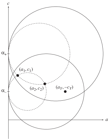
Figure 1: The circles $\bigcirc^{\mbox{\tiny HS}}_{\pm}$ surrounding $(a_{Y},-c_{Y})$ and the (dashed) circles $\bigcirc_{\pm}$ passing through $(a_{i},c_{i})$, for $i=1,2$, assuming $\alpha_{-}\leq\alpha_{+}$.

Remark 4.4.

The inequalities (4.19), (4.21) do not allow us to show that $c_{*}$ tends to zero when $c_{1}$ and $c_{2}$ approach zero, while keeping $a_{1}$, $a_{2}$, $b_{1}$, and $b_{2}$ fixed. To this end, we only have the bound (3.9) which reads as

$$|2\,c_{*}-c_{1}-c_{2}|\leq\frac{a_{*}}{\min\left(a_{1},a_{2}\right)}\,|c_{1}-c_{2}|.$$ (4.22)

Proof of Theorem 4.1. The proof is divided in four steps. In the first step we determine a suitable reference tensor $L_{0}$. In the second step we compute the tensor $\Gamma(\xi)$ involved in the $Y$-tensor approach. In the third step we compute the average $\langle\Gamma\rangle_{S^{2}}$. The fourth step is devoted to the derivation of the bounds.

First step : Determination of $L_{0}$.

Similarly to (2.7), let $L_{i}$, for $i=1,2,*$, be the symmetric tensor defined by

$$L_{i}:=\begin{pmatrix}(\sigma_{i}^{S})^{-1}&-\,(\sigma_{i}^{S})^{-1}\,\sigma_{i}^{A}\\ \vskip 6.0pt plus 2.0pt minus 2.0pt\cr\sigma_{i}^{A}\,(\sigma_{i}^{S})^{-1}&\sigma_{i}^{S}-\sigma_{i}^{A}\,(\sigma_{i}^{S})^{-1}\,\sigma_{i}^{A}\end{pmatrix}=\begin{pmatrix}\displaystyle{1\over a_{i}}&0&0&0&\displaystyle{c_{i}\over a_{i}}&0\\ 0&\displaystyle{1\over a_{i}}&0&\displaystyle-\,{c_{i}\over a_{i}}&0&0\\ 0&0&\displaystyle{1\over b_{i}}&0&0&0\\ 0&\displaystyle-\,{c_{i}\over a_{i}}&0&\displaystyle a_{i}+{c_{i}^{2}\over a_{i}}&0&0\\ \displaystyle{c_{i}\over a_{i}}&0&0&0&\displaystyle a_{i}+{c_{i}^{2}\over a_{i}}&0\\ 0&0&0&0&0&b_{i}\end{pmatrix}.$$ (4.23)

Now, let $L_{0}$ be the symmetric tensor defined by

$$L_{0}:=\begin{pmatrix}C_{1}&C_{2}\\ \vskip 6.0pt plus 2.0pt minus 2.0pt\cr C_{2}^{T}&C_{3}\end{pmatrix}=\begin{pmatrix}\displaystyle t_{1}&0&0&0&t_{2}&0\\ 0&t_{1}&0&-\,t_{2}&0&0\\ 0&0&t_{4}&0&0&0\\ 0&-\,t_{2}&0&t_{3}&0&0\\ t_{2}&0&0&0&t_{3}&0\\ 0&0&0&0&0&t_{5}\end{pmatrix},\quad\mbox{where }C_{j}\in\mathbb{R}^{3\times 3},\ C_{2}^{T}=-\,C_{2}.$$ (4.24)

The condition $L_{0}\geq 0$ is equivalent to

$$t_{1}\geq 0,\quad t_{4}\geq 0,\quad t_{3}\geq 0,\quad t_{5}\geq 0,\quad t_{1}t_{3}\geq t_{2}^{2}\,.$$ (4.25)

We also need $L_{i}\geq L_{0}$, which is equivalent to

$${1\over a_{i}}\geq t_{1},\quad\det\begin{pmatrix}\displaystyle{1\over a_{i}}-t_{1}&\displaystyle{c_{i}\over a_{i}}-t_{2}\\ \vskip 6.0pt plus 2.0pt minus 2.0pt\cr\displaystyle{c_{i}\over a_{i}}-t_{2}&\displaystyle a_{i}+{c_{i}^{2}\over a_{i}}-t_{3}\end{pmatrix}\geq 0,\quad\mbox{for }i=1,2,$$ (4.26)

$${1\over b_{i}}\geq t_{4},\quad b_{i}\geq t_{5},\quad\mbox{for }i=1,2.$$ (4.27)

From now on, assume that $b_{1}\geq b_{2}$, and set

$$t_{4}:={1\over b_{1}},\quad t_{5}=b_{2},$$ (4.28)

in order to make the inequalities (4.27) as sharp as possible.

On the other hand, the inequalities (4.26) show that the points $(a_{1},c_{1})$ and $(a_{2},c_{2})$ belong to the disk in the $a$-$c$ plane,

$$t_{1}\,(a^{2}+c^{2})+(t_{2}^{2}-t_{1}t_{3}-1)\,a-2t_{2}\,c+t_{3}\leq 0,$$ (4.29)

which lies in the half-plane $a\geq 0$. To make these bounds as tight as possible, we consider the two circles which are tangent to the $c$-axis, and which pass through the points $(a_{1},c_{1})$ and $(a_{2},c_{2})$. This requires

$$t_{3}={t_{2}^{2}\over t_{1}},$$ (4.30)

and the two circle equations

$$t_{1}^{2}\,(a_{i}^{2}+c_{i}^{2})-t_{1}\,a_{i}-2t_{1}t_{2}\,c_{i}+t_{2}^{2}=0,\quad\mbox{for }i=1,2,$$ (4.31)

which can be written as

$$\left\{\begin{array}[]{l}t_{1}^{2}\,a_{2}(a_{1}^{2}+c_{1}^{2})-t_{1}\,a_{1}a_{2}-2t_{1}t_{2}\,a_{2}c_{1}+t_{2}^{2}\,a_{2}=0\\ \vskip 6.0pt plus 2.0pt minus 2.0pt\cr t_{1}^{2}\,a_{1}(a_{2}^{2}+c_{2}^{2})-t_{1}\,a_{1}a_{2}-2t_{1}t_{2}\,a_{1}c_{2}+t_{2}^{2}\,a_{1}=0.\end{array}\right.$$ (4.32)

Subtracting and dividing by $t_{1}^{2}$, we get that $\alpha:=t_{2}/t_{1}$ solves

$$(a_{1}-a_{2})\,\alpha^{2}-2\,(a_{1}c_{2}-a_{2}c_{1})\,\alpha+a_{1}(a_{2}^{2}+c_{2}^{2})-a_{2}(a_{1}^{2}+c_{1}^{2})=0,$$ (4.33)

the discriminant of which is

$$(a_{1}c_{2}-a_{2}c_{1})^{2}+\left(a_{1}-a_{2}\right)\big{(}a_{2}(a_{1}^{2}+c_{1}^{2})-a_{1}(a_{2}^{2}+c_{2}^{2})\big{)}=a_{1}a_{2}\,\big{(}(a_{1}-a_{2})^{2}+(c_{1}-c_{2})^{2}\big{)}\geq 0.$$ (4.34)

Hence, equation (4.33) has two real solutions (one for each circle) $\alpha_{\pm}$ which are given by (4.15). Moreover, putting $t_{2}=\alpha\,t_{1}$ in (4.31) we obtain that

$$t_{1}={a_{i}\over a_{i}^{2}+(c_{i}-\alpha)^{2}}\leq{1\over a_{i}},\quad\mbox{for }i=1,2,$$ (4.35)

which implies that the ($2\times 2$) matrix in (4.26) is non-negative. Therefore, the choice of the coefficients $t_{1},t_{2},t_{3}$ given by

$$t_{1}={a_{1}\over a_{1}^{2}+(c_{1}-\alpha)^{2}},\quad t_{2}=\alpha\,t_{1},\quad t_{3}=\alpha^{2}\,t_{1},\quad\mbox{for }\alpha=\alpha_{\pm},$$ (4.36)

combined with (4.28), implies the desired inequalities $L_{i}\geq L_{0}$, for $i=1,2$. Making this choice in (4.29) the points $(a_{1},c_{1})$ and $(a_{2},c_{2})$ belong to the two circles of equation (4.20) which are tangent to the line $a=0$.

Second step : Computation of $\Gamma(\xi)$.

Let $\xi\in S^{2}$, $\xi=(\sin\theta\cos\varphi,\sin\theta\sin\varphi,\cos\theta)$. By virtue of Section 4.1 the tensor $\Gamma(\xi)$ is defined from the tensor $L_{0}$ (4.24), by

$$\begin{pmatrix}B_{1}\\ B_{2}\end{pmatrix}=\Gamma(\xi)\begin{pmatrix}A_{1}\\ A_{2}\end{pmatrix},\quad\mbox{for }A_{1},A_{2},B_{1},B_{2}\in\mathbb{R}^{3\times 3},$$ (4.37)

if and only if

$$\begin{pmatrix}I-\xi\otimes\xi&0\\ 0&\xi\otimes\xi\end{pmatrix}\begin{pmatrix}B_{1}\\ B_{2}\end{pmatrix}=\begin{pmatrix}B_{1}\\ B_{2}\end{pmatrix},$$ (4.38)

$$\mbox{and}\quad\begin{pmatrix}I-\xi\otimes\xi&0\\ 0&\xi\otimes\xi\end{pmatrix}\left[\begin{pmatrix}A_{1}\\ A_{2}\end{pmatrix}-\begin{pmatrix}C_{1}&C_{2}\\ C_{2}^{T}&C_{3}\end{pmatrix}\begin{pmatrix}B_{1}\\ B_{2}\end{pmatrix}\right]=0.$$ (4.39)

By (4.38) we have $B_{1}^{T}\xi=0$, and $B_{2}=\xi\otimes\eta$ for some vector $\eta$. From (4.39) it follows that

$$A_{2}^{T}\xi-B_{1}^{T}C_{2}\xi-B_{2}^{T}C_{3}^{T}\xi=A_{2}^{T}\xi-B_{1}^{T}C_{2}\xi-(C_{3}\xi\cdot\xi)\,\eta=0,$$ (4.40)

$$\begin{array}[]{ll}A_{1}-C_{1}B_{1}-C_{2}\,(\xi\otimes\eta)&=\xi\otimes\left(A_{1}^{T}\xi-B_{1}^{T}C_{1}^{T}\xi-B_{2}^{T}C_{2}^{T}\xi\right)\\ \vskip 6.0pt plus 2.0pt minus 2.0pt\cr&=\xi\otimes\left(A_{1}^{T}\xi-B_{1}^{T}C_{1}^{T}\xi-(C_{2}\xi\cdot\xi)\,\eta\right)\\ \vskip 6.0pt plus 2.0pt minus 2.0pt\cr&=\xi\otimes\left(A_{1}^{T}\xi-B_{1}^{T}C_{1}^{T}\xi\right)\quad\mbox{since }C_{2}^{T}=-\,C_{2},\\ \vskip 6.0pt plus 2.0pt minus 2.0pt\cr&=\xi\otimes k\quad\mbox{where }k:=A_{1}^{T}\xi-B_{1}^{T}C_{1}^{T}\xi.\end{array}$$ (4.41)

Noting that $C_{1}^{-1}C_{2}$ is antisymmetric, this implies that

$$0=B_{1}^{T}\xi=(C_{1}^{-1}A_{1})^{T}\xi-(\eta\otimes\xi)\,(C_{1}^{-1}C_{2})^{T}\xi-(k\otimes\xi)\,(C_{1}^{-1})^{T}\xi=(C_{1}^{-1}A_{1})^{T}\xi-(C_{1}^{-1}\xi\cdot\xi)\,k,$$ (4.42)

so we have

$$k={(C_{1}^{-1}A_{1})^{T}\xi\over C_{1}^{-1}\xi\cdot\xi}.$$ (4.43)

Moreover, replacing $B_{1}$ given by (4.41) in (4.40) and using that $(C_{1}^{-1})^{T}C_{2}$ is antisymmetric, we get that

$$\begin{array}[]{rl}0\kern-5.0pt&=A_{2}^{T}\xi-(C_{1}^{-1}A_{1})^{T}C_{2}\xi+(\eta\otimes\xi)\,(C_{1}^{-1}C_{2})^{T}C_{2}\xi+(k\otimes\xi)\,(C_{1}^{-1})^{T}C_{2}\xi-(\eta\otimes\xi)\,C_{3}^{T}\xi\\ \vskip 6.0pt plus 2.0pt minus 2.0pt\cr&=A_{2}^{T}\xi-(C_{1}^{-1}A_{1})^{T}C_{2}\xi-\left[(C_{3}-C_{2}^{T}C_{1}^{-1}C_{2})\,\xi\cdot\xi\right]\eta,\end{array}$$ (4.44)

hence

$$\eta={A_{2}^{T}\xi-(C_{2}^{T}C_{1}^{-1}A_{1})^{T}\xi\over D\xi\cdot\xi},\quad\mbox{where }D:=C_{3}-C_{2}^{T}C_{1}^{-1}C_{2}.$$ (4.45)

Again using (4.41) combined with (4.43) and (4.45) we deduce that

$$\begin{array}[]{rl}B_{1}=&\displaystyle C_{1}^{-1}A_{1}-{C_{1}^{-1}C_{2}\,(\xi\otimes\xi)\over D\xi\cdot\xi}\left(A_{2}-C_{2}^{T}C_{1}^{-1}A_{1}\right)-{C_{1}^{-1}\,(\xi\otimes\xi)\over C_{1}^{-1}\xi\cdot\xi}\,C_{1}^{-1}A_{1}\\ \vskip 6.0pt plus 2.0pt minus 2.0pt\cr B_{2}=&\displaystyle{\xi\otimes\xi\over D\xi\cdot\xi}\,A_{2}-{\xi\otimes\xi\over D\xi\cdot\xi}\,C_{2}^{T}C_{1}^{-1}A_{1}.\end{array}$$ (4.46)

Hence, from definition (4.37) it follows that

$$\Gamma(\xi)=\begin{pmatrix}\displaystyle C_{1}^{-1}+{C_{1}^{-1}C_{2}\,(\xi\otimes\xi)\,C_{2}^{T}C_{1}^{-1}\over D\xi\cdot\xi}-{C_{1}^{-1}\,(\xi\otimes\xi)\,C_{1}^{-1}\over C_{1}^{-1}\xi\cdot\xi}&&\displaystyle{C_{1}^{-1}C_{2}^{T}(\xi\otimes\xi)\over D\xi\cdot\xi}\\ \vskip 6.0pt plus 2.0pt minus 2.0pt\cr\displaystyle{(\xi\otimes\xi)\,C_{2}C_{1}^{-1}\over D\xi\cdot\xi}&&\displaystyle{\xi\otimes\xi\over D\xi\cdot\xi}\end{pmatrix}$$ (4.47)

which is a symmetric matrix since $C_{1}^{T}=C_{1}$ and $C_{2}^{T}=-\,C_{2}$.

Third step : Computation of $\left(\langle\Gamma\rangle_{S^{2}}\right)^{-1}$.

Note that the computation of $\Gamma(\xi)$ can be carried out if the matrix $D$ of (4.45)

$$D=\begin{pmatrix}d_{1}&0&0\\ 0&d_{1}&0\\ 0&0&d_{2}\end{pmatrix}=\begin{pmatrix}\displaystyle t_{3}-{t_{2}^{2}\over t_{1}}&0&0\\ 0&\displaystyle t_{3}-{t_{2}^{2}\over t_{1}}&0\\ 0&0&t_{5}\end{pmatrix},$$ (4.48)

is positive definite, i.e. $t_{1}t_{3}>t_{2}^{2}$ and $t_{5}>0$. Let us assume these conditions for the moment. We shall be able pass to the limit as $d_{1}\to 0$ in the expression of $\left(\langle\Gamma\rangle_{S^{2}}\right)^{-1}$. Set

$$P=\begin{pmatrix}p_{1}&0&0\\ 0&p_{1}&0\\ 0&0&p_{2}\end{pmatrix}:=\left\langle{\xi\otimes\xi\over D\xi\cdot\xi}\right\rangle_{S^{2}},$$ (4.49)

$$Q=\begin{pmatrix}q_{1}&0&0\\ 0&q_{1}&0\\ 0&0&q_{2}\end{pmatrix}:=\left\langle{\xi\otimes\xi\over C_{1}^{-1}\xi\cdot\xi}\right\rangle_{S^{2}},\quad R=\begin{pmatrix}r_{1}&0&0\\ 0&r_{1}&0\\ 0&0&r_{2}\end{pmatrix}:=C_{1}^{-1}-C_{1}^{-1}QC_{1}^{-1}.$$ (4.50)

By definition (1.6) we have

$$p_{1}=\left\langle{\xi_{1}^{2}\over d_{1}+(d_{2}-d_{1})\,\xi_{3}^{2}}\right\rangle_{S^{2}}\;\mathop{\longrightarrow}_{d_{1}\to 0}\;{1\over 4}\int_{0}^{\pi}{\sin^{3}\theta\over d_{2}\,\cos^{2}\theta}\,d\theta=\infty,$$ (4.51)

$$p_{2}=\left\langle{\xi_{3}^{2}\over d_{1}+(d_{2}-d_{1})\,\xi_{3}^{2}}\right\rangle_{S^{2}}\;\mathop{\longrightarrow}_{d_{1}\to 0}\;{1\over d_{2}}={1\over t_{5}}.$$ (4.52)

Moreover, the matrix

$$C_{1}^{-{1\over 2}}\,Q\,C_{1}^{-{1\over 2}}=\begin{pmatrix}\displaystyle{q_{1}\over t_{1}}&0&0\\ 0&\displaystyle{q_{1}\over t_{1}}&0\\ 0&0&\displaystyle{q_{2}\over t_{4}}\end{pmatrix}=\left\langle{C_{1}^{-{1\over 2}}\,(\xi\otimes\xi)\,C_{1}^{-{1\over 2}}\over C_{1}^{-1}\xi\cdot\xi}\right\rangle_{S^{2}}$$ (4.53)

has the property that its trace is $1$. This combined with definitions (1.6) and (4.14) yields

$$\left\{\begin{array}[]{rl}q_{2}=&\displaystyle t_{4}\left\langle{\xi_{3}^{2}\over(t_{4}/t_{1})(\xi_{1}^{2}+\xi_{2}^{2})+\xi_{3}^{2}}\right\rangle_{S^{2}}=t_{4}\,g(t_{1}/t_{4})\\ \vskip 6.0pt plus 2.0pt minus 2.0pt\cr q_{1}=&\displaystyle{t_{1}\over 2}\left(1-{q_{2}\over t_{4}}\right)={t_{1}\over 2}\big{(}1-g(t_{1}/t_{4})\big{)},\end{array}\right.$$ (4.54)

which also implies that

$$\left\{\begin{array}[]{rl}r_{1}=&\displaystyle{1\over t_{1}}-{q_{1}\over t_{1}^{2}}={1\over 2t_{1}}\big{(}1+g(t_{1}/t_{4})\big{)}\\ \vskip 6.0pt plus 2.0pt minus 2.0pt\cr r_{2}=&\displaystyle{1\over t_{4}}-{q_{2}\over t_{4}^{2}}={1\over t_{4}}\big{(}1-g(t_{1}/t_{4})\big{)}.\end{array}\right.$$ (4.55)

On the other hand, by definition (4.49) we have

$$C_{1}^{-1}C_{2}\,P\,C_{2}^{T}C_{1}^{-1}=\begin{pmatrix}\displaystyle{t_{2}^{2}\over t_{1}^{2}}\,p_{1}&0&0\\ 0&\displaystyle{t_{2}^{2}\over t_{1}^{2}}\,p_{1}&0\\ 0&0&0\end{pmatrix},\quad C_{1}^{-1}C_{2}^{T}P=\begin{pmatrix}\displaystyle 0&\displaystyle-\,{t_{2}\over t_{1}}\,p_{1}&0\\ \displaystyle{t_{2}\over t_{1}}\,p_{1}&0&0\\ 0&0&0\end{pmatrix}.$$ (4.56)

Then, putting (4.50) and (4.56) in the $S^{2}$-average of (4.47) we get that

$$\langle\Gamma\rangle_{S^{2}}=\begin{pmatrix}\displaystyle r_{1}+{t_{2}^{2}\over t_{1}^{2}}\,p_{1}&0&0&0&\displaystyle-\,{t_{2}\over t_{1}}\,p_{1}&0\\ 0&\displaystyle r_{1}+{t_{2}^{2}\over t_{1}^{2}}\,p_{1}&0&\displaystyle{t_{2}\over t_{1}}\,p_{1}&0&0\\ 0&0&r_{2}&0&0&0\\ 0&\displaystyle{t_{2}\over t_{1}}\,p_{1}&0&p_{1}&0&0\\ \displaystyle-{t_{2}\over t_{1}}\,p_{1}&0&0&0&p_{1}&0\\ 0&0&0&0&0&p_{2}\end{pmatrix},$$ (4.57)

which gives

$${1\over\langle\Gamma\rangle_{S^{2}}}=\begin{pmatrix}\displaystyle{1\over r_{1}}&0&0&0&\displaystyle{t_{2}\over t_{1}r_{1}}&0\\ 0&\displaystyle{1\over r_{1}}&0&\displaystyle-\,{t_{2}\over t_{1}r_{1}}&0&0\\ 0&0&\displaystyle{1\over r_{2}}&0&0&0\\ 0&\displaystyle-\,{t_{2}\over t_{1}r_{1}}&0&\displaystyle{1\over p_{1}}+{t_{2}^{2}\over t_{1}^{2}\,r_{1}}&0&0\\ \displaystyle{t_{2}\over t_{1}r_{1}}&0&0&0&\displaystyle{1\over p_{1}}+{t_{2}^{2}\over t_{1}^{2}\,r_{1}}&0\\ 0&0&0&0&0&\displaystyle{1\over p_{2}}\end{pmatrix}$$ (4.58)

Therefore, passing to the limit as $d_{1}\to 0$, or equivalently $t_{3}\to t_{2}^{2}/t_{1}$, (4.51) and (4.52) imply that

$${1\over\langle\Gamma\rangle_{S^{2}}}=\begin{pmatrix}\displaystyle{1\over r_{1}}&0&0&0&\displaystyle{t_{2}\over t_{1}r_{1}}&0\\ 0&\displaystyle{1\over r_{1}}&0&\displaystyle-\,{t_{2}\over t_{1}r_{1}}&0&0\\ 0&0&\displaystyle{1\over r_{2}}&0&0&0\\ 0&\displaystyle-\,{t_{2}\over t_{1}r_{1}}&0&\displaystyle{t_{2}^{2}\over t_{1}^{2}\,r_{1}}&0&0\\ \displaystyle{t_{2}\over t_{1}r_{1}}&0&0&0&\displaystyle{t_{2}^{2}\over t_{1}^{2}\,r_{1}}&0\\ 0&0&0&0&0&\displaystyle t_{5}\end{pmatrix}.$$ (4.59)

Fourth step : Derivation of the bounds.

On the one hand, the Appendix of [21] (see also formula (19.3) of [26]) yields the following formula for the $Y$-tensor defined by (4.2)

$$Y_{*}=-f_{2}\,\sigma_{1}-f_{1}\,\sigma_{2}+f_{1}f_{2}\left(\sigma_{1}-\sigma_{2}\right)\left(f_{1}\,\sigma_{1}+f_{2}\,\sigma_{2}-\sigma_{*}\right)^{-1}\left(\sigma_{1}-\sigma_{2}\right).$$ (4.60)

Note that, due to the transverse isotropy of $\sigma_{i}$, for $i=1,2,*$, we have

$$Y_{*}=\begin{pmatrix}a_{Y}&-c_{Y}&0\\ c_{Y}&a_{Y}&0\\ 0&0&b_{Y}\end{pmatrix}.$$ (4.61)

This relation also separates into blocks, so that we obtain for the ₃₃ entry of $Y_{*}$ the relation (4.18). Moreover, making the correspondence

$$\begin{pmatrix}a&-c\\ c&a\end{pmatrix}\;\longleftrightarrow\,a+i\,c,$$ (4.62)

we deduce from the first $(2\times 2)$ block of (4.60) the relation (4.17).

On the other hand, by (4.61) the formula (4.5) for $\mathcal{Y}^{*}$ reads as

$$\mathcal{Y}_{*}=\begin{pmatrix}\displaystyle{1\over a_{Y}}&0&0&0&\displaystyle-\,{c_{Y}\over a_{Y}}&0\\ 0&\displaystyle{1\over a_{Y}}&0&\displaystyle{c_{Y}\over a_{Y}}&0&0\\ 0&0&\displaystyle{1\over b_{Y}}&0&0&0\\ 0&\displaystyle{c_{Y}\over a_{Y}}&0&\displaystyle a_{Y}+{c_{Y}^{2}\over a_{Y}}&0&0\\ \displaystyle-\,{c_{Y}\over a_{Y}}&0&0&0&\displaystyle a_{Y}+{c_{Y}^{2}\over a_{Y}}&0\\ 0&0&0&0&0&b_{Y}\end{pmatrix}.$$ (4.63)

Then, the bound (4.11) applied with the formulas (4.63) for $\mathcal{Y}_{*}$, (4.24) for $L_{0}$ and (4.59) for $\left(\langle\Gamma\rangle_{S^{2}}\right)^{-1}$, combined with (4.28), (4.54), and (4.55), implies that

$${1\over b_{Y}}+{1\over b_{1}}\geq{1\over r_{2}}={1\over b_{1}\big{(}1-\displaystyle g(b_{1}t_{1})\big{)}},\quad b_{Y}\geq 0,$$ (4.64)

and

$$\det\begin{pmatrix}\displaystyle{1\over a_{Y}}-s_{1}&\displaystyle{c_{Y}\over a_{Y}}+s_{2}\\ \vskip 6.0pt plus 2.0pt minus 2.0pt\cr\displaystyle{c_{Y}\over a_{Y}}+s_{2}&\displaystyle a_{Y}+{c_{Y}^{2}\over a_{Y}}-s_{3}\end{pmatrix}\geq 0,$$ (4.65)

where

$$\left\{\begin{array}[]{rll}s_{1}:=&\displaystyle{1\over r_{1}}-t_{1}&\displaystyle=t_{1}\left({2\over 1+\displaystyle g(b_{1}t_{1})}-1\right)\geq 0\quad(\mbox{since }0<g(b_{1}t_{1})<1)\\ \vskip 6.0pt plus 2.0pt minus 2.0pt\cr s_{2}:=&\displaystyle{t_{2}\over t_{1}r_{1}}-t_{2}&\displaystyle=t_{2}\left({2\over 1+\displaystyle g(b_{1}t_{1})}-1\right)\\ \vskip 6.0pt plus 2.0pt minus 2.0pt\cr s_{3}:=&\displaystyle{t_{2}^{2}\over t_{1}^{2}r_{1}}-t_{3}.\end{array}\right.$$ (4.66)

Due to (4.30) we have $s_{1}s_{3}=s_{2}^{2}$. Therefore, similarly to (4.26) and (4.29) the inequality (4.65) can be written as

$$a_{Y}^{2}+\left(c_{Y}+{s_{2}\over s_{1}}\right)^{2}-{a_{Y}\over s_{1}}\leq 0.$$ (4.67)

Finally, taking into account (4.16), (4.36), (4.66) the inequalities (4.67) and (4.64) correspond respectively to the desired bounds (4.19), (4.21). Theorem 4.1 is proved. $\hfill\Box$

Acknowledgements. GWM is grateful for support from the Mathematical Sciences Research Institute and from National Science Foundation through grant DMS-0707978.

References

- [1] G. Alessandrini and V. Nesi, Univalent -harmonic mappings, Arch. Ratio. Mech. Anal., 158 (2001), pp. 155–171.
- [2] G. Alessandrini and V. Nesi, Beltrami operators, non-symmetric elliptic equations and quantitative Jacobian bounds, Ann. Acad. Sci. Fenn. Math., 34 (2009), pp. 47–67.
- [3] G. Allaire, Shape Optimization by the Homogenization Method, Appl. Math. Sci. 146, Springer-Verlag, New York, 2002.
- [4] A. Bensoussan, J. L. Lions, and G. Papanicolaou, Asymptotic Analysis for Periodic Structures, North-Holland, Amsterdam, New York, 1978.
- [5] D. J. Bergman, Self-duality and the low field Hall effect in 2D and 3D metal-insulator composites, in Percolation Structures and Processes, Annals of the Israel Physical Society, Vol. 5, G. Deutscher, R. Zallen, and J. Adler, eds., Israel Physical Society, Jerusalem, 1983, pp. 297–321.
- [6] D. J. Bergman, X. Li, and Y. M. Strelniker, Macroscopic conductivity tensor of a three-dimensional composite with a one- or two-dimensional microstructure, Phys. Rev. B, 71 (2005), 035120.
- [7] D. J. Bergman and Y. M. Strelniker, Duality transformation in a three dimensional conducting medium with two dimensional heterogeneity and an in-plane magnetic field, Phys. Rev. Lett., 80 (1998), pp. 3356–3359.
- [8] D. J. Bergman and Y. M. Strelniker, Strong-field magnetotransport of conducting composites with a columnar microstructure, Phys. Rev. B, 59 (1999), pp. 2180–2198.
- [9] D. J. Bergman and Y. M. Strelniker, Magnetotransport in conducting composite films with a disordered columnar microstructure and an in-plane magnetic field, Phys. Rev. B, 60 (1999), pp. 13016–13027.
- [10] D. J. Bergman, Y. M. Strelniker, and A. K. Sarychev, Recent advances in strong field magneto-transport in a composite medium, Phys. A, 241 (1997), pp. 278–283.
- [11] J. G. Berryman, Effective medium theory for elastic composites. In V. K. Varadan and V. V. Varadan (eds.), Elastic Waves Scattering and Propagation: Based on Presentations made at a Special Session of the Midwestern Mechanics Conference Held at the University of Michigan, Ann Arbor, Michigan: Ann Harbor Science, May 7-9, 1981, pp. 111-129.
- [12] M. Briane, Corrector for the homogenization of a laminate, Adv. Math. Sci. Appl., 4 (1994), pp. 357–379.
- [13] M. Briane and G. W. Milton, Homogenization of the three-dimensional Hall effect and change of sign of the Hall coefficient, Arch. Ratio. Mech. Anal., 193 (2009), pp. 715–736.
- [14] M. Briane and G. W. Milton, Giant Hall effect in composites, Multiscale Model. Simul., 7 (2009), pp. 1405–1427.
- [15] M. Briane and G. W. Milton, New bounds on strong field magneto-transport in multiphase columnar composites, SIAM J. Appl. Math., 70 (8), 3272-3286 (2010).
- [16] M. Briane, D. Manceau and G. W. Milton, Homogenization of the two-dimensional Hall effect, J. Math. Anal. Appl., 339 (2008), 1468–1484.
- [17] A. V. Cherkaev and L. V. Gibiansky, Variational principles for complex conductivity, viscoelasticity, and similar problems in media with complex moduli, J. Math. Phys., 35 (1994), pp. 127–145.
- [18] A. Fannjiang and G. Papanicolaou, Convection enhanced diffusion for periodic flows, SIAM J. Appl. Math., 54 (1994), pp. 333–408.
- [19] E. H. Hall, On a new action of the magnet on electric currents, Amer. J. Math., 2 (3) (1879), 287–292.
- [20] Z. Hashin and S. Shtrikman, A variational approach to the theory of the effective magnetic permeability of multiphase materials, J. Appl. Phys., 35 (1962), 3125–3131.
- [21] L. V. Gibiansky and G. W. Milton, On the effective viscoelastic moduli of two-phase media. I. Rigorous bounds on the complex bulk modulus., Proc. Roy. Soc. London. Ser. A, Math. Phys. Sci., 440 (1908), pp. 163–188.
- [22] Y. Grabovsky, An application of the general theory of exact relations to fiber-reinforced conducting composites with Hall effect, Mech. Mater., 41 (2009), pp. 456–462.
- [23] Y. Grabovsky, Exact relations for effective conductivity of fiber-reinforced conducting composites with the Hall effect via a general theory, SIAM J. Math. Anal., 41 (2009), pp. 973–1024.
- [24] G. W. Milton, Classical Hall effect in two-dimensional composites: A characterization of the set of realizable effective conductivity tensors, Phys. Rev. B, 38 (1988), pp. 11296–11303.
- [25] G. W. Milton, On characterizing the set of possible effective tensors of composites: The variational method and the translation method, Comm. Pure Appl. Math., 43 (1990), pp. 63–125.
- [26] G. W. Milton, The Theory of Composites, Cambridge University Press, Cambridge, UK, 2002.
- [27] G. W. Milton, Modelling the properties of composites by laminates, in Homogenization and Effective Moduli of Materials and Media, IMA Vol. Math Appl., 1, Springer-Verlag, New York, 1986, pp. 150.
- [28] G. W. Milton, Bounds on the electromagnetic, elastic, and other properties of two-component composites. Phys. Review Letters, 46 (8), 1981, pp. 542-545.
- [29] F. Murat, -convergence, mimeographed notes, Séminaire d’Analyse Fonctionnelle et Numérique, Université d’Alger, Algiers, 1978 (English translation in [30]).
- [30] F. Murat and L. Tartar, -convergence, in Topics in the Mathematical Modelling of Composite Materials, Progr. Nonlinear Differential Equations Appl. 31, L. Cherkaev and R. V. Kohn, eds., Birkhaüser Boston, Boston, 1997, pp. 21–43.
- [31] Y. M. Strelniker and D. J. Bergman, Exact relations between magnetoresistivity tensor components of conducting composites with a columnar microstructure, Phys. Rev. B, 61 (2000), pp. 6288–6297.
- [32] D. Stroud and D. J. Bergman, New exact results for the Hall-coefficient and magnetoresistance of inhomogeneous two-dimensional metals, Phys. Rev. B, 30 (1984), pp. 447–449.
- [33] L. Tartar, Cours Peccot, Collège de France, Paris, 1977, unpublished (partly written in [29, 30]).
- [34] J. R. Willis, Bounds and self-consistent estimates for the overall properties of anisotropic composites, J. Mech. Phys. Solids, 25 (3) (1977), pp. 185–202.