A cosmic speed-trap: a gravity-independent test of cosmic acceleration using baryon acoustic oscillations

Abstract

We propose a new and highly model-independent test of cosmic acceleration by comparing observations of the baryon acoustic oscillation (BAO) scale at low and intermediate redshifts: we derive a new inequality relating BAO observables at two distinct redshifts, which must be satisfied for any reasonable homogeneous non-accelerating model, but is violated by models similar to $\Lambda$CDM, due to acceleration in the recent past. This test is fully independent of the theory of gravity (GR or otherwise), the Friedmann equations, CMB and supernova observations: the test assumes only the Cosmological Principle, and that the length-scale of the BAO feature is fixed in comoving coordinates. Given realistic medium-term observations from BOSS, this test is expected to exclude all homogeneous non-accelerating models at $\sim 4\sigma$ significance, and can reach $\mathrel{\lower 2.58334pt\hbox{$\buildrel{\textstyle>}\over{\scriptstyle\sim}$}}7\sigma$ with next-generation surveys.

1 Introduction

In the last 10–15 years, the $\Lambda$CDM model has been established as the standard model of large-scale cosmology; the model is an excellent match to many observations including the anisotropies in the CMB measured by WMAP (Komatsu et al, 2011) and other experiments, the large-scale clustering of galaxies (Percival et al, 2010), the Hubble diagram for high-z supernovae (Guy et al, 2010; Conley et al, 2011), and the abundance and baryon fraction of rich clusters of galaxies (Allen et al, 2011).

Despite these great observational successes, the model appears unnatural since 96% of the universe’s mass-energy is not observed, but is only inferred from fitting the observations. Also, the dark sector contains at least two apparently unrelated components, dark matter and dark energy; recent reviews of dark energy are given by Frieman, Turner & Huterer (2008) and Linder (2008).

The most direct evidence for cosmic acceleration comes from the Hubble diagram of Type-Ia supernovae (Guy et al, 2010; Conley et al, 2011), which shows that SNe at $0.3\mathrel{\lower 2.58334pt\hbox{$\buildrel{\textstyle<}\over{\scriptstyle\sim}$}}z\mathrel{\lower 2.58334pt\hbox{$\buildrel{\textstyle<}\over{\scriptstyle\sim}$}}0.9$ are fainter, relative to local SNe, than can be accommodated in any Friedmann-Robertson-Walker model without dark energy. A model-independent approach has also been given by Shapiro & Turner (2006), who show that the SNe results require accelerated expansion at $z<0.4$ at around the $5\sigma$ significance level without assuming the Friedmann equations.

However, there are some possible loopholes in the supernova results: since they are fundamentally based on brightness measurements, the interpretation could be affected by either unexpected evolution of the mean SNe properties over cosmic time, or some process which removes photons en route to our telescopes, such as peculiar dust or more exotic effects such as photon-dark matter interactions. The simplest such effects with monotonic time-dependence are strongly disfavoured by SN observations at $z>1$ (Riess et al, 2007), but more complex time-dependent effects could still leave these loopholes open.

Independent of supernovae, there is powerful support for dark energy from observations of the anisotropies in the cosmic microwave background (Larson et al, 2010; Komatsu et al, 2011) and the large-scale clustering of galaxies (Percival et al, 2010), but this is dependent on assuming general relativity and the Friedmann equations; if these both hold, the model parameters are tightly constrained by CMB and LSS data, and the expansion history $a(t)$ must match $\Lambda$CDM models within a few percent. However, in alternative gravity theories, we cannot make model-independent statements from the CMB or large-scale structure: clearly any successful modified-gravity model should eventually be consistent with these observations, but the model space of modified gravity is large and the calculations non-trivial; so in non-GR models we cannot necessarily use the CMB and LSS observations to make any definite statement about recent acceleration.

The accelerated expansion is so startling that it is desirable to test it via multiple routes with a minimum number of model assumptions. A very direct test of acceleration has been proposed using the “cosmic drift”, which is the small change in redshift for fixed object(s) over time (e.g. Liske et al 2008); the predicted change is $dz/dt=(1+z)H_{0}-H(z)$. However, this effect is tiny over human timescales, of order cm/s/year, and will probably require over 20 years baseline to get a convincing detection.

Here we propose a new and robust test for cosmic acceleration based only on the cosmic “standard ruler” in the galaxy correlation function: in the standard model, this is a feature created by acoustic oscillations in the baryon-photon fluid before recombination (e.g. Peebles & Yu 1970); this was analysed in more detail by Eistenstein & Hu (1998) and Meiksin, White & Peacock (1999), then first detected in 2005 by Eisenstein et al (2005) in SDSS data, and Cole et al (2005) using the 2dFGRS survey. The length of this ruler, hereafter $r_{s}$, depends only on matter and radiation densities and is accurately predicted from CMB observations at $\approx 153\pm 2\,{\rm Mpc}$ (Komatsu et al, 2011). Many recent studies (e.g. Eisenstein, Seo & White 2007, Shoji, Jeong & Komatsu 2009, Abdalla et al 2010, Tian et al 2011) have shown how precision measurements of this BAO scale from huge galaxy redshift surveys can provide powerful constraints on the properties of dark energy, and test for evolution of dark energy density; more details are given in Section 2.

However, in the current paper we do not assume any gravity theory or the actual length scale of this feature, only that we can observe some feature at a specific lengthscale imprinted on the galaxy distribution at high redshift, which expands with the Hubble expansion and remains a constant ruler in comoving coordinates. We then derive an inequality relating observations comparing this ruler at low and intermediate redshift, which is satisfied in any reasonable non-accelerating model, but is violated by accelerating models approximating $\Lambda$CDM. In more detail, we use the radial component of the BAO feature at $z_{2}\sim 0.75$ to constrain the product $H(z_{2})\,r_{s}$, and we then compare to the spherical-averaged BAO feature at low redshift $z_{1}\sim 0.2$, which is related to the average of $1/H(z)$ at $0\leq z\leq z_{1}$. Then, assuming any non-accelerating model we derive a strict upper limit on the ratio of these. Models approximating standard $\Lambda$CDM predict a result which violates this inequality by a substantial amount $\sim 10-20\%$, depending on cosmological parameters and redshift. Future large redshift surveys should be able to measure this ratio to $\leq 2\%$ precision: assuming our inequality is significantly violated as predicted, we can then exclude all homogeneous non-accelerating models regardless of Friedmann equations, gravity theory or details of the expansion history.

The plan of the paper is as follows: in § 2 we review the basic features and observables of baryon acoustic oscillations. In § 3 we derive the new inequality relating BAO observables for non-accelerating models. In § 4 we discuss future observations and related issues, and we summarise our conclusions in § 5.

2 Observations of the BAO feature

The baryon acoustic oscillation (hereafter BAO) feature (Eistenstein & Hu, 1998; Meiksin, White & Peacock, 1999) is a bump in the galaxy correlation function $\xi(r)$, or equivalently a decaying series of wiggles in the power spectrum $P(k)$, corresponding to a comoving length denoted by $r_{s}$, created by acoustic waves in the early universe prior to decoupling. (See Bassett & Hlozek (2010) for a recent review). In the standard model, its length-scale is essentially set by the distance that a sound wave can propagate prior to the “drag epoch” at $z_{d}\approx 1020$, denoted $r_{s}(z_{d})$, and this length depends only on physical densities of matter $\Omega_{m}h^{2}$ and baryons $\Omega_{b}h^{2}$, (together with radiation density $\Omega_{r}h^{2}$ which is pinned very precisely by the CMB temperature). In the standard model the relative heights of the acoustic peaks in CMB anisotropies constrain $\Omega_{m}h^{2}$ and $\Omega_{b}h^{2}$ well (Komatsu et al, 2011), which leads to a prediction $r_{s}\approx 153\,{\rm Mpc}$ comoving with approximately 1.5 percent precision. This predicted length does not rely on the assumption of a flat universe, since the relative CMB peak heights constrain the various densities reasonably well without assuming flatness. However, the CMB-predicted length $r_{S}$ does depend on assuming standard GR, and several assumptions about the mass-energy budget including standard neutrino content, negligible early dark energy, no late-decaying dark matter, negligible admixture of isocurvature perturbations, etc. However, in the rest of this paper we leave $r_{s}$ as an arbitrary comoving scale, which cancels later.

The BAO feature provides a standard ruler which can be observed at low to moderate redshift using very large galaxy redshift surveys; in the small angle approximation and assuming we observe a redshift shell which is thin compared with its mean redshift $z$, there are two primary observables derived from a BAO survey: firstly the angle on the sky subtended by the BAO feature transverse to the line of sight, $\Delta\theta(z)=r_{s}/[(1+z)D_{A}(z)]$, where $D_{A}(z)$ is the conventional (proper) angular-diameter distance to redshift $z$; and secondly the difference in redshift along one BAO length along the line of sight is $\Delta z_{/\!/}(z)=r_{s}H(z)/c$ (e.g. Blake & Glazebrook 2003, Seo & Eisenstein 2003). We note that calculating comoving galaxy separations from observed positions and redshifts requires a reference cosmology, hence a difference between the true and reference cosmology will produce an error in the inferred $r_{s}$; however, any error in the reference model cancels to first order in the dimensionless ratios $r_{s}/D_{A}(z)$ and $r_{s}\,H(z)/c$, so both of these ratios can be well constrained with minimal theory-dependence by measuring BAOs in a galaxy redshift survey.

The ability to independently probe $D_{A}(z)$ and $H(z)$ is a powerful advantage of BAOs over other low-redshift cosmological tests. Furthermore, a redshift survey useful for BAOs can also measure growth of structure via redshift-space distortions and thus test for consistency with GR, though we do not consider this here.

However, in practice, current galaxy redshift surveys are not quite large enough to robustly measure the BAO feature separately in angular and radial directions (though there are tentative detections, e.g. Gaztanaga et al 2009 ). The current measurements primarily constrain a spherically-averaged scale, called $D_{V}$, which is defined by Eisenstein et al (2005) as

$$D_{V}(z)\equiv\left[(1+z)^{2}D_{A}^{2}(z)\frac{cz}{H(z)}\right]^{1/3}\ ;$$ (1)

this is essentially a geometric mean of two transverse directions and one radial direction. Observations using the 2dFGRS and SDSS-II redshift surveys have measured the dimensionless ratio $d(z)\equiv r_{s}/D_{V}(z)$ at low redshifts (Percival et al, 2010; Kazin et al, 2010), which we discuss later. We note that as $z\rightarrow 0$, $D_{V}(z)\rightarrow cz/H_{0}$; however, this approximation is not very useful in practice, since we cannot measure the BAO feature at very low redshift $z<0.02$ where corrections of order $z^{2}$ are unimportant. We give a better approximation below in § 4.2.

In practice, the BAO feature is not a sharp spike but a hump in $\xi(r)$ of width approximately 15% of $r_{s}$, so there are several subtle effects in actually extracting the scale $r_{s}$ from a redshift survey: we discuss these in more detail in § 4.1. However, for the purposes of this paper we only need to assume that $r_{s}$ is a constant comoving length to $\sim 1\%$ at redshift $\leq 0.8$, so these precision details are relatively unimportant for the rest of this paper.

3 The cosmic speed trap

Here we derive a new inequality which we denote the “cosmic speed-trap”, which must be satisfied by any reasonable non-accelerating model, but is violated by $\Lambda$CDM and other accelerating models. We start off by assuming an arbitrary non-accelerating model, and deriving a lower limit for $D_{V}(z_{1})$ in terms of the value of $H(z_{2})$ at a higher redshift $z_{2}$. Then, we form a ratio of BAO observables which eliminates $H(z_{2})$ and $r_{s}$, and we obtain the speed-trap inequality (14) which forms our main new result.

3.1 An inequality for $D_{V}$ in non-accelerating models

Here we derive an inequality for $D_{V}(z)$ which is satisfied in any non-accelerating model, but may be violated by acceleration.

First we define as usual $a$ to be the cosmic expansion factor relative to the present day with $a_{0}=1$, redshift $z$ by $1+z\equiv a^{-1}$, and the Hubble parameter $H(a)=\dot{a}/a$ where dot represents time derivative. Then we have the expansion rate

$$\dot{a}=aH(a)=\frac{H(z)}{1+z}\ ;$$ (2)

if the expansion of the universe was non-accelerating, then $\ddot{a}$ is non-positive and the function above must be non-increasing with time or $a$, therefore non-decreasing with increasing $z$. Therefore, if we consider any two redshifts $z_{1}<z_{2}$, in any non-accelerating universe,

$$\frac{H(z_{1})}{1+z_{1}}\leq\frac{H(z_{2})}{1+z_{2}}\ .$$ (3)

Assuming only the cosmological principle, any observed violation of this inequality is a direct proof that the expansion has accelerated, on average, between the earlier epoch $z_{2}$ and the later epoch $z_{1}$, without reference to any specific theory of gravity or geometry.

A concordance $\Lambda$CDM model does violate this inequality due to the recent positive acceleration: a minimum value of $H(z)/(1+z)$ occurred at $z_{\rm acc}=\sqrt[3]{2\,\Omega_{\Lambda}/\Omega_{m}}-1$; for the concordance value $\Omega_{m}\approx 0.27$, this gives $z_{\rm acc}\approx 0.75$, and $H(z_{\rm acc})/(1+z_{\rm acc})\approx 0.85\,H_{0}$. The expansion rate $H(z)/(1+z)$ is shown in Figure 1 for a few representative models: it is notable that the value of $H(z)/(1+z)$ remains within a few percent of its minimum between $0.5\leq z\leq 1.2$, and it rises rather sharply at low redshift; for the concordance model it only crosses the half-way value between the minimum and the present-day $H_{0}$ at the modest redshift of $z\approx 0.17$, and three-quarters of the speedup has occurred since $z\approx 0.31$. Thus the actual speedup of the expansion rate is quite concentrated at rather low redshift; this becomes relevant later.

Figure 1: The expansion rate $\dot{a}=H(z)/(1+z)$ from the standard Friedmann equation is shown as a function of redshift, for four models: three flat $\Lambda$CDM with respectively $\Omega_{m}=0.24$ (dashed), 0.27 (solid) and 0.31 (dot-dash); also one wCDM model with $\Omega_{m}=0.32$, $w=-0.85$ (dotted). The upper panel shows expansion rate relative to present-day $H_{0}$, while the lower panel shows absolute expansion rate, where for each model $H_{0}$ is adjusted to keep the CMB acoustic angle constant. Parameters are given in Table 1.

Model	$\Omega_{m}$	$H_{0}$	$w$	$t_{0}$
		($\,{\rm km\,s^{-1}\,Mpc^{-1}}$)		(Gyr)
C	0.27	70.0	$-1$	13.86
L	0.24	72.5	$-1$	13.82
H	0.31	67.1	$-1$	13.91
W	0.32	64.6	$-0.85$	13.98

Table 1: Cosmological parameters for the four example models discussed in the text; model C is the baseline concordance model, while the others are selected to roughly span the current $2\sigma$ allowed range in $\Omega_{m}$ and $w$. All are flat, and have $H_{0}$ adjusted to give very similar values of $\ell_{A}$ consistent with WMAP, therefore have similar values of $t_{0}$.

Next, we suppose we have a measurement of $H(z_{2})$ at an earlier epoch $z_{2}$; for a non-accelerating model we now derive a lower limit on $D_{V}(z_{1})$ at a later epoch $z_{1}$ where $z_{1}<z_{2}$.

The comoving radial distance to redshift $z_{1}$ is

$$D_{R}(z_{1})=c\int_{0}^{z_{1}}\frac{1}{H(z)}\,dz\quad.$$ (4)

If the universe is non-accelerating and $z_{1}<z_{2}$, we can rearrange inequality (3) into $1/H(z)\geq(1+z_{2})/[H(z_{2})(1+z)]$; inserting this we have

$$D_{R}(z_{1})\geq{c\,(1+z_{2})\over H(z_{2})}\ln(1+z_{1})$$ (5)

The proper angular-diameter distance $D_{A}(z)$ is defined by

$$(1+z)D_{A}(z)\equiv|R_{C}|\,S_{k}\left({D_{R}(z)\over|R_{C}|}\right)=D_{R}(z){S_{k}(x)\over x}$$ (6)

where $|R_{C}|$ is the curvature radius of the universe in comoving Mpc, $x\equiv D_{R}(z)/|R_{C}|$, and the function $S_{k}(x)$ = $\sinh x,\ x,\ \sin x$ for the cases $k=-1,\,0,\,+1$ where $k$ is the sign of the curvature.

Note that in the above we have left $R_{C}$ as a constant but arbitrary curvature radius, thus we have not assumed the Friedmann equation which gives $R_{C}=(c/H_{0})\sqrt{k/(\Omega_{tot}-1)}$; we have only assumed that the universe has a metric with some well-defined curvature radius $R_{C}$, which follows from the assumption of homogeneity and isotropy (Peacock, 1999). Also, we have not assumed any functional form for $H(z)$, only that it obeys the non-acceleration condition (3) at all $z\leq z_{2}$; what happened earlier at $z\geq z_{2}$ is immaterial.

For the other term in $D_{V}$, we use a similar inequality for $1/H(z_{1})$ as above, which is

$${cz_{1}\over H(z_{1})}\geq{cz_{1}(1+z_{2})\over H(z_{2})(1+z_{1})}\ ;$$ (7)

substituting both of the above into Eq. 1, we obtain the inequality

$$D_{V}(z_{1})\geq{c(1+z_{2})\over H(z_{2})}\left[z_{1}\,(\ln(1+z_{1}))^{2}\over 1+z_{1}\right]^{1/3}\,\left({S_{k}(x_{1})\over x_{1}}\right)^{2/3}\;.$$ (8)

where $x_{1}\equiv D_{R}(z_{1})/|R_{C}|$ as above.

This inequality is strict for any non-accelerating and homogeneous universe with a Robertson-Walker metric, independent of details of the expansion history or the gravity model. This is not so useful on its own, but we will see in the next section how to combine observables to cancel the $z_{2}$ dependence.

We note that the factor $(S_{k}(x_{1})/x_{1})^{2/3}=1$ exactly for flat models, and is $\geq 1$ for open models (so open models always strengthen the inequality); the factor is $\leq 1$ for closed models which weakens our inequality, but only by a small amount if we consider sufficiently low redshift $z_{1}$, since the effect of curvature on distances only enters to third order in $z$; at small $x$ and $k=+1$ we have

$$\left({S_{k}(x)\over x}\right)^{2/3}\approx 1-\frac{x^{2}}{9}$$

therefore we need an upper limit on $x$ for closed models. We get a firm limit as follows, using an upper bound on $D_{R}$ and a lower bound on $R_{C}$ for closed models.

To limit $D_{R}$, we can use the non-acceleration inequality (3) between $z=0$ and an upper redshift $z_{1}$ to get $1/H(z)\leq 1/[H_{0}(1+z)]$, which now leads to an upper bound on $D_{R}(z_{1})$ in terms of $H_{0}$, $D_{R}(z_{1})\leq(c/H_{0})\ln(1+z_{1})\leq cz_{1}/H_{0}$, for any non-accelerating model. This gives $x_{1}\leq cz_{1}/H_{0}R_{C}$.

We may also obtain a lower bound on $R_{C}$ as follows: in a closed model, it is clear from Eq. 6 and $\sin x\leq 1$ that $D_{A}(z)$ cannot exceed $R_{C}/(1+z)$ regardless of the expansion history $H(z)$. If we take for example $R_{C}=0.6\,c/H_{0}$ and $H_{0}=70\,{\rm km\,s^{-1}\,Mpc^{-1}}$, this leads to $D_{A}(z=3)\leq 642\,{\rm Mpc}$, only $0.4\times$ the concordance value of $1638\,{\rm Mpc}$. However, observed angular sizes of $z\sim 3$ galaxies already convert to rather small physical sizes based on the concordance model, and making them smaller by another factor $<0.4$ appears to be seriously discrepant. We therefore exclude closed models with $R_{C}<0.6\,c/H_{0}$.

A stronger lower bound may be obtained with other methods: e.g. the luminosity distance $D_{L}(z=1.5)$ measured from SNe (Riess et al, 2007) agrees well with the concordance model, and if we adopt a lower bound $0.8\times$ the concordance value, we obtain $R_{C}\geq 0.84\,c/H_{0}$. However, to remain fully independent of SNe data we do not use this below. A stronger limit should also be possible in future using angular BAO measurements at $z\sim 3$, e.g. from the HETDEX or BOSS projects.

However, for the following we take $R_{C}\geq 0.6\,c/H_{0}$ as a conservative gravity-independent lower limit for closed models. This leads to a firm upper limit $x\leq\ln(1+z)/0.6$ for closed non-accelerating models, which we use below.

3.2 The observable speed-trap

The above inequality (8) relates the volume-distance $D_{V}(z_{1})$ at low redshift to the Hubble constant $H(z_{2})$ at a higher redshift. Neither of these quantities are directly observable at present, but it is possible to measure both of them relative to the BAO length-scale $r_{s}$; then, dividing these two cancels the length scale $r_{s}$ and gives a ratio measurement. Applying the $D_{V}$ inequality above gives us a limit which must be satisfied by any reasonable non-accelerating model, but is found to be violated by an expansion history close to $\Lambda$CDM, for a range of suitable choices of $z_{1}\sim 0.2,\;z_{2}\sim 0.75$.

The Hubble parameter $H(z_{2})$ may be measured using the radial BAO scale (along the line of sight) in a redshift shell near $z_{2}$; for a thin shell and ignoring redshift-space distortion effects, this gives the observable

$$\Delta z_{/\!/}(z_{2})=\frac{r_{s}H(z_{2})}{c}$$ (9)

In practice it is useful to divide by $1+z_{2}$ and define

$$y(z_{2})\equiv{\Delta z_{/\!/}(z_{2})\over 1+z_{2}}={r_{s}\,H(z_{2})\over c\,(1+z_{2})}$$ (10)

since this $y$ is rather close to a constant over a substantial range of redshift in a $\Lambda$CDM model (as in Figure 1), and we will see that it has a convenient cancellation below.

Using the SDSS-II redshift survey, Percival et al (2010) have already measured the dimensionless ratio

$$d(z)\equiv r_{s}/D_{V}(z)$$ (11)

at redshift $z=0.2$ and 0.35, and also a combined ratio at $z=0.275$. (We discuss the numerical results later).

We now form the ratio of observables $z_{1}d(z_{1})/y(z_{2})$ which gives, from the definitions above

$${z_{1}d(z_{1})\over y(z_{2})}={c(1+z_{2})\over H(z_{2})}{z_{1}\over D_{V}(z_{1})}\qquad;$$ (12)

assuming only that $r_{s}$ is a fixed comoving ruler independent of $z$.

If we now assume that the universe has never accelerated below redshift $z_{2}$, we may apply the inequality (8) for $D_{V}(z_{1})$; this cancels the $z_{2}$ factors, giving the inequality

$${z_{1}\,d(z_{1})\over y(z_{2})}\leq\left[{z_{1}^{2}(1+z_{1})\over(\ln(1+z_{1}))^{2}}\right]^{1/3}\left({x_{1}\over S_{k}(x_{1})}\right)^{2/3}\quad.$$ (13)

It is more convenient to rearrange this to put the square-bracket term on the LHS, and define the quantity $X_{S}$ (“excess speed”) by

$$X_{S}(z_{1},z_{2})\equiv{z_{1}\,d(z_{1})\over y(z_{2})}\left[(\ln(1+z_{1}))^{2}\over{z_{1}^{2}(1+z_{1})}\right]^{1/3}\leq\left({x_{1}\over S_{k}(x_{1})}\right)^{2/3}\,;$$ (14)

where $X_{S}$ is a ratio of observables, and $x_{1}=D_{R}(z_{1})/R_{C}$ as before. (Note one may cancel some powers of $z_{1}$ on the LHS, but leaving them as above makes both terms in $X_{S}$ well-behaved as $z_{1}\rightarrow 0$ .)

This inequality forms the main result of our paper, our cosmic speed-trap, which must be obeyed for any chosen values $z_{1}$ and $z_{2}$ with $z_{1}\leq z_{2}$, given the following conditions:

1. The universe is nearly homogeneous and isotropic with a Robertson-Walker metric.

2. The redshift is due to cosmological expansion and $c$ is constant.

3. $r_{s}$ is the same comoving length at $z_{1}$ and $z_{2}$, and

4. The expansion has never accelerated in the interval $0<z<z_{2}$.

If the speed-trap is observationally violated, $X_{S}>(x_{1}/S_{k}(x_{1}))^{2/3}$ at high significance, one or more of assumptions (i)-(iv) above must be false, independent of gravity theory or Friedmann equations. To apply this test, we also require an upper bound on the RHS, i.e. an upper bound on $x_{1}$ for closed models, which we derive below (this is not strictly a fifth “assumption”, since it follows from observational data assuming (i), (ii) and (iv) above).

In inequality (14), the LHS $X_{S}$ is formed from a ratio of two dimensionless BAO observables $d(z_{1})$ and $y(z_{2})$, while the RHS is close to 1 with a weak dependence on curvature: the effect of curvature on the low-redshift $D_{V}(z_{1})$ is folded into the factor containing $S_{k}$ on the RHS. As noted above, this is exactly 1 for flat models and is always $<1$ for open models, so open models always tighten the speed trap. For closed (positively curved) models the $S_{k}$ factor is $>1$, which weakens the trap slightly; however, at low redshift $z_{1}$ this is a small effect as follows: from the discussion in § 3.1, for closed models we found a conservative lower limit $R_{C}\geq 0.6\,c/H_{0}$; this leads to $x_{1}\leq\ln(1+z_{1})/0.6$, thus for example the RHS is $\leq 1.013$ for $z_{1}=0.2$. The top solid curve in Figure 2 shows the resulting upper limit on the RHS of (14) assuming the very conservative limit $R_{C}\geq 0.6\,c/H_{0}$, while the next-to-top solid curve shows the limit assuming $R_{C}\geq 1.0\,c/H_{0}$.

Thus, if actual observations reveal that $X_{S}\mathrel{\lower 2.58334pt\hbox{$\buildrel{\textstyle>}\over{\scriptstyle\sim}$}}1.02$ with good significance, the cosmic speed-trap “flashes”: if so, we can then rule out all homogeneous non-accelerated models regardless of the detailed expansion history or gravity model.

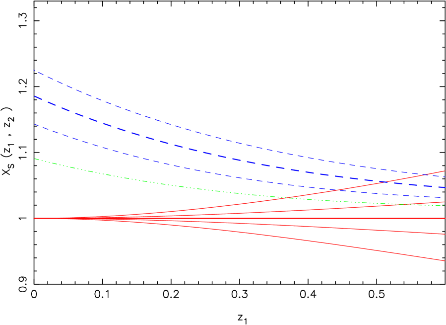
Figure 2: This figure shows both sides of inequality 14 as a function of redshift $z_{1}$. The solid lines show the right-hand side of 14, i.e. the upper limit on $X_{S}$ for non-accelerated models, assuming respective curvature radii $R_{C}=-0.6$, $-1.0$, $\infty$, $+1.0$, $+0.6$ in units of $c/H_{0}$ (bottom to top). The dashed lines show the predicted values of $X_{S}(z_{1},z_{2})$ for varying $z_{1}$ at fixed $z_{2}=z_{acc}$, for the same four models as in Fig. 1. The three dashed lines show flat $\Lambda$CDM models with $\Omega_{m}=0.24$ (upper), 0.27 (thick), 0.31 (lower). The dot-dashed line shows wCDM with $\Omega_{m}=0.32$, $w=-0.85$.

In the above Eq. 14, the square bracket term in $X_{S}$ is given to first order by $(1+\frac{2}{3}z_{1})^{-1}$. Higher order terms are small, and a quadratic approximation is not an improvement; a slightly better approximation is $(1+0.65\,z_{1})^{-1}$ which is accurate to $0.2\%$ for $z_{1}\leq 0.3$. Note that the RHS of (14) has no dependence on $z_{2}$; the curvature radius $R_{C}$ has no effect on the observable $y(z_{2})$ since $y$ is purely a line-of-sight measurement. Therefore, we may choose to measure $y(z_{2})$ anywhere, but if the real universe is accelerating, the observed $X_{S}$ will be maximal when $z_{2}$ is close to the past minimum of $y(z_{2})$, at $z_{2}\approx z_{\rm acc}$.

3.3 Predictions for $\Lambda$CDM

In Figure 2 we show predictions for $X_{S}(z_{1},z_{2})$ as a function of $z_{1}$ for three $\Lambda$CDM models (dashed) and one wCDM model (dash-dot), from substituting Eq. 12 into 14 and evaluating $H(z)$ and $D_{V}(z)$ for the models. For each of these plotted curves, $z_{2}$ is set to $z_{\rm acc}$ for that model. The non-accelerating upper limit for $X_{S}$ (the RHS of Eq. 14) is shown as solid lines for several assumed values of curvature radius $R_{C}$.

We see from Figure 2 that if the real universe has followed an expansion history $H(z)$ similar to $\Lambda$CDM prediction, inequality 14 will be violated if $z_{1}$ is reasonably small and $z_{2}$ is near $z_{acc}\sim 0.75$. Essentially, the accelerated expansion between $z_{2}$ and $z_{1}$ causes the value of $H(z)/(1+z)$ to be larger at $z\leq z_{1}$ than in the past at $z_{2}$, as in Figure 1; this makes $D_{V}(z_{1})$ smaller and $d(z)$ larger, compared to any non-accelerating model with the same $H(z_{2})$, so $X_{S}$ violates the limit in Eq. 14.

As noted above, to maximise the violation we should choose $z_{2}$ to minimise the observed value of $y(z_{2})$, i.e. the redshift $z_{\rm acc}$ where $H(z)/(1+z)$ had its past minimum; for a $\Lambda$CDM model with $\Omega_{m}=0.27$, the actual minimum is at $z_{\rm acc}\approx 0.75$, but the theoretical $y(z)$ is within 2% of its minimum value over a rather broad window $0.5\mathrel{\lower 2.58334pt\hbox{$\buildrel{\textstyle<}\over{\scriptstyle\sim}$}}z\leq 1.1$: so for an observational application of the test, $z_{2}$ may be whatever is most convenient observationally within this range, with only marginal weakening of the trap.

Turning to the variation of $X_{S}$ with $z_{1}$, the predicted value of $X_{S}$ is maximal at $z_{1}=0$ (with a value of 1.185 for our reference model C), and slowly declines with $z_{1}$: thus lower $z_{1}$ is better both to maximise lever-arm in our speed-trap, and to minimise curvature uncertainty. However, for practical observations $z_{1}$ cannot be too small since we need sufficient cosmic volume to get a robust detection of the acoustic feature in the galaxy correlation function $\xi(r)$ or power spectrum $P(k)$; therefore there is a tradeoff between $X_{S}$ which declines with $z_{1}$, the curvature uncertainty also favours smaller $z_{1}$, but the available cosmic volume for measuring $d(z_{1})$ grows with $z_{1}$. Thus for an observational application of the speed-trap, there is an optimal window around $0.15\mathrel{\lower 2.58334pt\hbox{$\buildrel{\textstyle<}\over{\scriptstyle\sim}$}}z_{1}\mathrel{\lower 2.58334pt\hbox{$\buildrel{\textstyle<}\over{\scriptstyle\sim}$}}0.35$.

Taking example values $z_{1}=0.1$, $0.2$, $0.3$, the concordance model predicts $X_{S}(z_{1},\,0.75)=1.145$, $1.113$, $1.088$ respectively. We also note that the value of $X_{S}$ is fairly sensitive to the value of $\Omega_{m}$: taking example cases from Table 1 with $\Omega_{m}=0.24,0.27,0.31$ to bracket the plausible range, we find that $X_{S}(0,z_{\rm acc})=1.225$, 1.185, 1.143 respectively; while $X_{S}(0.2,z_{\rm acc})$ is 1.142, 1.113, 1.081. For each model, $X_{S}-1$ approximately halves from $z_{1}=0$ to $z_{1}\approx 0.27$. This is because the rate of acceleration grows with time after $z_{\rm acc}$, so $X_{S}$ has stronger than linear dependence on $q_{0}$.

We note here that the prediction for $X_{S}$ is independent of $H_{0}$ if all of $\Omega_{m}$, $\Omega_{DE}$, $\Omega_{k}$ and $w$ are held fixed. However, since our example models are approximately CMB-matched, a correlation appears, because raising $\Omega_{m}$ and/or $w$ compared to the concordance model requires lowering $H_{0}$ to remain consistent with the CMB; while raising $\Omega_{m}$ or $w$ also leads to weaker acceleration and thus lowers $X_{S}$. Thus, $X_{S}$ at a fixed redshift is positively correlated with $H_{0}$ in CMB-matched Friedmann models.

We also note that for accelerating models $X_{S}$ remains a few percent greater than 1 for the case $z_{1}=z_{2}$; this occurs because $y(z_{2})$ measures the instantaneous expansion rate at $z_{2}$, while $d(z_{1})$ depends on the average expansion rate at redshifts below $z_{1}$, which is larger. In principle we could use this to test acceleration by measuring $d$ and $y$ from a single survey at $z_{1}=z_{2}$, but in practice the curvature uncertainty probably disfavours this (see Sec 4.5 for more discussion).

4 Discussion

In this section we discuss various aspects of the test above, including possible shifts in length $r_{s}$, useful approximations for $D_{V}(z)$, observational issues, the relation to the Alcock-Paczynski ratio and the effect of giant-void models.

4.1 Possible shifts in $r_{s}$

In applying the speed-trap, clearly assumptions (i) and (ii) above are very basic; if future observations show the speed-trap is observationally violated, we need to be confident that assumption (iii) on constancy of $r_{s}$ is valid to around $\sim 2\%$, in order to reject general homogeneous non-accelerating models with high confidence.

We now consider some details which may actually give rise to a significant shift in comoving $r_{s}$ between redshifts $z_{1}$ and $z_{2}$; the main such effects are galaxy bias, non-linear growth of structure, redshift-space distortions (Kaiser, 1987; Hamilton, 1992), and possible effects due to the hump(s) sitting on a sloping background power spectrum etc.

We first note that there is non-negligible evolution in $r_{S}$ at high redshift between $z_{d}\approx 1020$ and $z\sim 10$, as shown by Figure 1 of Eisenstein, Seo & White 2007; the initial BAO bump is only in the baryons and photons, and the peak shifts slightly as the dark-matter and baryon perturbations align together at later times; this implies the late-time BAO peak is not exactly at the sound horizon length $r_{S}(z_{d})$. However, after $z\mathrel{\lower 2.58334pt\hbox{$\buildrel{\textstyle<}\over{\scriptstyle\sim}$}}10$ the density perturbations in baryons and dark matter are very similar. In most real BAO analyses, a matter power spectrum from CMBFast or similar is used, together with a model for non-linear evolution and an arbitrary linear “stretch factor” $\alpha$, to fit observations; finally, the measurement is quoted as $d(z)=\alpha\,r_{S}(z_{d})/D_{V}(z)$ where $r_{S}$ and $D_{V}$ are both computed from the reference theoretical model. This implies that small errors in the reference model should (on average) be absorbed into an opposite shift in $\alpha$, so the final estimate of $d(z)$ should be unbiased. Any shift in the BAO length from $z\sim z_{d}$ to $z\sim 10$ is included in the reference model; therefore, $r_{S}(z_{d})$ forms essentially a convenient fiducial length for intercomparison between models, which is close to but not exactly the position of the low-redshift BAO peak in the correlation function. For the present work, we are only interested in shifts of the BAO scale at $z<z_{2}\sim 0.75$, so the above effect cancels.

Galaxy bias, at least in standard versions, has little effect since the BAO scale is very much larger than any scale of relevance for galaxy formation; thus bias may affect the overall amplitude of galaxy clustering but cannot significantly shift the scale $r_{s}$. Likewise, non-linear growth of structure primarily moves galaxies around on $\sim 5\,h^{-1}\,{\rm Mpc}$ scales; this significantly blurs the bump in $\xi(r)$, and/or erases the higher harmonics in the power spectrum, but this is almost symmetrical between inward and outward shifts: the systematic shift in the BAO lengthscale is much smaller.

For the standard model, these effects have been investigated from both theory by e.g. Eisenstein, Seo & White (2007) and Shoji, Jeong & Komatsu (2009), and from large N-body simulations by Seo et al (2008) and Seo et al (2010); these papers agree that systematic shifts are small, typically below the $0.6\%$ level at $z=0.3$ and less at higher redshift. They also find that reconstruction methods based on velocity-field reconstruction (Eisenstein et al, 2007) can reduce the shift to $\sim\,0.1\%$. This will become important for the next generation of ambitious planned surveys such as ESA’s Euclid (e.g. Samushia et al 2011) or NASA’s WFIRST, which aim to achieve sub-percent precision on BAO observables in many redshift bins, but are almost negligible with respect to the speed-trap test in this paper.

We caution that there is a slight level of circular argument in the above, in that we are assuming standard cosmology to limit the shift in $r_{s}$, and then using this to reject non-standard non-accelerating models; it remains possible that a model with non-standard gravity could produce a much larger shift in $r_{s}$ than the standard cosmology. However, non-standard models producing a gross $\sim 10\%$ shift in $r_{s}$ since $z_{2}\sim 0.75$ would almost certainly produce large levels of redshift-space distortion, and give strong inconsistencies between the angular and radial measurements of $r_{s}$ at low redshift. If both the redshift-space distortion pattern and the radial and angular measurements of $r_{s}$ are measured to be consistent with standard $\Lambda$CDM, this would strongly suggest that the true shifts in $r_{s}$ should not be much larger than the percent level effects predicted by the standard model.

4.2 Approximations for $D_{V}$

As an aside, we also note that in nearly-flat CDM-like models, an accurate approximation to $D_{V}(z)$ at moderate redshift is given by Taylor-expanding $1/H(z)$ around $z/2$ (rather than zero), and substituting in the integral Eq. 4; this makes $z^{2}$ terms vanish, and leads to the approximation

$$D_{V}(z)\approx{cz\over[H^{2}(z/2)\,H(z)]^{1/3}}+O(z^{3})\ ;$$ (15)

in practice the first term is surprisingly accurate for $\Lambda$CDM models, with errors $<0.1\%$ compared to the numerical result for $z<0.5$. (See Appendix A for evaluation of the third-order term, and explanation why it is small).

A simpler approximation is

$$D_{V}(z)\approx{cz\over H(2z/3)}\ ;$$ (16)

this is slightly less accurate than the previous approximation, but still accurate to $<0.4\%$ for $z<0.5$, better than the mid-term precision on observables. (For open zero-$\Lambda$ models these approximations are less good, with errors up to $2\%$).

While it is straightforward to evaluate $D_{V}$ and $X_{S}$ numerically for any given model, the main value of this approximation is that it tells us that a measurement of $z\,d(z)$ at low redshift is quite close to a measurement of $r_{s}H(2z/3)/c$ ; substituting this into (14), along with the approximation $(1+\frac{2}{3}z_{1})^{-1}$ for the square-bracket term, gives simply

$$X_{S}(z_{1},z_{2})\approx{(1+z_{2})\over H(z_{2})}{H\left(\frac{2}{3}z_{1}\right)\over 1+\frac{2}{3}z_{1}}={\dot{a}(\frac{2}{3}z_{1})\over\dot{a}(z_{2})}\ ;$$ (17)

and inequality 3 tells us this should be less than 1 for non-accelerated models. Unlike our upper limit Eq. (14) this expression is not rigorous, but this gives a simple and fairly accurate approximation for what $X_{S}$ is measuring, i.e. it is closely related to the ratio of expansion rates $\dot{a}$ at $\frac{2}{3}z_{1}$ compared to $z_{2}$.

4.3 Observational advantages

One possible objection to this test is that it is comparing two related but slightly different observables, i.e. a spherical-average scale at $z_{1}$ with a radial scale at $z_{2}$. Why have we done this, rather than comparing two measures of $d(z)$ or two measures of $y(z)$ at two different redshifts ?

It is well known that comparing $y(z)$ at two different redshifts provides another direct test of acceleration. The main difficulty is observational, since for our baseline model, $y(z_{1})$ only grows to $1.1\,y(z_{acc})$ at rather low redshift $z_{1}\sim 0.16$. Furthermore, for a given survey, a radial-only measurement of $r_{s}$ has a statistical error roughly $\sqrt{3}$ worse than a spherical average measure. Even if we had a $3\pi$ steradian redshift survey at $z_{1}\approx 0.16$, we may not do much better than 3% statistical error on $y$, a $3\sigma$ violation, and we would like to get above $5\sigma$ for a decisive result. Using $d(z_{1})$ instead of $y$ gives two substantial advantages: firstly $d(z_{1})$ effectively measures $H$ at $\sim 2z_{1}/3$, giving more lever-arm on the low-redshift acceleration; so a measurement of $d(z_{1}=0.24)$ is similar in content to a measurement of $y(z_{1}=0.16)$. Secondly there is the obvious gain that $d$ uses 3 spatial directions instead of 1. Thus for a fixed thickness of survey shell, the former measure has around 9/4 times more available volume and 3 independent axes, so the cosmic variance limit should improve by a factor $\sim\sqrt{27/4}\approx 2.6$, which is a very important practical advantage.

In contrast, comparing $d(z)$ at two different redshifts suffers from potential major uncertainty in cosmic curvature at the high redshift $z_{2}$. At $z_{2}\approx 0.75$ there is ample available volume for a precision measurement of $y$, and ambitious future probes such as Euclid (Samushia et al 2011) plan to push to statistical errors $\mathrel{\lower 2.58334pt\hbox{$\buildrel{\textstyle<}\over{\scriptstyle\sim}$}}0.75\%$ on both $y$ and $d$, in each of many bins of width 0.1 in redshift. Thus, at $z_{2}$ the cosmic variance is minimal for a wide-area survey, so the radial measure is preferable because it is independent of the curvature nuisance parameter. Also, $d(z_{2})$ depends on the full history of $H(z)$ back to $z_{2}$, which complicates the issue of deriving an inequality.

In our proposed comparison, we have constructed a ratio $X_{S}$ using $d(z_{1})$ at low redshift and $y(z_{2})$ at the higher redshift, to circumvent both of these problems: the potential cosmic-variance limits are probably around $1\%$ on $d(0.24)$ and significantly less on $y(0.75)$, so this test can (given ample data) deliver a standalone rejection of homogeneous non-accelerating models at $\sim 7\sigma$ significance level. This can be further improved by using several independent redshift bins, e.g. $z_{1}=0.15,0.25$ and $z_{2}=0.65,0.75$.

4.4 Future Observations

As noted above, there already exist measurements of the numerator on the left of Eq. 13 from Percival et al (2010); they quote values of $d(0.2)=0.1905$ and $d(0.35)=0.1097$, with approximately 3.3% error on each. For the numerator $z\,d(z)$ in inequality (14) these give $0.2\,d(0.2)=0.0381$ and $0.35\,d(0.35)=0.0384$.

As yet there is no available measurement of radial BAOs at $z>0.5$ with which to actually calibrate our speed-trap, but these are expected soon from the recently completed AAT WiggleZ survey (Blake et al, 2010), and in a few years from the ongoing BOSS survey (White et al, 2011). It is currently unclear whether the final WiggleZ survey covers enough volume to separately measure the radial component as required here, but BOSS should very likely achieve this; the upper redshift limit of BOSS is $\approx 0.65$, so this is close enough to $z_{\rm acc}$ to be useful.

For $\Lambda$CDM, the predicted value of $y(z_{2})$ near its minimum is approximately 0.0302 for $\Omega_{m}=0.27$ and $H_{0}=70\,{\rm km\,s^{-1}\,Mpc^{-1}}$. For reasonable variations of parameters, we now show that if we assume a flat universe then $y(z_{2})$ is well constrained by CMB observations: it is well known that for flat models with varying $\Omega_{m},h,w$ there is a tight correlation between the age of the Universe, $t_{0}$, and the CMB acoustic scale $\ell_{A}$ (Knox et al, 2001); and it turns out that there is also a tight correlation between these and the value of $H$ at intermediate redshift, with a pivot point occurring at $z\approx 0.8$ (see Figure 1). This is partly a coincidence, because for moderate parameter variations around the concordance model, $t_{0}$ scales $\propto\Omega_{m}^{-0.3}h^{-1}$, while $\ell_{A}$ scales as $\Omega_{m}^{-0.15}h^{-0.5}$. For the value of $H(z)$, we note that as $z\rightarrow 0$ this scales as $h$ independent of $\Omega_{m},w$, while at $z\mathrel{\lower 2.58334pt\hbox{$\buildrel{\textstyle>}\over{\scriptstyle\sim}$}}3$ where dark energy is negligible, $H(z)$ scales $\propto\Omega_{m}^{0.5}h^{1}$. Therefore, there exists a pivot-point at intermediate redshift where $H(z)$ scales as $\Omega_{m}^{0.3}h$ (i.e. inversely to $t_{0}$), and this pivot redshift turns out to be $z\approx 0.85$ for $\Lambda$ models. For $w>-1$ the pivot redshift is somewhat lower, but for near-flat Friedmann models the value $H(z=0.75)$ is better constrained by WMAP data than the local $H_{0}$; and fixing $t_{0}\approx 13.75\,{\rm Gyr}$ constrains $H(z=0.75)/(1.75)=59.2\,{\rm km\,s^{-1}\,Mpc^{-1}}$ within $\approx 0.8\%$, which in turn leads to a tight prediction for $y(0.75)$.

(As an aside, there is a corollary that if some future method could give a direct measurement of $H(z=0.75)$ independently of $r_{S}$, this would produce another strong consistency test of standard $\Lambda$CDM. This may be possible in principle using methods such as differential-age measurements of early-type galaxies, or lensing measurements with source and lens close in redshift, but this will require a major advance in precision over current data).

Assuming some future $y$ measurement turns out at the concordance value $y(z_{2})\approx 0.0302$, we would then obtain measurements $X_{S}\approx 1.12$ and 1.05 at $z_{1}=0.2$, 0.35 respectively. The error on $y(z_{2})$ must be added in quadrature to the current 3.3% error on $d(z_{1})$, but if the former is around 2% then we can anticipate a fairly clear violation from the $z=0.2$ value, and a somewhat less significant violation at $z=0.35$.

The prospects are good for improving on the current results: the projections for the BOSS survey (White et al, 2011) are for $1\%$ precision on $d(z=0.35)$, and precision of $1.7\%$ on $y(0.6)$. Adding the above errors in quadrature leads to around 2% precision on $X_{S}$, with a predicted value $\approx 1.077$, thus nearly a $4\sigma$ proof of acceleration. BOSS may also do better using the larger value of $X_{S}$ at $z_{1}\sim 0.2$, but projected precision on $d(0.2)$ is not quoted separately.

Next-generation surveys in the planning stage such as BigBOSS, Euclid or WFIRST should substantially improve on the higher-redshift measurement, reaching sub-percent precision on $y(z_{2})$. The low-redshift $d(z_{1})$ measurement is ultimately limited by cosmic variance, but extending the BOSS survey to the Southern hemisphere can give a straightforward improvement by a factor of $\sqrt{2}$, or probably more if denser sampling of galaxies is used. Further improvements are possible in principle using HI or near-infrared selected surveys which can cover $>80\%$ of the whole sky, compared to $\sim 50\%$ for visible-selected surveys.

4.5 Comparison with the Alcock-Paczynski test

We note here that our ratio $X_{S}$ may be considered as a generalised version of the classic test of Alcock & Paczynski (1979), hereafter AP: the AP ratio was defined to be $R_{AP}\equiv\Delta z/z\Delta\theta$, which in our notation becomes

$$R_{AP}(z)\equiv{(1+z)D_{A}(z)H(z)\over cz}\ .$$ (18)

If we choose $z_{1}=z_{2}$ in Eq. 12 above and substitute Eq. 1 for $D_{V}$, we then obtain

$${z_{1}d(z_{1})\over y(z_{1})}=(1+z_{1})R_{AP}(z_{1})^{-2/3}$$ (19)

thus $X_{S}(z_{1},z_{1})$ contains the same information as $R_{AP}(z_{1})$ combined with a function of $z_{1}$; substituting the above into Eq. 14 gives a lower limit on $R_{AP}$ for non-accelerating models, which is

$$R_{AP}(z_{1})\geq{(1+z_{1})\ln(1+z_{1})\over z_{1}}{S_{k}(x_{1})\over x_{1}}\ .$$ (20)

It is well known that if we assume the Friedmann equations, the AP test at high redshift provides a strong test for $\Lambda$ or dark energy: however, if we drop the Friedmann connection between curvature and matter content, then at $z\mathrel{\lower 2.58334pt\hbox{$\buildrel{\textstyle>}\over{\scriptstyle\sim}$}}0.5$ the AP test becomes mostly degenerate between acceleration and curvature. At lower $z<0.4$, we may use the approximation $(1+z)D_{A}(z)\approx cz/H(z/2)$ from above, which leads to $R_{AP}(z_{1})\approx H(z_{1})/H(\frac{z_{1}}{2})$. This does have more sensitivity to acceleration than curvature, but is not ideal for the following reason: at small $z_{1}$ the AP ratio suffers from a short redshift lever-arm, while at $z_{1}\mathrel{\lower 2.58334pt\hbox{$\buildrel{\textstyle>}\over{\scriptstyle\sim}$}}0.4$ the ratio mainly probes the regime of sluggish acceleration at $z>0.2$. The AP ratio at $z_{1}\approx 0.4$ may provide a useful test, but will probably require sub-percent level precision on both observables to get a decisive result.

Compared to the AP test, the use of two widely-spaced redshifts in $X_{S}$ requires the added assumption that $r_{S}$ has minimal evolution between $z_{2}$ and $z_{1}$, but enables a much longer effective time lever-arm, giving a larger acceleration signal while keeping the curvature sensitivity very small.

4.6 Inhomogeneous Void Models

Recently there has been some interest in models which produce apparent acceleration without dark energy, by placing us near the centre of a giant underdense spherical void, with a Lemaitre-Tolman-Bondi metric; examples are in Tomita (2009) and references therein. These models have several problems such as severe fine-tuning of our location very close to the void centre, and probable inconsistency with limits on the kinetic Sunyaev-Zeldovich effect (Zhang & Stebbins, 2011); however it is interesting to note how $X_{S}$ behaves in such models. A recent confrontation of giant-void models with BAO observables has been done by Moss, Zibin & Scott (2011): they find that void models with profiles adjusted to match SNe and CMB observations have a $\Delta z_{/\!/}$ which is $\mathrel{\lower 2.58334pt\hbox{$\buildrel{\textstyle>}\over{\scriptstyle\sim}$}}30\%$ smaller at $z\sim 0.5-0.7$ compared to $\Lambda$CDM. Those specific cases would have $X_{S}(0.2,0.75)\mathrel{\lower 2.58334pt\hbox{$\buildrel{\textstyle>}\over{\scriptstyle\sim}$}}1.4$, which is substantially larger than any reasonable dark-energy model; thus, Moss, Zibin & Scott (2011) show that giant-void models matched to angular distances and the CMB appear to suffer from severe “overkill” in radial BAO measurements.

The parameter space of possible void models is very large, so other void models may look more similar to $\Lambda$CDM, but we note that the test of Clarkson, Bassett & Lu (2008) can be used to test for homogeneity without assuming GR. They show that if we have both angular and radial BAO measurements spanning a range of redshift, there is a consistency relation which must be satisfied by homogeneous models but is usually violated by giant-void models. Thus, assumption (i) above becomes observationally testable using future BAO observations, though this probably requires observations spanning more redshifts than the $X_{S}$ test here.

5 Conclusions

We have proposed a new and simple smoking-gun test for cosmic acceleration using only a comparison of the baryon acoustic oscillation feature at two distinct redshifts $\sim 0.2$ and $\sim 0.75$. The main result of our paper is inequality (14) relating the two dimensionless BAO observables, which must be satisfied for any homogeneous non-accelerating model, but will be observationally violated by $\approx 10\%$ in models with an expansion history close to standard $\Lambda$CDM.

Clearly, our proposed measurement has advantages and disadvantages: the main advantages are extreme simplicity and model-independence, i.e. if the inequality (14) is violated, we can rule out essentially all homogeneous non-accelerating models in one shot, without assuming any particular gravity theory or parametric form of $H(z)$, and independent of supernova and CMB observations.

The main drawback of our test is that it is essentially one-sided: if inequality 14 is observationally violated, we have proved (given some basic assumptions) that acceleration has occurred during $0\leq z\leq z_{2}$ and have a rough quantification of the amount, but no more details about the underlying cause or the details of the expansion history.

If we assume GR and the Friedmann equations hold, and that $r_{s}$ has the value which is accurately predicted from CMB analysis, then we have much more statistical power: future measurements of BAOs in many redshift bins may be used to reconstruct the detailed form of the expansion history $H(z)$; this can be integrated to give predictions of $D_{R}(z)$, and comparison with the measured transverse BAO scale giving $D_{A}(z)$ can constrain spatial curvature independent of the CMB; while comparison of $D_{A}$ with $D_{L}(z)$ from SNe can check the distance-duality or Tolman relation $(D_{L}/D_{A})^{2}=(1+z)^{4}$. All of this can give much more powerful cross-checks and parameter estimates than our simplified one-sided test.

However, our proposed cosmic speed-trap seems to provide a valuable addition to the set of cosmological measurements, due to its bare minimum of assumptions. This provides a strong motivation for future improved BAO measurements specifically near redshifts $\sim 0.25$ and 0.75; this should preferably include a low-redshift survey comparable or superior to BOSS in the Southern hemisphere to minimise the cosmic variance in the local measurement.

Appendix A The approximation for $D_{V}$

We here add a note which explains the surprisingly good accuracy of approximation 15 for $D_{V}(z)$ at fairly low redshift $z<0.4$. As noted, in the integral Eq. 4 for $D_{R}$, it is helpful to Taylor-expand the function $1/H(z)$ around the mid-point of the integral at $z_{1}/2$, then integrate: this naturally makes terms with odd-integer derivatives of $1/H$ integrate to zero, and leads to

$$D_{R}(z_{1})\approx c\left[{z_{1}\over H(\frac{z_{1}}{2})}+{z_{1}^{3}\over 24}\left({1\over H}\right)^{\prime\prime}(\frac{z_{1}}{2})+O(z_{1}^{5})\right]$$ (21)

where prime denotes $d/dz$. We now need the second derivative $(1/H)^{\prime\prime}$ evaluated at $\frac{z_{1}}{2}$. Defining the usual deceleration parameter $q$ and the jerk parameter $j$ (e.g. Alam et al 2003) as

$$q\equiv-{d^{2}a/dt^{2}\over aH^{2}}\ ,\qquad j\equiv{d^{3}a/dt^{3}\over aH^{3}}\ ,$$ (22)

we can rearrange these in terms of $d/dz$ to get

$${dH\over dz}={H\over 1+z}(1+q)\ ,\qquad{d^{2}H\over dz^{2}}={H\over(1+z)^{2}}(j-q^{2})\ .$$ (23)

Using these we obtain

$${d^{2}\over dz^{2}}\left(\frac{1}{H}\right)={-j+2+4q+3q^{2}\over(1+z)^{2}\,H}\ .$$ (24)

For the case of flat $\Lambda$CDM models, $j=+1$ independent of parameters (assuming radiation density is negligible) (Rapetti et al, 2007), thus the numerator in Eq. 24 has zeros at $q=-1/3$ and $q=-1$. For $\Omega_{m}$ near the concordance model, $q$ passed through $-1/3$ in the fairly recent past at $z\sim 0.3$, so the numerator is significantly smaller than unity at low redshift. This explains qualitatively the very good accuracy of approximation 15 near the concordance model, even up to significant redshifts $z\approx 0.5$.

References

- Abdalla et al (2010) Abdalla F.B., Blake C., Rawlings S., 2010, MNRAS, 401, 743.
- Alam et al (2003) Alam U., Sahni V., Saini T-D., Starobinsky A.A., 2003, MNRAS, 344, 1057.
- Alcock & Paczynski (1979) Alcock C. & Paczynski B., 1979, Nature, 281, 358.
- Allen et al (2011) Allen S., Evrard A., Mantz A., 2011, ARAA, 49, 409.
- Bassett & Hlozek (2010) Bassett B.A. & Hlozek R., 2010, in “Dark Energy”, ed P. Ruiz-Lapuente, Cambridge Univ. Press.
- Blake & Glazebrook (2003) Blake C. & Glazebrook K., 2003, ApJ, 594, 665.
- Beutler et al (2011) Beutler F., Blake C., Colless M. et al, 2011, MNRAS, 416, 3017.
- Blake et al (2010) Blake C., Brough S., Colless M. et al, 2010, MNRAS, 406, 803.
- Blake et al (2011) Blake C., Davis T., Poole G. et al, 2011, MNRAS, 415, 2892
- Carnero et al (2012) Carnero A., Sanchez E., Crocce M., Cabre A., Gaztanaga E., 2012, MNRAS, 419, 1689.
- Clarkson, Bassett & Lu (2008) Clarkson C., Bassett B., Lu T., 2008, PRL, 101.011301
- Cole et al (2005) Cole S., Percival W.J., Peacock J.A. et al, 2005, MNRAS, 362, 505.
- Conley et al (2011) Conley A. et al, 2011, ApJS, 192, 1.
- Eistenstein & Hu (1998) Eisenstein D.J. & Hu W., 1998, ApJ, 496, 605.
- Eisenstein et al (2005) Eisenstein D.J., Zehavi I., Hogg D. et al, 2005, ApJ, 633, 560.
- Eisenstein et al (2007) Eisenstein D.J, Seo H., Sirko E., Spergel D.N., 2007, ApJ, 664, 675.
- Eisenstein, Seo & White (2007) Eisenstein D.J, Seo H., White M., 2007, ApJ, 664, 660.
- Frieman, Turner & Huterer (2008) Frieman J., Turner M., Huterer D., 2008, ARAA, 46, 385.
- Gaztanaga et al (2009) Gaztanaga E., Cabre A., Hui L., 2009, MNRAS, 399, 1663.
- Guy et al (2010) Guy J., Sullivan M., Conley A. et al 2010, A&A, 523, 7.
- Hamilton (1992) Hamilton A.J.S., 1992, ApJ, 385, L5.
- Kaiser (1987) Kaiser N., 1987, MNRAS, 227, 1.
- Kazin et al (2010) Kazin E.A., Blanton M.R., Scoccimarro R. et al, 2010, ApJ, 710, 1444.
- Knox et al (2001) Knox L., Christensen N., Skordis C., 2001, ApJ, 563, 95.
- Komatsu et al (2011) Komatsu E., Smith K., Dunkley J. et al, 2011, ApJS, 192, 18.
- Larson et al (2010) Larson D., Dunkley J., Hinshaw G. et al, 2011, ApJS, 192, 16.
- Linder (2008) Linder E., 2008. Gen. Rel. Grav., 40, 329.
- Liske et al (2008) Liske J., Grazian A., Vanzella E. et al, 2008, MNRAS, 386, 1192.
- Meiksin, White & Peacock (1999) Meiksin A., White M. & Peacock J.A., 1999, MNRAS, 304, 851.
- Moss, Zibin & Scott (2011) Moss A., Zibin J.P. & Scott D., 2011, Phys.Rev.D, 83, 103515.
- Peacock (1999) Peacock J.A., 1999, “Cosmological Physics”, Cambridge Univ. Press.
- Peebles & Yu (1970) Peebles P.J.E. & Yu J.T, 1970, ApJ, 162, 815.
- Percival et al (2010) Percival W.J., Reid B., Eisenstein D.J. et al, 2010, MNRAS, 401, 2148.
- Rapetti et al (2007) Rapetti D., Allen S., Amin M., Blandford R., 2007, MNRAS, 375, 1510.
- Riess et al (2007) Riess A.G., Strolger L-G., Casertano S. et al, 2007, ApJ, 659, 98.
- Samushia et al (2011) Samushia L., Percival W.J., Guzzo L. et al, 2011, MNRAS, 410, 1993.
- Seo & Eisenstein (2003) Seo H-J., Eisenstein D.J., 2003, ApJ, 598, 720.
- Seo et al (2010) Seo H-J., Eckel J., Eisenstein D.J. et al, 2010, ApJ, 720, 1650.
- Seo et al (2008) Seo H-J., Siegel E.R., Eisenstein D.J., White M., 2008, ApJ, 636, 13.
- Shapiro & Turner (2006) Shapiro C. & Turner M.S., 2006, ApJ, 649, 563.
- Shoji, Jeong & Komatsu (2009) Shoji M., Jeong D., Komatsu E., 2009, ApJ, 693, 1404.
- Tian et al (2011) Tian H.J., Neyrinck M.C., Budavari T., Szalay A.S., 2011, ApJ, 728, 34.
- Tomita (2009) Tomita K., 2009, arXiv.org/0906.1325
- White et al (2011) White M., Blanton M., Bolton A. et al, 2011, ApJ, 728, 126.
- Zhang & Stebbins (2011) Zhang P. & Stebbins A., 2011, Phys. Rev. Lett, 107, 041301.