Protocols for Relay-Assisted Free-Space Optical Systems

Abstract

We investigate transmission protocols for relay-assisted free-space optical (FSO) systems, when multiple parallel relays are employed and there is no direct link between the source and the destination. As alternatives to all-active FSO relaying, where all the available relays transmit concurrently, we propose schemes that select only a single relay to participate in the communication between the source and the destination in each transmission slot. This selection is based on the channel state information (CSI) obtained either from all or from some of the FSO links. Thus, the need for synchronizing the relays’ transmissions is avoided and the slowly varying nature of the atmospheric channel is exploited. For both relay selection and all-active relaying, novel closed-form expressions for their outage performance are derived, assuming the versatile Gamma-Gamma channel model. Furthermore, based on the derived analytical results, the problem of allocating the optical power resources to the FSO links is addressed, and optimum and suboptimum solutions are proposed. Numerical results are provided for equal and non-equal length FSO links, which illustrate the outage behavior of the considered relaying protocols and demonstrate the significant performance gains offered by the proposed power allocation schemes.

I Introduction

The constant need for higher data rates in support of high-speed applications has led to the development of the Free Space Optical (FSO) communication technology. Operating at unlicensed optical frequencies, FSO systems offer the potential of broadband capacity at low cost [1], and therefore, they present an attractive remedy for the ”last-mile” problem. However, despite their major advantages, the widespread deployment of FSO systems is hampered by major impairments, which have their origin in the propagation of optical signals through the atmosphere. Rain, fog, and atmospheric turbulence are some of the major atmospheric phenomena that cause attenuation and rapid fluctuations in the received optical power in FSO systems, thereby increasing the error rate and severely degrading the overall performance [2].

In the past, several techniques have been applied in FSO systems for mitigating the degrading effects of the atmospheric channel, including error control coding in conjunction with interleaving [3], multiple-symbol detection [4], and spatial diversity [5, 6, 7]. Among these techniques, spatial diversity, which is realized by deploying multiple transmit and/or receive apertures, has been particularly attractive, since it offers significant performance gains by introducing additional degrees of freedom in the spatial dimension. Thus, numerous FSO systems with multiple co-located transmit and/or receive apertures, referred as Multiple-Input Multiple-Output (MIMO) FSO systems, have been proposed in the technical literature [5, 6, 7]. However, in practice, MIMO FSO systems may not always be able to offer the gains promised by theory. This happens in cases where the assumption that all the links of the MIMO FSO system are affected by independent channel fading becomes invalid [7]. Furthermore, since both the path loss and the fading statistics of the channel are distance-dependent, a large number of transmit and/or receive apertures is required in long-range links in order to achieve the desired performance gains, thus increasing the complexity of MIMO FSO systems.

In order to overcome such limitations, relay-assisted communication has been recently introduced in FSO systems as an alternative approach to achieve spatial diversity [8, 9, 10, 11]. The main idea lies in the fact that, by employing multiple relay nodes with line-of-sight (LOS) to both the source and the destination, a virtual multiple-aperture system is created, often referred as cooperative diversity system, even if there is no LOS between the source and the destination. In [8], various relaying configurations (cooperative diversity and multihop) have been investigated under the assumption of a lognormal channel model. Subsequently, several coding schemes for 3-way cooperative diversity FSO systems with a single relay and a direct link between the source and the destination have been proposed in [9], while the performance of such systems has been investigated in [10] and [11] assuming amplify-and-forward and decode-and-forward relaying strategies, respectively. It is emphasized that in all these previous works, all the available relays participated in the communication between the source and the destination, requiring perfect synchronization between the relays such that the FSO signals can arrive simultaneously at the destination, while the optical power resources are equally divided between all FSO links.

In view of the above, in this paper we present alternative transmission protocols which can be applied to relay-assisted FSO systems with no LOS between the source and the destination. For the signaling rates of interest, the atmospheric channel does not vary within one packet. Thus, channel state information (CSI) can be easily obtained for all or for some of the involved links. Capitalizing on this fact, the presented protocols select only a single relay to take part in the communication in every transmission slot, thus avoiding the need for synchronization between the relays. It should be noted that similar relay selection protocols have been also proposed in the context of radio-frequency relaying systems [12, 13, 14]. In particular, two types of relay selection protocols are presented: the select-max protocol that selects the relay that maximizes an appropriately defined metric and requires CSI from all the available FSO links, and the distributed switch and stay (DSSC) protocol which switches between two relays and requires CSI only from the FSO links used in the previous transmission slot. Furthermore, assuming the versatile Gamma-Gamma channel model [2] and decode-and-forward relay nodes, we derive novel closed-form analytical expressions for the outage performance of the proposed transmission schemes, as well as the scheme where all the available relays transmit simultaneously; thus, extending the analysis presented in [8] to the case of the Gamma-Gamma channel model. Finally, based on the derived outage results, we address the problem of optimizing the allocation of the optical power resources to the FSO links for minimization of the probability of outage; hence, rendering the relay-assisted FSO system under consideration more power efficient.

The remainder of the paper is organized as follows. In Section II, the system model and the considered relaying protocols are discussed. The outage performance of the relaying protocols under investigation is analyzed in Section III, while the problem of optimizing the allocation of the optical power resources to the FSO links is addressed in Section IV. Numerical results for various relay-assisted FSO architectures are presented in Section V, and, finally, concluding remarks are provided in Section VI.

II System Model

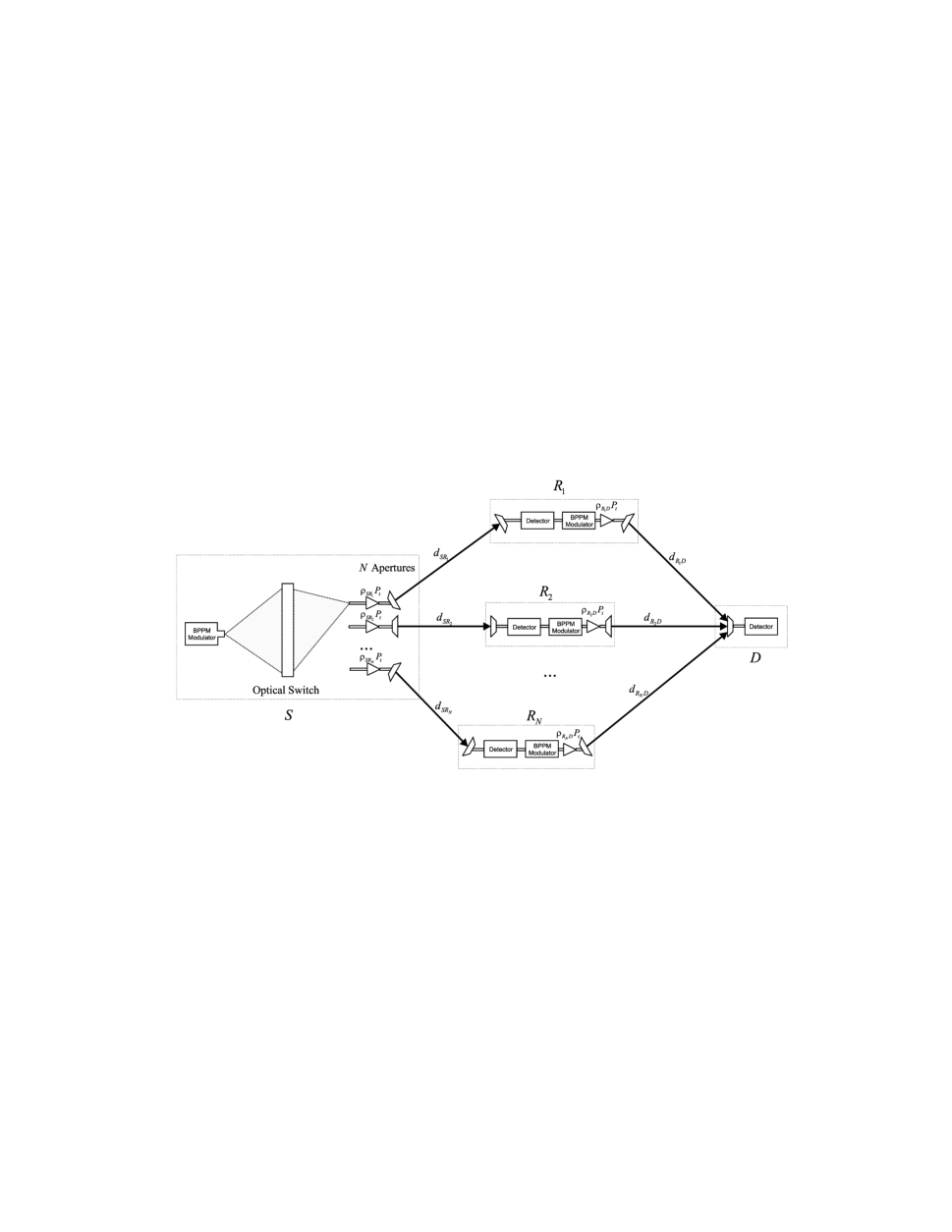
Figure 1: The relay-assisted FSO system under consideration.

The system model under consideration is depicted in Fig. 1. In particular, we consider an intensity-modulation direct detection (IM/DD) FSO system without LOS between the source, $S$, and the destination, $D$, and the communication between these two terminals is achieved with the aid of multiple relays, denoted by $R_{i}$, $i\in\left\{1,...,N\right\}$. The source node is equipped with a multiple-aperture transmitter, with each of the apertures pointing in the direction of the corresponding relay, and an optical switch, which either allows the simultaneous transmission from all the transmit apertures or selects the direction of transmission by switching between the transmit apertures.

The presence of a large field-of-view (FOV) detector at the destination is assumed allowing for the simultaneous detection of the optical signals transmitted from each relay. Moreover, all optical transmitters are equipped with optical amplifiers that adjust the optical power transmitted in each link. The relaying terminals use a threshold-based decode-and-forward (DF) protocol; that is, they fully decode the received signal and retransmit it to the destination only if the signal-to-noise ratio (SNR) of the receiving FSO link exceeds a given decoding threshold. Finally, throughout this paper, we assume that binary pulse position modulation (BPPM) is employed.

II-A Signal and Channel Model

For an FSO link connecting two terminals $A$ and $B$, the received optical signal at the photodetector of $B$ is given by

$$\mathbf{r}_{B}=\left[\begin{array}[]{c}r^{s}\\ r^{n}\end{array}\right]=\left[\begin{array}[]{c}\eta T_{b}\left(\rho_{AB}P_{t}h_{{}_{AB}}+P_{b}\right)+n^{s}\\ \eta T_{b}P_{b}+n^{n}\end{array}\right]$$ (1)

where $r^{s}$ and $r^{n}$ represent the signal and the non-signal slots of the BPPM symbol, respectively, while $\rho_{AB}P_{t}$ and $P_{b}$ denote the average optical signal power transmitted from $A$ and the background radiation incident on the photodetector of $B$, respectively. Furthermore, $\rho_{AB}$ represents the percentage of the total optical power $P_{t}$ allocated to the FSO link between terminals $A$ and $B$, $h_{{}_{AB}}$ is the channel gain of the link, $\eta$ is the photodetector’s responsivity, $T_{b}$ is the duration of the signal and non-signal slots, and $n^{s}$ and $n^{n}$ are the additive noise samples in the signal and non-signal slots, respectively. Since background-noise limited receivers are assumed, where background noise is dominant compared to other noise components (such as thermal, signal dependent, and dark noise) [5, 17], the noise terms can be modeled as additive white Gaussian, with zero mean and variance $\sigma_{n}^{2}=\frac{N_{0}}{2}$. After removing the constant bias $\eta T_{b}P_{b}$ from both slots, the instantaneous SNR of the link can be defined as [8]

$$\gamma_{{}_{AB}}=\frac{\eta^{2}\rho_{AB}^{2}T_{b}^{2}P_{t}^{2}h_{{}_{AB}}^{2}}{N_{0}}.$$ (2)

Due to atmospheric effects, the channel gain of the FSO link under consideration can be modeled as

$$h_{{}_{AB}}=\bar{h}_{{}_{AB}}\tilde{h}_{{}_{AB}}$$ (3)

where $\bar{h}_{AB}$ accounts for path loss due to weather effects and geometric spread loss and $\tilde{h}_{{}_{AB}}$ represents irradiance fluctuations caused by atmospheric turbulence. Both $\bar{h}_{{}_{AB}}$ and $\tilde{h}_{{}_{AB}}$ are time-variant, yet at very different time scales. The path loss coefficient varies on the order of hours while turbulence induced fading varies on the order of 1–100 ms [5]. Thus, taking into consideration the signaling rates of interest, which range from hundreds to thousands of Mbps, the channel gain can be considered as constant over a given transmission slot, which consists of hundreds of thousands (or even millions) of consecutive symbols.

The path loss coefficient can be calculated by combining the Beer Lambert’s law [2] with the geometric loss formula [1, pp. 44], yielding

$$\bar{h}_{{}_{AB}}=\frac{D_{R}^{2}}{\left(D_{T}+\theta_{T}d_{{}_{AB}}\right)^{2}}\exp\left(-vd_{{}_{AB}}\right)$$ (4)

where $D_{R}$ and $D_{T}$ are the receiver and transmitter aperture diameters, respectively; $\theta_{T}$ is the optical beam’s divergence angle (in $m$rad), $d_{{}_{AB}}$ is the link’s distance (in km), and $v$ is the weather dependent attenuation coefficient (in 1/km).

Under a wide range of atmospheric conditions, turbulence induced fading can be statistically characterized by the well-known Gamma-Gamma distribution [2]. The probability density function (pdf) for this model is given by

$$f_{\tilde{h}_{{}_{AB}}}\left(x\right)=\frac{2\left(\alpha_{{}_{AB}}\beta_{{}_{AB}}\right)^{\frac{\alpha_{{}_{AB}}+\beta_{{}_{AB}}}{2}}}{\Gamma(\alpha_{{}_{AB}})\Gamma(\beta_{{}_{AB}})}x^{\frac{\alpha_{{}_{AB}}+\beta_{{}_{AB}}}{2}-1}K_{\alpha_{{}_{AB}}-\beta_{{}_{AB}}}\left(2\sqrt{\alpha_{{}_{AB}}\beta_{{}_{AB}}x}\right)$$ (5)

where $\Gamma\left(\cdot\right)$ is the Gamma function [18, Eq. (8.310)] and $K_{\nu}\left(\cdot\right)$ is the $\nu$th order modified Bessel function of the second kind [18, Eq. (8.432/9)]. Furthermore, $\alpha_{AB}$ and $\beta_{AB}$ are parameters related to the effective atmospheric conditions via $\alpha_{{}_{AB}}=\left[\exp\left(\frac{0.49\sigma_{R}^{2}}{\left(1+1.11\sigma_{R}^{\frac{12}{5}}\right)^{\frac{7}{6}}}\right)-1\right]^{-1}$and $\beta_{{}_{AB}}=\left[\exp\left(\frac{0.51\sigma_{R}^{2}}{\left(1+0.69\sigma_{R}^{\frac{12}{5}}\right)^{\frac{7}{6}}}\right)-1\right]^{-1}$ [2], where $\sigma_{R}^{2}=1.23C_{n}^{2}\left(\frac{2\pi}{\lambda}\right)^{\frac{7}{6}}d_{{}_{AB}}^{\frac{11}{6}}$ denotes the Rytov variance, $C_{n}^{2}$ is the weather dependent index of refraction structure parameter, and $\lambda$ represents the wavelength of the optical carrier.

II-B Mode of Operation

Throughout this work, three different cooperative relaying protocols are considered: the all-active protocol, originally presented in [8], where all the available relays are activated, and the select-max and the distributed switch and stay combining (DSSC) protocols, which are both based on the concept of selecting a single relay.

II-B1 All-active

In this relaying scheme, the source activates all relays and the total power is divided between all available FSO links. Since the relay nodes operate in the DF mode only the relays that successfully decode the received optical signal remodulate the intensity of the optical carrier and forward the information to the destination. At the destination, owing to the presence of a large FOV aperture, aperture averaging occurs [6] and all the received optical signals are added. Hence, assuming perfect synchronization, the output of the combiner can be expressed as

$$\mathbf{r}_{D}=\left[\begin{array}[]{c}\eta T_{b}\left(\sum\limits_{m\in\mathbf{D}}\rho_{{}_{R_{m}D}}h_{{}_{R_{m}D}}P_{t}+P_{b}\right)+n^{s}\\ \eta T_{b}P_{b}+n^{n}\end{array}\right]$$ (6)

where $\mathbf{D}$ denotes the decoding set formed by the relays that have succesfully decoded the signal. Since the total power is divided between all available links, it follows that $\sum_{i=1}^{N}\left(\rho_{{}_{SR_{i}}}+\rho_{{}_{R_{i}D}}\right)=1.$

The advantage of this scheme is that CSI is not required neither at the transmitter nor the receiver side, since the source transmits to all available relays, regardless of their channel gain. However, since it is assumed that all the signals arrive at the destination at the same time, this scheme requires accurate timing synchronization in order to account for the different propagation delays of the different paths, resulting in high complexity.

II-B2 Select-Max

This relaying protocol selects a single relay out of the set of $N$ available relays in each transmission slot. In particular, the relay which maximizes an appropriately defined metric is selected. This metric accounts for both the $S$-$R_{i}$ and $R_{i}$-$D$ links and reflects the quality of the $i$th end-to-end path. Here, we adopt the minimum value of the intermediate link SNRs,

$$\gamma_{i}=\min\left(\gamma_{{}_{SR_{i}}},\gamma_{{}_{R_{i}D}}\right),$$ (7)

as the quality measure of the $i$th end-to-end path, which will be referred as the ”min equivalent SNR” throughout the paper. Note that (7) represents an outage-based definition of the selection metric, in the sense that an outage on the $i$th end-to-end link occurs if $\gamma_{i}$ falls below the outage threshold SNR. Hence, the single relay that is activated in the select-max relaying protocol, $R_{b},$ is selected according to the rule

$$b=\operatornamewithlimits{argmax}_{i\in\left\{1,...N\right\}}\gamma_{i}.$$ (8)

Since a single relay is activated in the select-max protocol, the total available optical power is divided between the $S$-$R_{b}$ and $R_{b}$-$D$ links, i.e., $\rho_{{}_{SR_{b}}}+\rho_{{}_{R_{b}D}}=1,$and in the case that $R_{{}_{b}}$ has successfully decoded the received optical signal, i.e., $b\in\mathbf{D}$, the signal at the destination can be expressed as

$$\mathbf{r}_{D}=\left[\begin{array}[]{c}\eta T_{b}\left(\rho_{{}_{R_{b}D}}P_{t}h_{{}_{R_{b}D}}+P_{b}\right)+n^{s}\\ \eta T_{b}P_{b}+n^{n}\end{array}\right].$$ (9)

This relaying scheme requires the CSI of all the available $S$-$R_{i}$ and $R_{i}$-$D$ FSO links in order to perform the selection process. This can be achieved by some signalling process that takes advantage of the slowly-varying nature of the FSO channel . Here, each receiver estimates the correspponding link CSI and feeds it back to the source through a reliable low-rate RF feedback link. It is emphasized that since only one end-to-end path is activated in each transmission slot, only one signal arrives at the destination and thus synchronization between the relays is not needed.

II-B3 DSSC

Requiring less CSI than select-max, the DSSC protocol applies to the case where there are only two relays available and one of them is selected to take part in the communication between the source and the destination, in a switch-and-stay fashion [13]. More specifically, in each transmission slot the destination compares the $\min$ equivalent SNR of the active end-to-end path with a switching threshold, denoted by $T$. If this SNR is smaller than $T$, the destination notifies the source and the other available relay is selected for taking part in the communication, regardless of  its end-to-end performance metric.

Mathematically speaking, denoting the two available relays by $R_{1}$ and $R_{2}$ and the $\min$ equivalent SNR of the $i$th end-to-end path during the $j$th transmission period by $\gamma_{i}^{j}$, the active relay in the $j$th transmission period, $R_{b}^{j}$, is determined as follows:

$$\text{if }R_{b}^{j-1}=R_{1}\text{ then }R_{b}^{j}=\left\{\begin{array}[]{c}R_{1}\text{ when }\gamma_{1}^{j}\geq T\\ R_{2}\text{ when }\gamma_{1}^{j}<T\end{array}\right.$$ (10)

and

$$\text{if }R_{b}^{j-1}=R_{2}\text{ then }R_{b}^{j}=\left\{\begin{array}[]{c}R_{2}\text{ when }\gamma_{2}^{j}\geq T\\ R_{1}\text{ when }\gamma_{2}^{j}<T\end{array}\right..$$ (11)

Hence, in the case that $R_{b}^{j}$ has successfully decoded the received signal, the optical signal at the destination is given by

$$\mathbf{r}_{D}=\left[\begin{array}[]{c}\eta T_{b}\left(\rho_{{}_{R_{b}^{j}D}}P_{t}h_{{}_{R_{b}^{j}D}}+P_{b}\right)+n^{s}\\ \eta T_{b}P_{b}+n^{n}\end{array}\right].$$ (12)

Since in this protocol only a single relay assists in the communication between the source and the destination, the power allocation rule of the select-max protocol also holds for DSSC relaying.

When there are more than two available relays in the system, i.e., $N>2$, a modified version of DSSC protocol could initially sort all the available paths based on their end-to-end distance, defined as

$$d_{i}=\max\left(d_{{}_{SR_{i}}},d_{{}_{R_{i}D}}\right)$$ (13)

with $i=1,...,N$, and, then, use as $R_{1}$ and $R_{2}$ the two relays that correspond to the paths with the minimum end-to-end distance. It should be noted that end-to-end distance is an indicative of the path’s end-to-end performance, taking into consideration that both path loss and Rytov variance are monotonically increasing with respect to the link distance.

The simplicity of this scheme compared to the select-max protocol lies in the fact that only the CSI of the active end-to-end path is required for the selection process, resulting in less implementation complexity. Furthermore, as in the select-max scheme, no synchronization among the relays is needed, since only one end-to-end path is activated in each transmission slot.

III Outage Analysis

At a given transmission rate, $r_{0},$ the outage probability is defined as

$$P_{out}\left(r_{0}\right)=\Pr\left\{C\left(\gamma\right)<r_{0}\right\},$$ (14)

where $C\left(\cdot\right)$ is the instantaneous capacity, which is a function of the instantaneous SNR. Since $C\left(\cdot\right)$ is monotonically increasing with respect to $\gamma$, (14) can be equivalently rewritten as

$$P_{out}\left(r_{0}\right)=\Pr\left\{\gamma<\gamma_{th}\right\},$$ (15)

where $\gamma_{th}=C^{-1}\left(r_{0}\right)$ denotes the threshold SNR. If the SNR, $\gamma$, drops below $\gamma_{th}$, an outage occurs, implying that the signal cannot be decoded with arbitrarily low error probability at the receiver. Henceforth, it is assumed that the threshold SNR, $\gamma_{th}$, is identical for all links of the relaying system.

III-A Outage Probability of the Intermediate Links

Since DF relaying is considered, an outage event in any of the intermediate links may lead to an outage of the overall relaying scheme. Therefore, the calculation of the outage probability of each intermediate link is considered as a building block for the outage probability of the relaying schemes under investigation.

By combining (2) with (15), the outage probability of the FSO link between nodes $A$ and $B$ is defined as

$$P_{out,AB}=\Pr\left\{\frac{\eta^{2}T_{b}^{2}\rho_{AB}^{2}P_{t}^{2}h_{{}_{AB}}^{2}}{N_{0}}<\gamma_{th}\right\}$$ (16)

which can be equivalently rewritten as

$$P_{out,AB}=\Pr\left\{\tilde{h}_{{}_{AB}}<\frac{1}{\bar{h}_{{}_{AB}}\rho_{AB}P_{M}}\right\}$$ (17)

where $P_{M}$ is the power margin given by $P_{M}=\frac{\eta T_{b}P_{t}}{\sqrt{N_{0}\gamma_{th}}}$. Using the cumulative density function (cdf) of the Gamma-Gamma distribution [20, Eq. (7)], the outage probability of the FSO link between nodes $A$ and $B$ can be analytically evaluated for any $\alpha_{AB}$ and $\beta_{AB}$, yielding

$$P_{out,AB}=\frac{1}{\Gamma\left(\alpha_{{}_{AB}}\right)\Gamma\left(\beta_{{}_{AB}}\right)}G_{1,3}^{2,1}\left[\frac{\frac{\alpha_{{}_{AB}}\beta_{{}_{AB}}}{\bar{h}_{{}_{AB}}}}{P_{M}\rho_{AB}}\left|\begin{array}[]{c}1\\ \alpha_{{}_{AB}},\beta_{{}_{AB}},0\\ \end{array}\right.\right]$$ (18)

where $G_{p,q}^{m,n}\left[\cdot\right]$ is the Meijer’s $G$-function [18, Eq. (9.301)].

To gain more physical insights from (18), it is meaningful to explore the outage probability in the high power margin regime.

Theorem 1

For high values of power margin and when $\left(\alpha_{{}_{AB}}-\beta_{{}_{AB}}\right)\notin\mathbb{Z}$, the outage probability of the FSO link between nodes $A$ and $B$ can be approximated by

$$P_{out,AB}\approx\frac{\Gamma\left(p_{{}_{AB}}-q_{{}_{AB}}\right)}{\Gamma\left(\alpha_{{}_{AB}}\right)\Gamma\left(\beta_{{}_{AB}}\right)}\frac{\left(\frac{\alpha_{{}_{AB}}\beta_{{}_{AB}}}{\bar{h}_{{}_{AB}}P_{M}\rho_{AB}}\right)^{q_{{}_{AB}}}}{q_{{}_{AB}}}$$ (19)

where $p_{{}_{AB}}=\max\left(\alpha_{{}_{AB}},\beta_{{}_{AB}}\right)$ and $q_{{}_{AB}}=\min\left(\alpha_{{}_{AB}},\beta_{{}_{AB}}\right)$.

Proof:

A detailed proof is provided in Appendix I. ∎

It should be noted that in the analysis that follows it is assumed that $\left(\alpha_{{}_{AB}}-\beta_{{}_{AB}}\right)\notin\mathbb{Z}$ holds for every possible FSO link. Although this condition may seem restrictive, it can be relaxed in practical applications by inserting an infinitely small perturbation term $\varepsilon$, so that $\left(\alpha_{{}_{AB}}-\beta_{{}_{AB}}+\varepsilon\right)\notin\mathbb{Z}$, when $\left(\alpha_{{}_{AB}}-\beta_{{}_{AB}}\right)\in\mathbb{Z}$ [21].

III-B Outage Probability of All-Active Relaying

In this scheme an outage occurs when either the decoding set $\mathbf{D}$ is empty or the SNR of the multiple-input single-output link between the decoding relays and the destination falls below the outage threshold. Hence, the outage probability of this scheme can be expressed as [8, Eq. (30)]

$$P_{out}=\sum_{n=1}^{2^{N}}\Pr\left\{\sum\limits_{m\in S\left(n\right)}\rho_{{}_{R_{m}D}}h_{{}_{R_{m}D}}<\frac{1}{P_{M}}\right\}\Pr\left\{S\left(n\right)\right\}$$ (20)

where $S\left(n\right)$ denotes the $n$th possible decoding set, $2^{N}$ is the total number of decoding sets, and $\Pr\left\{S\left(n\right)\right\}$ is the probability of event $\left\{\mathbf{D}=S\left(n\right)\right\}$ given by

$$\Pr\left\{S\left(n\right)\right\} = \prod_{m\in S\left(n\right)}\Pr\left\{\gamma_{{}_{SR_{m}}}>\gamma_{th}\right\}\prod_{m\notin S\left(n\right)}\Pr\left\{\gamma_{{}_{SR_{m}}}<\gamma_{th}\right\}$$ (21)

$$= \prod_{m\in S\left(n\right)}\left(1-\Pr\left\{h_{{}_{SR_{m}}}<\frac{1}{\rho_{{}_{SR_{m}}}P_{M}}\right\}\right)\prod_{m\notin S\left(n\right)}\Pr\left\{h_{{}_{SR_{m}}}<\frac{1}{\rho_{{}_{SR_{m}}}P_{M}}\right\}.$$

III-B1 Exact Analysis

In order to evaluate (20), the cdf of the sum of weighted non-identical Gamma-Gamma variates, $h_{{}_{S\left(n\right)}}=\sum\limits_{m\in S\left(n\right)}\rho_{{}_{{}_{R_{m}D}}}h_{{}_{R_{m}D}}$, needs to be derived first. However, to the best of the authors’ knowledge, there are no closed-form analytical expressions for the exact distribution of the sum of non-identical Gamma-Gamma variates. Therefore, the numerical method of [22, Eq. (9.186)], which is based on the moment generating function (MGF) approach, is applied and thus the cdf of $h_{{}_{S\left(n\right)}}$, denoted as $F_{h_{{}_{S\left(n\right)}}}\left(\cdot\right)$, is evaluated via

$$F_{h_{{}_{S\left(n\right)}}}\left(x\right) = \frac{2^{-K}\exp\left(\frac{A}{2}\right)}{x}\sum_{k=1}^{K}\left(\begin{array}[]{c}K\\ k\end{array}\right)\left(\frac{1}{2}\mathrm{Re}\left\{\frac{\prod\limits_{m\in S\left(n\right)}\left(\mathcal{M}_{{}_{R_{m}D}}\left(-\frac{A}{2x}\right)\right)}{\frac{A}{2x}}\right\}\right.$$ (25)

$$\left.+\sum_{l=1}^{L+k}\left(-1\right)^{l}\mathrm{Re}\left\{\frac{\prod\limits_{m\in S\left(n\right)}\left(\mathcal{M}_{{}_{R_{m}D}}\left(-\frac{A+j2\pi l}{2x}\right)\right)}{\frac{A+j2\pi l}{2x}}\right\}\right)$$

where $\mathcal{M}_{{}_{R_{m}D}}\left(\cdot\right)$ is the MGF of the channel gain of the $R_{m}D$ FSO link given by [23, Eq. (4)], while the parameters $A$, $K$, $L$ are calculated based on the numerical error term obtained by [22, Eq. (9.187)].

Theorem 2

The outage probability of the all-active relaying protocol in Gamma-Gamma fading is given by

$$P_{out} = \sum_{n=1}^{2^{N}}\prod_{m\in S\left(n\right)}\left(1-\frac{1}{\Gamma\left(\alpha_{{}_{SR_{m}}}\right)\Gamma\left(\beta_{{}_{SR_{m}}}\right)}G_{1,3}^{2,1}\left[\frac{\frac{\alpha_{{}_{SR_{m}}}\beta_{{}_{SR_{m}}}}{\bar{h}_{{}_{SR_{m}}}}}{\rho_{{}_{SR_{m}}}P_{M}}\left|\begin{array}[]{c}1\\ \alpha_{{}_{SR_{m}}},\beta_{{}_{SR_{m}}},0\\ \end{array}\right.\right]\right)$$ (31)

$$\times\prod_{m\notin S\left(n\right)}\frac{1}{\Gamma\left(\alpha_{{}_{SR_{m}}}\right)\Gamma\left(\beta_{{}_{SR_{m}}}\right)}G_{1,3}^{2,1}\left[\frac{\frac{\alpha_{{}_{SR_{m}}}\beta_{{}_{SR_{m}}}}{\bar{h}_{{}_{SR_{m}}}}}{\rho_{{}_{SR_{m}}}P_{M}}\left|\begin{array}[]{c}1\\ \alpha_{{}_{SR_{m}}},\beta_{{}_{SR_{m}}},0\\ \end{array}\right.\right]F_{h_{{}_{S\left(n\right)}}}\left(\frac{1}{P_{M}}\right).$$

Proof:

The proof follows straightforwardly by combining (20) with (18) and (25). ∎

III-B2 Asymptotic Analysis

In order to gain more physical insights into the performance of the relaying protocol under consideration, we further consider the high power margin regime, i.e., when $P_{M}\rightarrow\infty$. In order to perform this analysis, an asymptotic expression for $F_{h_{{}_{S\left(n\right)}}}\left(\cdot\right)$ needs to be derived first.

Lemma 3

For high values of power margin, the cdf for the weighted sum of non-identical Gamma-Gamma variates that corresponds to decoding set $S\left(n\right)$, $h_{{}_{S\left(n\right)}}$, can be approximated as

$$F_{h_{{}_{S\left(n\right)}}}\left(x\right)\approx\frac{\prod\limits_{m\in S\left(n\right)}\left(\frac{\alpha_{{}_{R_{m}D}}\beta_{{}_{R_{m}D}}}{\bar{h}_{{}_{R_{m}D}}\rho_{{}_{R_{m}D}}}\right)^{q_{{}_{R_{m}D}}}\frac{\Gamma\left(q_{{}_{R_{m}D}}\right)\Gamma\left(p_{{}_{R_{m}D}}-q_{{}_{R_{m}D}}\right)}{\Gamma\left(\alpha_{{}_{R_{m}D}}\right)\Gamma\left(\beta_{{}_{R_{m}D}}\right)}}{\left(\sum\limits_{m\in S\left(n\right)}q_{{}_{R_{m}D}}\right)\Gamma\left(\sum\limits_{m\in S\left(n\right)}q_{{}_{R_{m}D}}\right)}x^{\left(\sum\limits_{m\in S\left(n\right)}q_{{}_{R_{m}D}}\right)}.$$ (32)

Proof:

A detailed proof is provided in Appendix II. ∎

The asymptotic expression for the outage probability of the all-active relaying scheme is given by the following theorem.

Theorem 4

For high values of power margin, the outage probability of the all-active relaying scheme in Gamma-Gamma fading can be approximated by

$$P_{out} \approx \sum\limits_{n=1}^{2^{N}}\prod\limits_{m\notin S\left(n\right)}\left(\frac{\pi\Gamma\left(p_{{}_{SR_{m}}}-q_{{}_{SR_{m}}}\right)}{\Gamma\left(\alpha_{{}_{SR_{m}}}\right)\Gamma\left(\beta_{{}_{SR_{m}}}\right)}\frac{\left(\frac{\alpha_{{}_{SR_{m}}}\beta_{{}_{SR_{m}}}}{\bar{h}_{{}_{SR_{m}}}\rho_{{}_{SR_{m}}}}\right)^{q_{{}_{SR_{m}}}}}{q_{{}_{SR_{m}}}}\right)$$ (33)

$$\times\frac{\prod\limits_{m\in S\left(n\right)}\left(\frac{\alpha_{{}_{R_{m}D}}\beta_{{}_{R_{m}D}}}{\bar{h}_{{}_{R_{m}D}}\rho_{{}_{R_{m}D}}}\right)^{q_{{}_{R_{m}D}}}\frac{\Gamma\left(q_{{}_{R_{m}D}}\right)\Gamma\left(p_{{}_{R_{m}D}}-q_{{}_{R_{m}D}}\right)}{\Gamma\left(\alpha_{{}_{R_{m}D}}\right)\Gamma\left(\beta_{{}_{R_{m}D}}\right)}}{\left(\sum\limits_{m\in S\left(n\right)}q_{{}_{R_{m}D}}\right)\Gamma\left(\sum\limits_{m\in S\left(n\right)}q_{{}_{R_{m}D}}\right)}\left(\frac{1}{P_{M}}\right)^{\left(\sum\limits_{m\notin S\left(n\right)}q_{{}_{SR_{m}}}+\sum\limits_{m\in S\left(n\right)}q_{{}_{R_{m}D}}\right)}.$$

Proof:

We first observe that in the high power margin regime, i.e., $P_{M}\rightarrow\infty$, (21) can be approximated by

$$\Pr\left\{S\left(n\right)\right\}\approx\prod_{m\notin S\left(n\right)}\Pr\left\{h_{{}_{SR_{m}}}<\frac{1}{\rho_{{}_{SR_{m}}}P_{M}}\right\}.$$ (34)

Hence, by combining (20) with (19), (32), and (34), the asymptotic expression in (33) is obtained. This concludes the proof. ∎

An important result derived from the asymptotic expression of the previous theorem is the diversity gain of the transmission protocol under consideration which is summarized in the ensuing corollary.

Corollary 1

For the all-active relaying protocol, the diversity gain of a relay-assisted FSO system with $N$ relays is given as

$$G_{d}=\min_{n\in\left\{1,...,2^{N}\right\}}\left(\sum\limits_{m\notin S\left(n\right)}q_{{}_{SR_{m}}}+\sum\limits_{m\in S\left(n\right)}q_{{}_{R_{m}D}}\right).$$ (35)

Proof:

We define the diversity order as

$$G_{d}=-\lim_{P_{M}\rightarrow\infty}\frac{\log P_{out}}{\log P_{M}}.$$ (36)

Hence, (35) follows straightforwardly by observing that the term which corresponds to the power of $P_{M}$ with the minimum of $\left(\sum\limits_{m\notin S\left(n\right)}q_{{}_{SR_{m}}}+\sum\limits_{m\in S\left(n\right)}q_{{}_{R_{m}D}}\right)$ dominates in the sum of (33), when $P_{M}\rightarrow\infty$. ∎

III-C Outage Probability of Select-Max Relaying

In the select-max protocol a single relay out of the $N$ available relays is selected according to the selection rule in (8). Hence, the outage probability of the relaying scheme under consideration is given by

$$P_{out}=P_{out}\left\{R_{1}\cap...\cap R_{N}\right\}=\prod\limits_{b=1}^{N}P_{out}\left\{R_{b}\right\}$$ (37)

where $P_{out}\left\{R_{b}\right\}$ denotes the probability of outage when only relay $R_{b}$ is active. Given that $R_{b}$ is active, an outage occurs when either $R_{b}$ or $D$ have not decoded the information successfully, i.e.,

$$P_{out}\left\{R_{b}\right\} = \Pr\left\{\left(\gamma_{{}_{SR_{b}}}<\gamma_{th}\right)\cup\left(\gamma_{{}_{R_{b}D}}<\gamma_{th}\right)\right\}$$ (38)

$$= 1-\left(1-\Pr\left\{\tilde{h}_{{}_{SR_{b}}}<\frac{\frac{1}{P_{M}}}{\bar{h}_{{}_{SR_{b}}}\rho_{{}_{SR_{b}}}}\right\}\right)\left(1-\Pr\left\{\tilde{h}_{{}_{R_{b}D}}<\frac{\frac{1}{P_{M}}}{\bar{h}_{{}_{R_{b}D}}\rho_{{}_{R_{b}D}}}\right\}\right).$$

Hence, the probability of outage of the select-max relaying scheme is obtained by combining (37) with (38).

III-C1 Exact Analysis

The following theorem provides an accurate analytical expression for the performance evaluation of the select-max relaying scheme.

Theorem 5

The probability of outage of a relay-assisted FSO system that employs the select-max relaying protocol in Gamma-Gamma turbulence-induced fading is given by

$$P_{out} = \prod\limits_{b=1}^{N}\left(1-\left(1-\frac{1}{\Gamma\left(\alpha_{{}_{SR_{b}}}\right)\Gamma\left(\beta_{{}_{SR_{b}}}\right)}G_{1,3}^{2,1}\left[\frac{\alpha_{{}_{SR_{b}}}\beta_{{}_{SR_{b}}}}{\bar{h}_{{}_{SR_{b}}}\rho_{{}_{SR_{b}}}P_{M}}\left|\begin{array}[]{c}1\\ \alpha_{{}_{SR_{b}}},\beta_{{}_{SR_{b}}},0\\ \end{array}\right.\right]\right)\right.$$ (44)

$$\times\left.\left(1-\frac{1}{\Gamma\left(\alpha_{{}_{R_{b}D}}\right)\Gamma\left(\beta_{{}_{R_{b}D}}\right)}G_{1,3}^{2,1}\left[\frac{\alpha_{{}_{R_{b}D}}\beta_{{}_{R_{b}D}}}{\bar{h}_{{}_{R_{b}D}}\rho_{{}_{R_{b}D}}P_{M}}\left|\begin{array}[]{c}1\\ \alpha_{{}_{R_{b}D}},\beta_{{}_{R_{b}D}},0\\ \end{array}\right.\right]\right)\right).$$

Proof:

The proof follows straightforwardly by combining (37) with (38) and (18). ∎

III-C2 Asymptotic Analysis

In order to gain more physical insights into the performance of the relaying protocol under consideration, we investigate its asymptotic behavior when $P_{M}\rightarrow\infty$, in the ensuing theorem and corollary.

Theorem 6

For high values of power margin, the outage probability of the select-max relaying scheme can be approximated as

$$P_{out}\approx\prod\limits_{b=1}^{N}\left(\frac{\frac{\Gamma\left(p_{{}_{SR_{b}}}-q_{{}_{SR_{b}}}\right)}{q_{{}_{SR_{b}}}}}{\Gamma\left(\alpha_{{}_{SR_{b}}}\right)\Gamma\left(\beta_{{}_{SR_{b}}}\right)}\left(\frac{\frac{\alpha_{{}_{SR_{b}}}\beta_{{}_{SR_{b}}}}{\bar{h}_{{}_{SR_{b}}}}}{\rho_{{}_{SR_{b}}}P_{M}}\right)^{q_{{}_{SR_{b}}}}+\frac{\frac{\Gamma\left(p_{{}_{R_{b}D}}-q_{{}_{R_{b}D}}\right)}{q_{{}_{R_{b}D}}}}{\Gamma\left(\alpha_{{}_{R_{b}D}}\right)\Gamma\left(\beta_{{}_{R_{b}D}}\right)}\left(\frac{\frac{\alpha_{{}_{R_{b}D}}\beta_{{}_{R_{b}D}}}{\bar{h}_{{}_{R_{b}D}}}}{\rho_{{}_{R_{b}D}}P_{M}}\right)^{q_{{}_{R_{b}D}}}\right).$$ (45)

Proof:

The proof starts by observing that as $P_{M}\rightarrow\infty$ the probability of outage given relay $R_{b}$ is active, can be approximated by

$$P_{out}\left\{R_{b}\right\}\approx\Pr\left\{\tilde{h}_{{}_{SR_{b}}}<\frac{\frac{1}{P_{M}}}{\bar{h}_{{}_{SR_{b}}}\rho_{{}_{SR_{b}}}}\right\}+\Pr\left\{\tilde{h}_{{}_{R_{b}D}}<\frac{\frac{1}{P_{M}}}{\bar{h}_{{}_{R_{b}D}}\rho_{{}_{R_{b}D}}}\right\}.$$ (46)

Hence, by combining (37) with (19) and (46), the asymptotic expression in (45) is obtained. This concludes the proof. ∎

Corollary 2

The diversity gain of a relay-assisted FSO system employing the select-max relaying protocol and $N$ relays is given as

$$G_{d}=\sum\limits_{b=1}^{N}\min\left(q_{{}_{SR_{b}}},q_{{}_{R_{b}D}}\right).$$ (47)

Proof:

The proof follows straightforwardly from (45). When $P_{M}\rightarrow\infty$, the term that corresponds to the power of $P_{M}$ with the minimum of $\left(q_{{}_{SR_{b}}},q_{{}_{R_{b}D}}\right)$ dominates in the sum inside the product. Hence, after taking the product of the dominating terms, the diversity order is obtained. ∎

III-D Outage Probability of DSSC Relaying

In the DSSC protocol, the selection of the single relay which takes part in the communication is based on (10) and (11). Hence, an outage occurs when there is an outage either in the end-to-end link of the first relay, given that the first relay is selected in the $j$th transmission slot, or in the end-to-end link of the second relay, given that the second relay is selected in the $j$th transmission slot, i.e.,

$$P_{out}=\Pr\left\{\left(R_{b}^{j}=R_{1}\right)\cap\left(\gamma_{1}^{j}<\gamma_{th}\right)\right\}+\Pr\left\{\left(R_{b}^{j}=R_{2}\right)\cap\left(\gamma_{2}^{j}<\gamma_{th}\right)\right\}$$ (48)

Following the analysis of [22, Sec. (9.9.1.2)], the above equation can be rewritten as

$$P_{out}=\left\{\begin{array}[]{c}\frac{\Pr\left\{\gamma_{1}<T\right\}\Pr\left\{\gamma_{2}<T\right\}}{\Pr\left\{\gamma_{1}<T\right\}+\Pr\left\{\gamma_{2}<T\right\}}\left(\Pr\left\{\gamma_{1}<\gamma_{th}\right\}+\Pr\left\{\gamma_{2}<\gamma_{th}\right\}\right),~{}~{}~{}~{}~{}~{}~{}\gamma_{th}\leq T\\ \lx@intercol\frac{\Pr\left\{\gamma_{1}<T\right\}\Pr\left\{\gamma_{2}<T\right\}}{\Pr\left\{\gamma_{1}<T\right\}+\Pr\left\{\gamma_{2}<T\right\}}\left(\Pr\left\{\gamma_{1}<\gamma_{th}\right\}+\Pr\left\{\gamma_{2}<\gamma_{th}\right\}-2\right)\hfil\lx@intercol\\ \lx@intercol\hfil+\frac{\left(\Pr\left\{\gamma_{1}<\gamma_{th}\right\}\Pr\left\{\gamma_{2}<T\right\}+\Pr\left\{\gamma_{1}<T\right\}\Pr\left\{\gamma_{2}<\gamma_{th}\right\}\right)}{\Pr\left\{\gamma_{1}<T\right\}+\Pr\left\{\gamma_{2}<T\right\}},~{}~{}\gamma_{th}>T\lx@intercol\end{array}\right.$$ (49)

III-D1 Exact Analysis

The following theorem provides an accurate analytical expression for the performance of the DSSC relaying scheme.

Theorem 7

The probability of outage of a relay-assisted FSO system that employs the DSSC relaying protocol is given by

$$P_{out}=\left\{\begin{array}[]{c}\frac{F_{h_{1}}\left(\frac{1}{\tilde{T}}\right)F_{h_{2}}\left(\frac{1}{\tilde{T}}\right)}{F_{h_{1}}\left(\frac{1}{\tilde{T}}\right)+F_{h_{2}}\left(\frac{1}{\tilde{T}}\right)}\left(F_{h_{1}}\left(\frac{1}{P_{M}}\right)+F_{h_{2}}\left(\frac{1}{P_{M}}\right)\right),~{}~{}~{}~{}~{}~{}~{}\bar{T}\leq P_{M}\\ \lx@intercol\frac{F_{h_{1}}\left(\frac{1}{\tilde{T}}\right)F_{h_{2}}\left(\frac{1}{\tilde{T}}\right)}{F_{h_{1}}\left(\frac{1}{\tilde{T}}\right)+F_{h_{2}}\left(\frac{1}{\tilde{T}}\right)}\left(F_{h_{1}}\left(\frac{1}{P_{M}}\right)+F_{h_{2}}\left(\frac{1}{P_{M}}\right)-2\right)\hfil\lx@intercol\\ \lx@intercol\hfil+\frac{\left(F_{h_{1}}\left(\frac{1}{P_{M}}\right)F_{h_{2}}\left(\frac{1}{\tilde{T}}\right)+F_{h_{1}}\left(\frac{1}{\tilde{T}}\right)F_{h_{2}}\left(\frac{1}{P_{M}}\right)\right)}{F_{h_{1}}\left(\frac{1}{\tilde{T}}\right)+F_{h_{2}}\left(\frac{1}{\tilde{T}}\right)},~{}~{}\bar{T}>P_{M}\lx@intercol\end{array}\right.$$ (50)

where

$$F_{h_{i}}\left(x\right) = 1-\left(1-\frac{1}{\Gamma\left(\alpha_{{}_{SR_{i}}}\right)\Gamma\left(\beta_{{}_{SR_{i}}}\right)}G_{1,3}^{2,1}\left[\frac{\alpha_{{}_{SR_{i}}}\beta_{{}_{SR_{i}}}}{\bar{h}_{{}_{SR_{i}}}\rho_{{}_{SR_{i}}}x}\left|\begin{array}[]{c}1\\ \alpha_{{}_{SR_{i}}},\beta_{{}_{SR_{i}}},0\\ \end{array}\right.\right]\right)$$ (56)

$$\times\left(1-\frac{1}{\Gamma\left(\alpha_{{}_{R_{i}D}}\right)\Gamma\left(\beta_{{}_{R_{i}D}}\right)}G_{1,3}^{2,1}\left[\frac{\alpha_{{}_{R_{i}D}}\beta_{{}_{R_{i}D}}}{\bar{h}_{{}_{R_{i}D}}\rho_{{}_{R_{i}D}}x}\left|\begin{array}[]{c}1\\ \alpha_{{}_{R_{i}D}},\beta_{{}_{R_{i}D}},0\\ \end{array}\right.\right]\right)$$

and $\bar{T}=\frac{\eta T_{b}P_{t}}{\sqrt{N_{0}T}}$.

Proof:

We first note that the cdf of the $\min$ equivalent SNR defined in (7) can be expressed according to [24, pp. 141] as

$$F_{\gamma_{i}}\left(x\right)=1-\left(1-F_{\gamma_{{}_{SR_{i}}}}\left(x\right)\right)\left(1-F_{\gamma_{{}_{R_{i}D}}}\left(x\right)\right)$$ (57)

which is equivalent, after a variable transformation, to

$$F_{\gamma_{i}}\left(x\right)=1-\left(1-P_{out,SR_{i}}\left(\frac{\sqrt{N_{0}x}}{\rho_{{}_{SR_{i}}}\eta T_{b}P_{t}}\right)\right)\left(1-P_{out,R_{i}D}\left(\frac{\sqrt{N_{0}x}}{\rho_{{}_{R_{i}D}}\eta T_{b}P_{t}}\right)\right)$$ (58)

Using (16) the cdf of the $\min$ equivalent channel gain is derived as (56) and, thus, according to (49), (50) is obtained. This concludes the proof. ∎

Corollary 3

The performance of the DSSC relaying scheme is minimized when $\bar{T}=P_{M}$ and in that case it becomes equal to that of the select-max scheme for two relays, $R_{1}$ and $R_{2}$.

Proof:

Following the analysis in [22, (Ch. 9.9.1.1)], the performance of DSSC relaying is minimized when $\bar{T}=P_{M}$ is set. In that case, (50) yields

$$P_{out}=\prod\limits_{i=1}^{2}\left(1-\left(1-P_{out,SR_{i}}\right)\left(1-P_{out,R_{i}D}\right)\right)$$ (59)

which is equivalent to (44) when $N=2$. This concludes the proof. ∎

III-D2 Asymptotic Analysis

In order to gain more physical insights of the DSSC protocol with optimized threshold, we investigate the asymptotic behavior of its performance when $P_{M}\rightarrow\infty$ in the ensuing corrolary.

Corollary 4

The minimum outage probability of the DSSC relaying protocol can be approximated at the high power margin regime, by (45) with $N=2$, and the maximum achieved diversity gain is given by

$$G_{d}=\sum\limits_{i=1}^{2}\min\left(q_{{}_{SR_{i}}},q_{{}_{R_{i}D}}\right).$$ (60)

Proof:

The proof follows straightforwardly by combining (59) with (45) and (47). ∎

IV Optimal Power Allocation

In this section, we are interested in optimizing the optical power resources in both the $S$-$R_{i}$ and $R_{i}$-$D$ links, in order to minimize the outage probability of the relay-assisted FSO system for a given total optical power. Hence, in the following, we optimize the parameters $\rho_{{}_{SR_{i}}}$ and $\rho_{{}_{R_{i}D}}$ for each of the relaying protocols under consideration.

IV-A Power Allocation in All-Active Protocol

Since in the all-active scheme the power is divided among all the underlying links, the minimization of its outage probability is subject to two constraints; the total power budget of all links is equal to $P_{t}$ and the optical power emitted from each transmitter is less than $P_{t}$. Consequently, the optimum power allocation can be found by solving the following optimization problem

$$\begin{array}[]{c}\min P_{out}\\ \text{subject to }\left\{\begin{array}[]{c}\sum_{m=1}^{N}\left(\rho_{{}_{SR_{m}}}+\rho_{{}_{R_{m}D}}\right)=1\\ 0<\rho_{{}_{SR_{m}}}\leq 1,~{}~{}m=1,...N\\ 0<\rho_{{}_{R_{m}D}}\leq 1,~{}~{}m=1,...N\end{array}\right.\end{array}$$ (61)

where $P_{out}$ is given by (31). It should be noted that that the above optimization problem is convex problem. This can be explained as follows. Since the objective function is an outage probability, it is convex according to [25]. Furthermore, since all the constraints are linear, they form a convex set [26], which leads to a convex optimization problem and, thus, a unique optimal solution.

Using the exact outage expression in (31), it is difficult to find the optimum solution for the problem in (61), even with numerical methods, due to the involvement of the Meijer’s G-functions. Therefore, the asymptotic expression of (33) is used as objective function instead and hence the optimization problem is reformulated as

$$\begin{array}[]{r}\min\left(\sum\limits_{n=1}^{2^{N}}\frac{\left(\frac{1}{P_{M}}\right)^{\left(\sum\limits_{m\notin S\left(n\right)}q_{{}_{SR_{m}}}+\sum\limits_{m\in S\left(n\right)}q_{{}_{R_{m}D}}\right)}}{\left(\sum\limits_{m\in S\left(n\right)}q_{{}_{R_{m}D}}\right)\Gamma\left(\sum\limits_{m\in S\left(n\right)}q_{{}_{R_{m}D}}\right)}\prod\limits_{m\notin S\left(n\right)}\left(\frac{\pi\Gamma\left(p_{{}_{SR_{m}}}-q_{{}_{SR_{m}}}\right)\left(\frac{\alpha_{{}_{SR_{m}}}\beta_{{}_{SR_{m}}}}{\bar{h}_{{}_{SR_{m}}}\rho_{{}_{SR_{m}}}}\right)^{q_{{}_{SR_{m}}}}}{\Gamma\left(\alpha_{{}_{SR_{m}}}\right)\Gamma\left(\beta_{{}_{SR_{m}}}\right)q_{{}_{SR_{m}}}}\right)\right.\\ \left.\times\prod\limits_{m\in S\left(n\right)}\left(\frac{\left(\frac{\alpha_{{}_{R_{m}D}}\beta_{{}_{R_{m}D}}}{\bar{h}_{{}_{R_{m}D}}\rho_{{}_{R_{m}D}}}\right)^{q_{{}_{R_{m}D}}}\Gamma\left(q_{{}_{R_{m}D}}\right)\Gamma\left(p_{{}_{R_{m}D}}-q_{{}_{R_{m}D}}\right)}{\Gamma\left(\alpha_{{}_{R_{m}D}}\right)\Gamma\left(\beta_{{}_{R_{m}D}}\right)}\right)\right)\\ \lx@intercol\hfil\text{subject to }\left\{\begin{array}[]{c}\sum_{m=1}^{N}\left(\rho_{{}_{SR_{m}}}+\rho_{{}_{R_{m}D}}\right)=1\\ 0<\rho_{{}_{SR_{m}}}\leq 1,~{}~{}m=1,...N\\ 0<\rho_{{}_{R_{m}D}}\leq 1,~{}~{}m=1,...N\end{array}\right.\hfil\lx@intercol\end{array}$$ (62)

which is a geometric program that can be numerically solved using numerical optimization techniques, such as the interior point method [26, Sec. 14].

Since the derivation of the exact solution is cumbersome and motivated by the dependence of the outage probability on the link distance, the following suboptimal power allocation scheme for all-active relaying is proposed.

Proposition 1

For all-active relaying, the fraction of the total optical power which is allocated to each link is given by

$$\rho_{{}_{SR_{i}}}=\frac{d_{{}_{SR_{i}}}}{\sum\limits_{m=1}^{N}\left(d_{{}_{SR_{m}}}+d_{{}_{R_{m}D}}\right)}\text{ and }\rho_{{}_{R_{i}D}}=\frac{d_{{}_{R_{i}D}}}{\sum\limits_{m=1}^{N}\left(d_{{}_{SR_{m}}}+d_{{}_{R_{m}D}}\right)}$$ (63)

for the $S$-$R_{i}$ and $R_{i}$-$D$ links, respectively, with $i=1,...,N$.

IV-B Power Allocation in Select-Max Protocol

Similar to the all-active scheme, the outage probability of the select-max protocol can also be minimized by optimizing the optical power resources which are allocated to each of the links. However, in this scheme, both the objective function and the constraints are different from the problem in (61).

Since the total optical power is divided only between the $S$-$R_{b}$ and $R_{b}$-$D$ links of the active relay, the problem can be formulated as

$$\begin{array}[]{c}\min P_{out}\left\{R_{b}\right\}\\ \text{subject to }\left\{\begin{array}[]{c}\rho_{{}_{SR_{b}}}+\rho_{{}_{R_{b}D}}=1\\ 0<\rho_{{}_{SR_{b}}}\leq 1\\ 0<\rho_{{}_{R_{b}D}}\leq 1\end{array}\right.,\end{array}$$ (64)

where $P_{out}\left\{R_{b}\right\}$ is the the probability of outage when $R_{b}$ is active, given by (38). Based on the same reasoning as in the previous relaying scheme, we conclude that the above optimization problem is convex, thus, leading to a unique optimal solution.

Due to the involvement of the Meijer’s G-functions, it is again difficult to find the optimum solution if the exact expression in (38) is used as objective function, even with numerical methods. Therefore, the asymptotic expression in (46) is employed and hence the power allocation optimization problem is reformulated as

$$\begin{array}[]{r}\min\left(\frac{\Gamma\left(p_{{}_{SR_{b}}}-q_{{}_{SR_{b}}}\right)}{\Gamma\left(\alpha_{{}_{SR_{b}}}\right)\Gamma\left(\beta_{{}_{SR_{b}}}\right)q_{{}_{SR_{b}}}}\left(\frac{\frac{\alpha_{{}_{SR_{b}}}\beta_{{}_{SR_{b}}}}{\bar{h}_{{}_{SR_{b}}}}}{\rho_{{}_{SR_{b}}}P_{M}}\right)^{q_{{}_{SR_{b}}}}+\frac{\Gamma\left(p_{{}_{R_{b}D}}-q_{{}_{R_{b}D}}\right)}{\Gamma\left(\alpha_{{}_{R_{b}D}}\right)\Gamma\left(\beta_{{}_{R_{b}D}}\right)q_{{}_{R_{b}D}}}\left(\frac{\frac{\alpha_{{}_{R_{b}D}}\beta_{{}_{R_{b}D}}}{\bar{h}_{{}_{R_{b}D}}}}{\rho_{{}_{R_{b}D}}P_{M}}\right)^{q_{{}_{R_{b}D}}}\right)\\ \lx@intercol\hfil\text{subject to }\left\{\begin{array}[]{c}\rho_{{}_{SR_{b}}}+\rho_{{}_{R_{b}D}}=1\\ 0<\rho_{{}_{SR_{b}}}\leq 1\\ 0<\rho_{{}_{R_{b}D}}\leq 1\end{array}\right.\hfil\lx@intercol\end{array}$$ (65)

Theorem 8

The power allocation parameters that minimize the outage probability of a relay-assisted FSO system when operating in Gamma-Gamma turbulence induced fading and employing select-max relaying, are given by

$$\rho_{{}_{SR_{b}}}=\left(\delta_{{}_{SR_{b}}}t_{0}\right)^{\frac{1}{q_{{}_{SR_{b}}+1}}}\text{ and }\rho_{{}_{R_{b}D}}=\left(\delta_{{}_{R_{bD}}}t_{0}\right)^{\frac{1}{q_{{}_{R_{b}D}+1}}}$$ (66)

for the $S$-$R_{b}$ and $R_{b}$-$D$ links respectively, where $b=1,...,N$, $\delta_{{}_{SR_{b}}}=\frac{\Gamma\left(p_{{}_{SR_{b}}}-q_{{}_{SR_{b}}}\right)}{\Gamma\left(\alpha_{{}_{SR_{b}}}\right)\Gamma\left(\beta_{{}_{SR_{b}}}\right)}\left(\frac{\alpha_{{}_{SR_{b}}}\beta_{{}_{SR_{b}}}}{\bar{h}_{{}_{SR_{b}}}P_{M}}\right)^{q_{{}_{SR_{b}}}}$, $\delta_{{}_{R_{bD}}}=\frac{\Gamma\left(p_{{}_{R_{b}D}}-q_{{}_{R_{b}D}}\right)}{\Gamma\left(\alpha_{{}_{R_{b}D}}\right)\Gamma\left(\beta_{{}_{R_{b}D}}\right)}\left(\frac{\alpha_{{}_{R_{b}D}}\beta_{{}_{R_{b}D}}}{\bar{h}_{{}_{R_{b}D}}P_{M}}\right)^{q_{{}_{R_{b}D}}}$ and $t_{0}\in\left[0,\min\left(\frac{1}{\delta_{{}_{SR_{b}}}},\frac{1}{\delta_{{}_{R_{bD}}}}\right)\right]$ is the unique real positive root of

$$S\left(t\right)=\delta_{{}_{SR_{b}}}^{\frac{1}{q_{{}_{SR_{b}}+1}}}t^{\frac{1}{q_{{}_{SR_{b}}+1}}}+\delta_{{}_{R_{bD}}}^{\frac{1}{q_{{}_{R_{b}D}+1}}}t^{\frac{1}{q_{{}_{R_{b}D}+1}}}-1.$$ (67)

Proof:

We first define the Langrangian associated with the optimization problem of (65) as

$$\mathcal{J}=\delta_{{}_{SR_{b}}}\left(\frac{1}{\rho_{{}_{SR_{b}}}}\right)^{q_{{}_{SR_{b}}}}+\delta_{{}_{R_{bD}}}\left(\frac{1}{\rho_{{}_{R_{b}D}}}\right)^{q_{{}_{R_{b}D}}}-\lambda\left(\rho_{{}_{SR_{b}}}+\rho_{{}_{R_{b}D}}\right).$$ (68)

Applying the method of Langrange multipliers, setting $\frac{\partial\mathcal{J}}{\partial\rho_{{}_{SR_{b}}}}=0$ and $\frac{\partial\mathcal{J}}{\partial\rho_{{}_{R_{b}D}}}=0$, and using the equality constraint in (65), it is straightforward to show that the optimum power allocation coefficients are given by (66), where $t_{0}=-\frac{1}{\lambda}$ is the root of $S\left(t\right)$, which has to take values in the interval $\left[0,\min\left(\frac{1}{\delta_{{}_{SR_{b}}}},\frac{1}{\delta_{{}_{R_{bD}}}}\right)\right]$ in order to satisfy the inequality constraints in (65). It should be noted that $S\left(t\right)$ has a unique positive root which lies in this interval; this can be proved by applying the intemediate value theorem of continuous functions that shows that $S\left(t\right)$ has at least one real positive root in the interval $\left[0,\min\left(\frac{1}{\delta_{{}_{SR_{b}}}},\frac{1}{\delta_{{}_{R_{bD}}}}\right)\right]$ and the Descartes’ rule of signs [27] which shows that this root is unique. ∎

In order to avoid finding the root of the polynomial $S\left(t\right)$ and motivated by the dependence of the outage probability on the link distance, the following suboptimal power allocation scheme for select-max relaying is proposed.

Proposition 2

The fraction of the total optical power which is allocated to each link when the select-max relaying scheme is employed is chosen as

$$\rho_{{}_{SR_{b}}}=\frac{d_{{}_{SR_{b}}}}{d_{{}_{SR_{b}}}+d_{{}_{R_{b}D}}}\text{ and }\rho_{{}_{R_{b}D}}=\frac{d_{{}_{R_{b}D}}}{d_{{}_{SR_{b}}}+d_{{}_{R_{b}D}}}$$ (69)

for the $S$-$R_{b}$ and $R_{b}$-$D$ links, respectively, with $b=1,...,N$.

IV-C Power Allocation in DSSC Protocol

Since a single relay is activated in each transmission slot by the DSSC protocol, the optimum power allocation scheme is obtained by minimizing the outage probability of the active end-to-end path. Hence, the optimization problem that has to be solved in this case is equivalent to the problem in (65) and, therefore, the optimum and the suboptimum power allocation schemes of the select-max protocol can also be employed for DSSC relaying.

V Numerical Results and Discussion

In this section, we illustrate numerical results for the outage performance of the considered relaying protocols, using the derived analytical expressions. In the following, we consider a relay-assisted FSO system with $\lambda=1550$ nm and transmit and receive aperture diameters of $D_{R}=D_{T}=20$ cm. Furthermore, we assume clear weather conditions with visibility of $10$ km, which correspond to a weather-dependent attenuation coefficient of $v=0.1$ $\frac{1}{\text{km}}$ and an index of refraction structure parameter of $C_{n}^{2}=2\times 10^{-14}$ m${}^{-\frac{2}{3}}$.

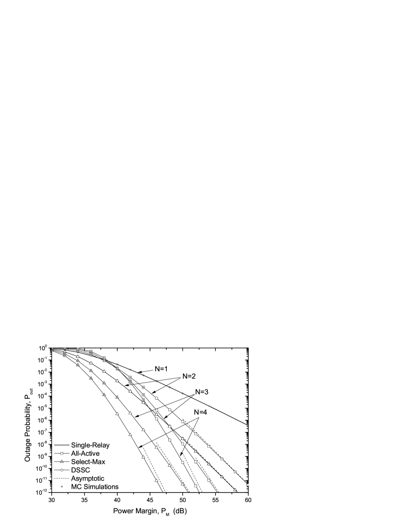
Figure 2: Comparison of relaying protocols for a relay-assisted FSO system with $d_{{}_{SR_{i}}}=d_{{}_{R_{i}D}}=2$ km, $i\in\left\{1,...,N\right\}$.

Fig. 2 depicts the outage performance of the presented relaying protocols for various numbers of relays, when the link distance is identical for all $S$-$R_{i}$ and $R_{i}$-$D$ links and the optical power is equally divided between the active relays. Specifically, analytical results for the outage probability of a relay-assisted FSO system with a link distance of $2$ km are plotted, as functions of the power margin for $N=2,3,4$ relays, using the exact and the asymptotic outage expressions for each of the considered relaying protocols. We assumed $\rho_{{}_{SR_{i}}}=\rho_{{}_{R_{i}D}}=\frac{1}{2N}$ for the all-active and $\rho_{{}_{SR_{i}}}=\rho_{{}_{R_{i}D}}=\frac{1}{2}$ for the select-max and DSSC protocols, respectively. As benchmarks, Monte Carlo (MC) simulation results and the performance of an FSO system with $N=1$, which is independent of the employed relaying protocol, are also illustrated in Fig. 2. As can be observed, there is an excellent match between simulation and analytical results for every value of $N$, verifying the presented theoretical analysis. Moreover, it is obvious that the select-max relaying scheme has a better performance compared to the all-active scheme in every case examined (performance gains of 2, 4, and 5 dB are observed for $N=2$, $3,$ and $4,$ respectively). This result is intuitively pleasing, since the select-max protocol selects in each transmission slot the best end-to-end path out of the $N$ available paths and allocates the total available optical power only to this path. Furthermore, when increasing the number of relays in the select-max and all-active protocols, it is observed that the outage performance is significantly improved with respect to the single relay FSO system. In contrast, although the DSSC scheme with the optimum threshold offers significant performance improvement for $N=2$ (its performance is identical with the select-max performance of $N=2$), it remains unaffected by the increase of the number of relays.

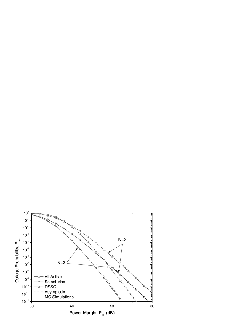
Figure 3: Comparison of relaying protocols for different relay-assisted FSO configurations: $N=2$, $d_{{}_{SR}}=\left\{2,1.5\right\}$, $d_{{}_{RD}}=\left\{1,2.5\right\}$ (in km) and $N=3$, $d_{{}_{SR}}=\left\{2,1.5,1\right\}$, $d_{{}_{RD}}=\left\{1,2.5,3\right\}$ (in km).

Fig. 3 depicts the outage performance of a relay-assisted FSO system employing the presented protocols and assuming different distances for each of the $S$-$R_{i}$ and $R_{i}$-$D$ FSO links. Specifically, two different system configurations are investigated. In the first system configuration, $N=2$ and the link distances are given by vectors $d_{{}_{SR}}=\left\{2,1.5\right\}$ and $d_{{}_{RD}}=\left\{1,2.5\right\}$, with the elements of the vectors respresenting the distances (in km) of the $S$-$R_{i}$ and $R_{i}$-$D$ links respectively, while in the second configuration $N=3$, and the link distances are given by $d_{{}_{SR}}=\left\{2,1.5,1\right\}$ and $d_{{}_{RD}}=\left\{1,2.5,3\right\}$. Fig. 3 reveals that the select-max relaying scheme offers significant performance gains compared to the all-active scheme, also for non-equal link distances. In particular, in the first configuration a gain of 2.5 dB compared to the all-active scheme is offered, while in the second configuration the offered gain is 3 dB. Furthermore, it can be easily observed that although in the second configuration the number of relays has been increased and the performance of both all-active and select-max relaying has been improved, DSSC with optimized threshold remains unaffected by this increase and its performance remains identical with the performance for the first configuration. This was expected, since DSSC uses only two end-to-end paths (those with the minimum end-to-end distance) and, therefore, the addition of extra paths with larger end-to-end distance will not improve the performance of this protocol. Finally, we note that simulation and analytical results are again in excellent agreement.

Fig. 4 illustrates the effect of power allocation in relay-assisted FSO systems employing the relaying protocols under consideration. Specifically, the performaces of the optimum and the proposed sub-optimum power allocation schemes, obtained by solving (62), (65) and from the empirical rules of (63), (69), respectively, are presented along with the equal power allocation, when the second system configuration of Fig. 3 is considered. It is obvious from Fig. 4 that optimized power allocation offers significant performance gains compared to equal power allocation, irrespective of the employed relaying protocol. This was expected, since both the path loss and turbulence strength are distance-dependent in FSO links, and, hence, power allocation schemes that take into consideration the distances of the underlying links, can significantly improve system performance. Furthermore, it is observed that even the simple sub-optimum power allocations schemes lead to substancial performance improvements compared to equal power allocation. Taking into consideration that the parameters for these schemes can be easily obtained, based only on the link distances (for most practical FSO applications, the link distances are fixed and, thus, are known a-priori at both the transmitter and relays), the proposed sub-optimum power allocation can be considered as a less complex alternative to optimum power allocation.

VI Conclusions

We investigated several transmission protocols for relay-assisted FSO systems without direct link between the source and the destination for the Gamma-Gamma channel model. Alternative protocols to the all-active relaying scheme were proposed, which activate only a single relay in each transmission slot. Thus, considerable benefits in terms of implementation complexity are resulted, since the need for synchronizing the relays’ transmissions in order for the FSO signals to arrive simultaneously at the destination is avoided. In particular, two different types of relay selection protocols were proposed: select-max and DSSC. Select-max relaying offers significant performance gains compared to the all-active scheme at the expense of requiring the CSI by all the available links. In contrast, DSSC relaying requires less CSI than select-max (only from the links used in the previous transmission slot), however it exploits only the two relays with the minimum end-to-end distance. Furthermore, based on the derived outage probability expressions, the problem of allocating the power resources to the FSO links was addressed, and optimum and sub-optimum solutions that minimize the system’s outage probability were derived for each considered relaying protocol. Numerical results were provided, which clearly demonstrated the improvements in the power efficiency offered by the proposed power allocation schemes.

Appendix I

Using the infinite series representation of the Gamma-Gamma pdf [21, Eqs. (7), (8)] and since $P_{out,AB}=\int_{0}^{\frac{1}{\bar{h}_{{}_{AB}}\rho_{AB}P_{M}}}f_{\tilde{h}_{{}_{AB}}}\left(x\right)dx$, the outage probability for the FSO link between terminals $A$ and $B$ can be obtained after some basic algebraic manipulations, as

$$P_{out,AB}=\frac{\frac{\pi}{\sin\left(\pi\left(\alpha_{{}_{AB}}-\beta_{{}_{AB}}\right)\right)}}{\Gamma\left(\alpha_{{}_{AB}}\right)\Gamma\left(\beta_{{}_{AB}}\right)}\sum_{l=0}^{\infty}\left(\frac{\frac{1}{l!\left(\beta_{{}_{AB}}+l\right)}\left(\frac{\alpha_{{}_{AB}}\beta_{{}_{AB}}}{\bar{h}_{{}_{AB}}\rho_{AB}P_{M}}\right)^{\beta_{{}_{AB}}+l}}{\Gamma\left(l-\alpha_{{}_{AB}}+\beta_{{}_{AB}}+1\right)}-\frac{\frac{1}{l!\left(\alpha_{{}_{AB}}+l\right)}\left(\frac{\alpha_{{}_{AB}}\beta_{{}_{AB}}}{\bar{h}_{AB}\rho_{AB}P_{M}}\right)^{\alpha_{{}_{AB}}+l}}{\Gamma\left(l+\alpha_{{}_{AB}}-\beta_{{}_{AB}}+1\right)}\right).$$ (70)

For high values of power margin, i.e., $P_{M}\rightarrow\infty$, the term for $l=0$ is dominant and hence (70) can be approximated by

$$P_{out,AB}=\frac{\frac{\pi}{\sin\left(\pi\left(\alpha_{{}_{AB}}-\beta_{{}_{AB}}\right)\right)}}{\Gamma\left(\alpha_{{}_{AB}}\right)\Gamma\left(\beta_{{}_{AB}}\right)}\left(\frac{\left(\frac{\alpha_{{}_{AB}}\beta_{{}_{AB}}}{\bar{h}_{{}_{AB}}\rho_{AB}P_{M}}\right)^{\beta_{{}_{AB}}}}{\Gamma\left(1-\alpha_{{}_{AB}}+\beta_{{}_{AB}}\right)\beta_{{}_{AB}}}-\frac{\left(\frac{\alpha_{{}_{AB}}\beta_{{}_{AB}}}{\bar{h}_{{}_{AB}}\rho_{AB}P_{M}}\right)^{\alpha_{{}_{AB}}}}{\Gamma\left(1+\alpha_{{}_{AB}}-\beta_{{}_{AB}}\right)\alpha_{{}_{AB}}}\right),$$ (71)

which can be reduced to (19), after using the Euler’s reflection formula [18, Eq. (8.334.3)] and introducing $p_{{}_{AB}}$ and $q_{{}_{AB}}$. This concludes the proof.

Appendix II

Based on the infinite series representation of the Gamma-Gamma pdf [21, Eqs. (7), (8)], the pdf of $\xi_{m}=\rho_{{}_{{}_{R_{m}D}}}h_{{}_{R_{m}D}}$ can be written as

$$f_{{}_{\xi_{m}}}\left(x\right)=\frac{\left(\frac{\alpha_{{}_{R_{m}D}}\beta_{{}_{R_{m}D}}}{\bar{h}_{{}_{R_{m}D}}\rho_{{}_{{}_{R_{m}D}}}}\right)^{q_{{}_{R_{m}D}}}\Gamma\left(p_{{}_{R_{m}D}}-q_{{}_{R_{m}D}}\right)}{\Gamma(\alpha_{{}_{R_{m}D}})\Gamma(\beta_{{}_{R_{m}D}})}x^{q_{{}_{R_{m}D}}-1}+O\left(x^{q_{{}_{R_{m}D}}}\right),$$ (72)

where $O\left(\cdot\right)$ represents the least significant terms of an infinite series as $x\rightarrow\infty$. By taking the Laplace transform of the above equation, the MGF expression of $\xi_{m}$ can be obtained as

$$\mathcal{M}_{{}_{\xi_{m}}}\left(s\right)=\frac{\left(\frac{\alpha_{{}_{R_{m}D}}\beta_{{}_{R_{m}D}}}{\bar{h}_{{}_{R_{m}D}}\rho_{{}_{{}_{R_{m}D}}}}\right)^{q_{{}_{R_{m}D}}}\Gamma\left(p_{{}_{R_{m}D}}-q_{{}_{R_{m}D}}\right)}{\Gamma(\alpha_{{}_{R_{m}D}})\Gamma(\beta_{{}_{R_{m}D}})}s^{-q_{{}_{R_{m}D}}}+O\left(s^{-q_{{}_{R_{m}D}}-1}\right).$$ (73)

Hence, the MGF for $h_{{}_{S\left(n\right)}}=\sum\limits_{m\in S\left(n\right)}\rho_{{}_{{}_{R_{m}D}}}h_{{}_{R_{m}D}}$ can be written as

$$\mathcal{M}_{{}_{h_{{}_{S\left(n\right)}}}}\left(s\right)=s^{-\sum\limits_{m\in S\left(n\right)}q_{{}_{R_{m}D}}}\prod\limits_{m\in S\left(n\right)}\frac{\left(\frac{\alpha_{{}_{R_{m}D}}\beta_{{}_{R_{m}D}}}{\bar{h}_{{}_{R_{m}D}}\rho_{{}_{{}_{R_{m}D}}}}\right)^{q_{{}_{R_{m}D}}}\Gamma\left(p_{{}_{R_{m}D}}-q_{{}_{R_{m}D}}\right)}{\Gamma(\alpha_{{}_{R_{m}D}})\Gamma(\beta_{{}_{R_{m}D}})}+O\left(s^{-\sum\limits_{m\in S\left(n\right)}q_{{}_{R_{m}D}}-1}\right).$$ (74)

and, by taking the inverse Laplace transform of (74), an expression for the pdf of $h_{{}_{S\left(n\right)}}$ is obtained as

$$f_{{}_{h_{{}_{S\left(n\right)}}}}\left(x\right)=\frac{\prod\limits_{m\in S\left(n\right)}\left(\frac{\alpha_{{}_{R_{m}D}}\beta_{{}_{R_{m}D}}}{\bar{h}_{{}_{R_{m}D}}\rho_{{}_{{}_{R_{m}D}}}}\right)^{q_{{}_{R_{m}D}}}\frac{\Gamma\left(q_{{}_{R_{m}D}}\right)\Gamma\left(p_{{}_{R_{m}D}}-q_{{}_{R_{m}D}}\right)}{\Gamma\left(\alpha_{{}_{R_{m}D}}\right)\Gamma\left(\beta_{{}_{R_{m}D}}\right)}}{\Gamma\left(\sum\limits_{m\in S\left(n\right)}q_{{}_{R_{m}D}}\right)}x^{\left(\sum\limits_{m\in S\left(n\right)}q_{{}_{R_{m}D}}\right)-1}+O\left(x^{\sum\limits_{m\in S\left(n\right)}q_{{}_{R_{m}D}}}\right)$$ (75)

After some basic algebraic manipulations and keeping only the dominant term, the asymptotic expression in (32) is obtained for the cdf of $h_{{}_{S\left(n\right)}}$. This concludes the proof.

Figure 4: Comparison of power allocation schemes for the relaying protocols under consideration.

References

• [1] H. Willebrand and B. S. Ghuman, Free Space Optics: Enabling Optical Connectivity in Today s Networks.   Sams Publishing, 2002.
• [2] L. Andrews, R. L. Philips, and C. Y. Hopen, Laser Beam Scintillation with Applications.   SPIE Press, 2001.
• [3] X. Zhu and J. M. Kahn, “Performance Bounds for Coded Free-Space Optical Communications through Atmospheric Turbulence Channels,” IEEE Trans. Commun., vol. 51, pp. 1233–1239, Aug. 2003.
• [4] M. L. B. Riediger, R. Schober, and L. Lampe, “Fast Multiple-Symbol Detection for Free-Space Optical Communications,” IEEE Trans. Commun., vol. 57, pp. 1119–1128, Apr. 2009.
• [5] E. Lee and V. Chan, “Part 1: Optical Communication over the Clear Turbulent Atmospheric Channel Using Diversity,” IEEE J. Sel. Areas Commun., vol. 22, pp. 71 896–1906, Nov. 2004.
• [6] S. M. Navidpour and M. Uysal, “BER Performance of Free-Space Optical Transmission with Spatial Diversity,” IEEE Trans. Wireless Commun., vol. 6, pp. 2813–2819, Aug. 2007.
• [7] S. G. Wilson, M. Brandt-Pearce, Q. Cao, and J. H. Leveque, “Free-Space Optical MIMO Transmission with Q-ary PPM,” IEEE Trans. Commun., vol. 53, pp. 1402–1412, Aug. 2005.
• [8] M. Safari and M. Uysal, “Relay-Assisted Free-Space Optical Communication,” IEEE Trans. Wireless Commun., vol. 7, pp. 5441–5449, Dec. 2008.
• [9] M. Kamiri and N. Nasiri-Kerari, “BER Analysis of Cooperative Systems in Free-Space Optical Networks,” IEEE/OSA J. Lightw. Techn., vol. 27, pp. 5639–5647, Dec. 2009.
• [10] ——, “Free-Space Optical Communications via Optical Amplify-and-Forward Relaying,” IEEE/OSA J. Lightw. Techn., vol. 29, pp. 242–248, Jan. 2011.
• [11] C. Abou-Rjeily and A. Slim, “Cooperative Diversity for Free-Space Optical Communications: Transceiver Design and Performance Analysis,” IEEE Trans. Commun., vol. 53, no. 3, pp. 658–663, Mar. 2011.
• [12] T. A. Tsiftsis, G. K. Karagiannidis, P. T. Mathiopoulos, and S. A. Kotsopoulos, “Nonregenerative Dual-Hop Cooperative Links with Selection Diversity,” EURASIP J. Wireless Commun. and Netw., vol. 2006, pp. 1–8, 2006.
• [13] D. S. Michalopoulos and G. K. Karagiannidis, “Two-Relay Distributed Switch and Stay Combining (DSSC),” IEEE Trans. Commun., vol. 56, no. 11, pp. 1790–1794, Nov. 2008.
• [14] D. S. Michalopoulos, A. S. Lioumpas, G. K. Karagiannidis, and R. Schober, “Selective Cooperative Relaying over Time-Varying Channels,” IEEE Trans. Commun., vol. 58, no. 8, pp. 2402–2412, Aug. 2010.
• [15] H. S. Nalwa, Handbook of Organic Electronics and Photonics.   American Scientific Publishers, 2006.
• [16] M. Yano, F. Yamagishi, and T. Tsuda, “Optical MEMS for Photonic Switching-Compact and Stable Optical Crossconnect Switches for Simple, Fast, and Flexible Wavelength Applications in Recent Photonic Networks,” IEEE J. Sel. Topics Quantum Electron., vol. 11, pp. 383–194, 2005.
• [17] X. Zhu and J. M. Kahn, “Free-Space Optical Communication through Atmospheric Turbulence Channels,” IEEE Trans. Commun., vol. 50, no. 8, pp. 1293–1300, Aug. 2002.
• [18] I. S. Gradshteyn and I. M. Ryzhik, Table of Integrals, Series, and Products, 7th ed.   Academic, 2007.
• [19] M. A. Al-Habash, L. C. Andrews, and R. L. Philips, “Mathematical Model for the Irradiance Probability Density Function of a Laser Beam Propagating through Turbulent Media,” Opt. Engineering, vol. 40, pp. 1554–1562, Aug. 2001.
• [20] T. A. Tsiftsis, “Performance of Heterodyne Wireless Optical Communication Systems over Gamma-Gamma Atmospheric Turbulence Channels,” Electron. Lett., vol. 44, Feb. 2008.
• [21] E. Bayaki, R. Schober, and R. Mallik, “Performance Analysis of MIMO Free-Space Optical Systems in Gamma-Gamma fading,” IEEE Trans. Commun., vol. 57, no. 11, pp. 1119–1128, Nov. 2009.
• [22] M. K. Simon and M. S. Alouini, Digital communications over Fading Channels.   Wiley Interscience, 2005.
• [23] P. S. Bithas, N. C. Sagias, P. T. Mathiopoulos, G. K. Karagiannidis, and A. A. Rontogiannis, “On the Performance Analysis of Digital Communications over Generalized-$K$ Fading Channels,” IEEE Commun. Lett., vol. 10, pp. 353–355, May 2006.
• [24] A. Papoulis and S. U. Pillai, Probability, Random Variables and Stochastic Processes, 4th ed.   Mc Graw Hill, 2002.
• [25] M. O. Hasna and M.-S. Alouini, “Optimal Power Allocation for Relayed Transmissions Over Rayleigh-Fading Channels,” IEEE Trans. Wireless Commun., vol. 3, no. 6, pp. 1999–2004, Nov. 2004.
• [26] J. Nocedal and S. J. Wright, Numerical Optimization.   Springer, 1999.
• [27] B. Anderson, J. Jackson, and M. Sitharam, “Descartes’ rule of sign revisited,” The American Mathematical Monthly, vol. 105, no. 5, pp. 447–451, May 1998.
Refer to caption