Effects of many-electron jumps in relaxation and conductivity of Coulomb glasses

Abstract

A numerical study of the energy relaxation and conductivity of the Coulomb glass is presented. The role of many-electron transitions is studied by two complementary methods: a kinetic Monte Carlo algorithm and a master equation in configuration space method. A calculation of the transition rate for two-electron transitions is presented, and the proper extension of this to multi-electron transitions is discussed. It is shown that two-electron transitions are important in bypassing energy barriers which effectively block sequential one-electron transitions. The effect of two-electron transitions is also discussed.

I Introduction

At low temperatures, disordered systems with localized electrons (e. g. on dopants of compensated doped semiconductors or Anderson localized states in disordered samples) conduct by phonon assisted hopping. The theory of this process goes back to Mott mott who invented the concept of variable range hopping. In particular he derived the Mott law for the temperature dependence of the conductance

$$\sigma\sim e^{-(T_{0}/T)^{1/(d+1)}}$$

where $d$ is the dimensionality of the sample. If Coulomb interactions are important one describes the system as a Coulomb glass due to the slow dynamics at low temperatures. As is well known (See Ref. ES, and references therein), the single particle density of states develops a soft gap at the Fermi level, the so called Coulomb gap. While this understanding of the density of states is generally accepted, the situation is less clear when it comes to describing dynamics in the interacting case. Using the Coulomb gap density of states, which is a result of interactions, in the variable range hopping argument, assuming that it can be used in the same way as the non-interacting density of states, yields the Efros-Shklovskii law for conductance

$$\sigma\sim e^{-(T_{0}/T)^{1/2}}.$$

While this has been observed experimentally in several cases it is not always the case. It remains clear that this is an uncontrolled approximation, and the full theoretical understanding of this is still missing.

In particular, since this approach is based on a single-particle approximation, it neglects the possibility of correlated jumps of two or more electrons. At low temperatures, the system can be trapped in metastable configurations, from which it can be difficult to escape by single-electron transitions. By a two-electron transition the system can jump out of this metastable state even when the temperature is so low that the probability of making the same transition sequentially is very small because it passes through an activated intermediate state with higher energy. Thus, one would expect the importance of many-electron jumps to increase as the temperature is decreased. This was also the conclusion of some works tenelsen ; pg which used a method which identifies the full set of low energy states of the system, and studies the possible transitions between them. Because the number of accessible states grows rapidly with increasing temperature and system size, this method is restricted to small systems and low temperatures.

The importance of many-electron jumps was disputed by Tsigankov and Efros tsigankov , who used a kinetic Monte Carlo method to study the dynamics of the Coulomb glass. Using only one-electron transitions, they confirm the Efros-Shklovskii law both regarding the value $\frac{1}{2}$ in the exponent and also the value of $T_{0}$ predicted by percolation theoryES . Including two-electron transitions, they find that the two-electron jumps contribute about two orders of magnitude less to the current than the one-electron jumps. Furthermore, they find that the relative contribution of two-electron jumps decreases with decreasing temperature. They conclude that two-electron jumps are not important for the conductance of the Coulomb glass, contradicting the previous works tenelsen ; pg . We do not understand how their results can lead to this conclusion, since the two-electron jumps can be crucial in facilitating transport through one-electron jumps, even if their actual number is much less than the number of one-electron jumps. What should be compared is the conductance when only allowing one-electron jumps with the conductance when two-electron jumps are also included. This will be discussed in more detail later.

Tsigankov and Efros tsigankov explain their contradiction with the previous works tenelsen ; pg as coming from two sources: First, in Ref. pg, the rates of two-electron transitions were overestimated because they were assumed to be independent of the distance between the two electrons involved in the transition. This assumption is not reasonable, since it is the Coulomb interaction which allows the remote electrons to exchange energy, and the probability of a double jump should decrease with distance. Second, the method of identifying the full set of low energy states used in Refs. tenelsen, ; pg, is numerically costly, and therefore limited to very small samples and low temperatures (where only the states with the very lowest energies are thermally excited). Therefore the conclusions of Refs. tenelsen, ; pg, may be the result of small sizes and not valid for larger systems. An attempt to answer the second criticism was made in Ref. somoza, where the size dependence was studied and a scheme for extrapolation to infinite size was suggested. Using the same percolation method in configuration space as in Ref. pg, (including the same expression for the many-electron transition rate which was questioned in Ref. tsigankov, ) it was still found that many-electron jumps become important at low temperatures. The difference with the results of Ref. tsigankov, is explained by the fact that the method they used, studying all transitions between an extensive set of low energy states and involving up to six electrons moving together, was more suited to identify the crucial many-electron transitions. These could enhance the conductance even if they happen only very rarely since they could facilitate subsequent one-electron transitions. Since the Monte Carlo methodtsigankov becomes impracticably slow at low temperatures while the percolation in configuration spacepg ; somoza only can be applied for small systems and low temperatures, several questions remained unanswered: Is the difference in the expression for the many-electron transition rate the reason for the difference in results? Are the two methods equivalent, or does one of them contain systematic errors? At what temperatures are the many-electron transitions important?

In this work we try to answer these questions. Previous works have focused on the influence of multi-electron transitions on conductance since this is the commonly measured quantity. However, at low temperatures it can be difficult to numerically find the conductance for two reasons: First, the system should be equilibrated which is a slow process at low temperatures. Second, to be in the linear response regime one must use a small potential difference across the sample, and the resulting current is so weak that one needs a long sampling time to get accurate values. Therefore we have chosen to study the relaxation of energy instead, this being a quantity easily accessible in simulations. It is also well known that experimentallyzvi ; grenet the conductance is also slowly relaxing, so that relaxation may be as important and relevant as equilibrium conductance (Although one should keep in mind that the experiments of Ref. grenet, are on granular aluminium films, and it may be that this system is more complex than the model discussed here accounts for). This allows us to go to lower temperatures using the Monte Carlo method, and thereby bridge the gap to the configuration space method. Here we report on the following: We give a direct calculation of the transition rate for two-electron jumps, to replace the unphysical one used in Refs. pg, ; somoza, and the approximate one suggested in Ref. tsigankov, . A preliminary report of this part of our work was already presented in Ref. BeSo09, . We also discuss the extension of this result to many-electron transitions (Sec. II). We have numerically studied the relaxation of the total energy of the system, comparing the evolution when only allowing one-electron jumps with the one where two- and three-electron jumps are included. We have used both the Monte Carlo algorithm suggested by Tsigankov and Efrostsigankov and the configuration space method of Refs. pg, ; somoza, , but instead of using the percolation method we have studied the master equation on the set of low energy states, thereby eliminating any doubt on the accuracy of the percolation method. The details of the models used and the numerical procedures are given in Sec. III. The results on energy relaxation are presented in Sec. IV and some results on conductance in Sec. V.

II Many-electron transition rates

We start from the standard Coulomb gap Hamiltonian with a perturbation term due to tunneling

$$H_{0}=\sum_{i}\phi_{i}c_{i}^{\dagger}c_{i}+\sum_{i<j}V_{ij}c_{i}^{\dagger}c_{i}c_{j}^{\dagger}c_{j}+\sum_{i<j}t_{ij}c_{i}^{\dagger}c_{j}+\mbox{h.c.}$$ (1)

describing localized electrons interacting through Coulomb forces. $c_{i}^{\dagger}$ and $c_{i}$ are operators creating and annihilating an electron on site $i$, $\phi_{i}$ is the intrinsic energy of site $i$, which we assume to be a random variable uniformly distributed in the interval $[-W/2,W/2]$, and $V_{ij}=e^{2}/{r_{ij}}$ is the Coulomb energy. The tunneling amplitude $t_{ij}=I_{0}e^{-2r_{ij}/a}$ depends exponentially on the distance $r_{ij}$, and $a$ is the localization radius and the prefactor is $I_{0}=e^{2}/\kappa a$ with $\kappa$ the dielectric constant.

We consider phonon assisted tunneling due to the electron-phonon interaction:

$$H_{\text{e-ph}}=\sum_{\bf q}\sum_{i}c_{i}^{\dagger}c_{i}\left(e^{-i{\bf qr}_{i}}\gamma_{\bf q}b_{\bf q}+\mbox{h.c.}\right)$$ (2)

where $b_{\bf q}$ is the phonon annihilation operator and $\gamma_{\bf q}$ is a numerical factor depending on the exact phonon interaction.

The one-electron transition rate from site $i$ to site $j$ is well known, see for example Ref. ES, ,

$$\Gamma_{ij}\propto|\gamma_{q}|^{2}N(\Delta E)e^{-2r_{ij}/a}$$

where $r_{ij}$ is the distance between the sites and $\Delta E$ is the change in energy. $N(E)=1/(e^{E/T}-1)$ is the equilibrium phonon density, for emmision processes this has to be replaced by $N(E)+1$. We set $k_{B}=1$ so that temperatures and energies are measured in the same units. In this work, following Ref. tenelsen, we use the formula

$$\Gamma_{ij}={\tau_{0}}^{-1}e^{-2r_{ij}/a}\min\left(e^{-\Delta E/T},1\right)$$

where $\tau_{0}$ contains material dependent factors and energy dependent factors, which we approximate by their average value; we consider it as constant and its value, of the order of $10^{-12}$ s is chosen as our unit of time (Note that in Ref. tsigankov, a different formula was used, we do not believe that the difference is of great significance, although it may change numerical values).

II.1 Two electron transition rates

Let us concentrate for the moment in transitions of two electrons on four sites and follow the method described in Ref. BeSo09, , based on the locator expansion in configuration space. We can restrict ourselves to the four sites involved in the transition and include the Coulomb interaction with the rest of the system in the site energy $\phi_{i}$. The zero-order (in the tunneling perturbation) configurations of two electrons on four sites are described by the states

$$|\;\!_{\circ}^{\bullet}\;\!{}_{\circ}^{\bullet}\rangle\quad|\;\!_{\bullet}^{\bullet}\;\!{}_{\circ}^{\circ}\rangle\quad|\;\!_{\circ}^{\bullet}\;\!{}_{\bullet}^{\circ}\rangle\quad|\;\!_{\bullet}^{\circ}\;\!{}_{\circ}^{\bullet}\rangle\quad|\;\!_{\circ}^{\circ}\;\!{}_{\bullet}^{\bullet}\rangle\quad|\;\!_{\bullet}^{\circ}\;\!{}_{\bullet}^{\circ}\rangle$$ (3)

where filled circles represent sites with electrons and empty circles empty sites. The sites are numbered as $|\;\!_{3}^{1}\;\!{}_{4}^{2}\rangle$. We calculate the initial and the final states to second order in the tunneling, and we denote them by $|\widetilde{\;}\!_{\circ}^{\bullet}\;\!{}_{\circ}^{\bullet}\rangle$ to $|\widetilde{\;}\!_{\bullet}^{\circ}\;\!{}_{\bullet}^{\circ}\rangle$.

We consider phonon assisted tunneling from the initial perturbed state $|\widetilde{\;}\!_{\circ}^{\bullet}\;\!{}_{\circ}^{\bullet}\rangle$ to the final state $|\widetilde{\;}\!_{\bullet}^{\circ}\;\!{}_{\bullet}^{\circ}\rangle$. The calculation is a direct generalization of the one found in Ref. ES, for one-electron transitions. We assume that the electron on an impurity is described by a hydrogen-like wavefunction with a localization radius $a$ and that $qa\ll 1$ where $q$ is the wave vector of the phonon, so that

$$\langle i|e^{-i{\bf qr}_{i}}|i\rangle\approx e^{-i{\bf qr}_{i}}$$ (4)

where $|i\rangle$ describes an electron on impurity $i$. After some algebra we find

$$M_{\bf q} =\langle\widetilde{\;}\!_{\circ}^{\bullet}\;\!{}_{\circ}^{\bullet}|\sum_{i}e^{-i{\bf qr}_{i}}c_{i}^{+}c_{i}|\widetilde{\;}\!_{\bullet}^{\circ}\;\!{}_{\bullet}^{\circ}\rangle=t_{13}t_{24}\frac{E_{\;\!{}_{\bullet}^{\circ}\;\!{}_{\bullet}^{\circ}}-E_{\;\!{}_{\bullet}^{\circ}\;\!{}_{\circ}^{\bullet}}+E_{\;\!{}_{\circ}^{\bullet}\;\!{}_{\circ}^{\bullet}}-E_{\;\!{}_{\circ}^{\bullet}\;\!{}_{\bullet}^{\circ}}}{E_{\;\!{}_{\bullet}^{\circ}\;\!{}_{\bullet}^{\circ}}-E_{\;\!{}_{\circ}^{\bullet}\;\!{}_{\circ}^{\bullet}}}$$ (5)

$$\left[\frac{e^{-i{\bf qr}_{1}}-e^{-i{\bf qr}_{3}}}{(E_{\;\!{}_{\circ}^{\bullet}\;\!{}_{\circ}^{\bullet}}-E_{\;\!{}_{\circ}^{\bullet}\;\!{}_{\bullet}^{\circ}})(E_{\;\!{}_{\bullet}^{\circ}\;\!{}_{\bullet}^{\circ}}-E_{\;\!{}_{\bullet}^{\circ}\;\!{}_{\circ}^{\bullet}})}+\frac{e^{-i{\bf qr}_{2}}-e^{-i{\bf qr}_{4}}}{(E_{\;\!{}_{\circ}^{\bullet}\;\!{}_{\circ}^{\bullet}}-E_{\;\!{}_{\bullet}^{\circ}\;\!{}_{\circ}^{\bullet}})(E_{\;\!{}_{\bullet}^{\circ}\;\!{}_{\bullet}^{\circ}}-E_{\;\!{}_{\circ}^{\bullet}\;\!{}_{\bullet}^{\circ}})}\right]$$

$E_{\alpha}$ refers to the energy of configuration $|\alpha\rangle$. This expression corresponds to electrons jumping from site 1 to 3 and 2 to 4. We have to add a similar expression involving the jump from 1 to 4 and from 2 to 3. If the sites are at random positions, the jump with the minimum total hopping distance will dominate and we can neglect the other jumping possibilities, but if the sites are on a lattice we have to keep all the terms (and their cross terms) in the calculation of $|M_{\bf q}|^{2}$.

We further assume that $qr_{ij}\gg 1$ (this may fail at sufficiently low temperatures), which allows us to replace factors of the form $\cos{\bf qr}_{ij}$, appearing in matrix elements of wavefunctions of different sites, by 0 when integrating over the directions of ${\bf q}$. Let us concentrate on the different energy factors appearing in Eq. (5). We first note that $E_{\;\!{}_{\bullet}^{\circ}\;\!{}_{\bullet}^{\circ}}-E_{\;\!{}_{\circ}^{\bullet}\;\!{}_{\circ}^{\bullet}}=\Delta E$ is the total energy difference and will be equal to the energy of the phonon that is emitted or absorbed which then determines the phonon wave vector. Further,

$$E_{\;\!{}_{\bullet}^{\circ}\;\!{}_{\bullet}^{\circ}}-E_{\;\!{}_{\bullet}^{\circ}\;\!{}_{\circ}^{\bullet}}+E_{\;\!{}_{\circ}^{\bullet}\;\!{}_{\circ}^{\bullet}}-E_{\;\!{}_{\circ}^{\bullet}\;\!{}_{\bullet}^{\circ}}\sim V_{12}+V_{34}-V_{14}-V_{23}\equiv V_{13,24}$$ (6)

is independent of the site energies. It only depends on the geometrical disposition of the jumps and if the separation between sites of different jumps is much larger than both jumping distances it corresponds to the dipole-dipole interaction. The energy denominators in Eq. (5) involve the intermediate states, and it is very CPU time consuming to calculate these terms in numerical simulations. The divergence of these terms at certain points reflect the limitation of the perturbation theory rather than any physical effect. Therefore we want to cut off this divergence and replace the fraction by 1 when it is larger than 1. The energy differences are of the order of the disorder $W$. Therefore the terms in the brackets are also never very small. Since they are also temperature independent we propose to set these terms equal to $1/W$. We believe that this is of no physical consequence, and will not affect the results qualitatively. Taking into account these approximations and using Fermi’s golden rule we arrive at the expression for the transition rate

$$\Gamma_{\;\!{}_{\circ}^{\bullet}\;\!{}_{\circ}^{\bullet}\rightarrow\;\!_{\bullet}^{\circ}\;\!{}_{\bullet}^{\circ}}=\tau_{0}^{-1}\frac{I_{0}^{2}V_{13,24}^{2}}{(W/2)^{4}}e^{-2(r_{13}+r_{24})/a}\min\left(e^{-\Delta E/T},1\right)$$ (7)

where $\tau_{0}$ is the same unit of time as for one-electron transitions and we assume that the average energy difference of intermediate states is W/2. More details on the derivation of this equation were given in Ref. BeSo09, .

II.2 Three and more electron transition rates

In this case one has to assume that the interaction is weak and do perturbation theory in both the interaction and the hopping term. As for two-electron jumps, it is an excellent approximation for sites at random to consider only the transitions with the minimum total hopping distance $R_{I,J}$. There are many of them, differing in the order of the one electron moves and on the jump directly excited by the phonon. The final expression for the transition rate is very complex, but its most important factor is easy to get (Po81, ). It is the probability of finding a phonon of energy $\Delta E$ times the product of the overlap integrals of the hops of all electrons involved in the transition. The many electron transition rate can then be approximated by

$$\Gamma_{I,J}=\tau_{0}^{-1}\gamma^{n-1}e^{-{2R_{I,J}}/{a}}\min\left(e^{-\Delta E/T},1\right).$$ (8)

$\gamma$ is a measure of the importance of the interaction energy compared to the disorder energy and $n$ is the number of electrons participating in the process.

The use of equation (8) for the transition rates in numerical simulations may overestimate the importance of correlated hops since it doublecounts the effects of excitations well separated one from each other. Although one-electron excitations should dominate in this case, since many-electron excitations should only be important when single excitations have positive energies, while the combined excitation has negative energy, it is convenient to get rid of this problem. We can do that by substituting the constant $\gamma$ by a prefactor similar to the one obtained for two-electron transitions, equation (7). It is difficult to get a closed expression for this prefactor, and we propose an empirical approach that it is practical for numerical purposes and that we think incorporates the relevant physics of the problem. A requirement for this prefactor is that it should vanish when one of the transitions is very far from the others. A suggestion satisfying this requirement is the sum of all the products of $n-1$ different interaction energies between any pair of single electron transitions, like $V_{13,24}$ in (6). Each of these terms must be divided by a factor proportional to the disorder energy as in the two-electron case. This proposal corresponds to exciting one of the hops by the phonon and the rest by the dipole-dipole interaction in all the possible ways. For three electron transitions we take as the preexponential

$$\frac{I_{0}^{2}}{\tilde{W}^{6}}(V_{14,25}^{2}V_{25,36}^{2}+V_{25,36}^{2}V_{14,36}^{2}+V_{14,25}^{2}V_{14,36}^{2}).$$ (9)

III Model for numerical simulations

We use the standard tight–binding Coulomb gap Hamiltonian ES :

$$H=\sum_{i}\epsilon_{i}n_{i}+\sum_{i<j}{\frac{(n_{i}-K)(n_{j}-K)}{r_{ij}}}\;,$$ (10)

$K$ being the compensation. We take the number of electrons to be half the number of sites. The sites are arranged in two dimensions both on a lattice and at random, but in the latter case with a minimum separation between them, which we choose to be $0.05r$ where $r^{2}=L^{2}/N$. We implement cyclic boundary conditions in both directions. We take $e^{2}/r$ as our unit of energy and $r$ as our unit of distance.

III.1 Monte Carlo algorithm for lattice systems

For the two-electron transition rate we use Eq. (7) for sites at random and the extension that includes the two jumping possibilities when sites are on a lattice. As for one-electron transitions, the rate is split in one energy dependent (or activation) term, $\Gamma^{A}$ and one distance dependent (or tunneling) term $\Gamma^{T}$. This means that we can use the hybrid algorithm of Tsigankov and Efros tsigankov .

The program first calculates and stores the distance dependent part of the rates. For the one electron jumps, the tunneling parts of the rate for all jumps in the square $|\Delta x|,\;|\Delta y|\leq L_{1}$ some maximal jump length (in the numerics $L_{1}=10$ lattice units) are calculated. The sum $\Gamma_{T,1}^{Total}=\sum\Gamma_{T,1}$ is also stored. For the two electron jumps, all coordinates are relative to the initial position of the first electron. The following algorithm is used:

• The final position of the first electron is selected in the square $|\Delta x|,\;|\Delta y|\leq L_{2}$ where the size $L_{2}$ can be reasonably chosen to be about half of $L_{1}$ since the distances each electron jumps are added together to find the rate (In the numerics $L_{2}=3$ lattice units).

• The initial position of the second electron is selected in the square $|x_{2}|,\;|y_{2}|\leq D_{2}$ (In the numerics $D_{2}=5$ lattice units). The initial position of the second electron can not be either the initial or the final position of the first electron.

• The final position of the second electron is selected in the square $|\Delta x_{2}|,\;|\Delta y_{2}|\leq L_{2}$. The final position of the second electron can not be the initial or final position of the first electron.

• The tunneling part of the rate for this transition is calculated according to the formula

  $$\Gamma_{T,2}=E_{1}^{2}V_{13,24}^{2}+E_{2}^{2}V_{14,23}^{2}+E_{1}E_{2}V_{13,24}V_{14,23}$$

  where

  $$E_{1}=e^{-2(r_{13}+r_{24})/a},\qquad E_{2}=e^{-2(r_{14}+r_{23})/a}$$

• The rates for all these transitions are stored, and the sum of all $\Gamma_{T,2}^{Total}=\sum\Gamma_{T,2}$ is calculated.

When the Monte Carlo algorithm is running, it will do the following steps in order to select which transition to make.

• It is decided whether to attempt a one electron transition (probability $\Gamma_{T,1}^{Total}/(\Gamma_{T,1}^{Total}+\Gamma_{T,2}^{Total})$) or a two electron transition (probability $\Gamma_{T,2}^{Total}/(\Gamma_{T,1}^{Total}+\Gamma_{T,2}^{Total})$)

• If it is a one electron transition we follow the usual procedure of Tsigankov and Efrostsigankov . One occupied site is selected randomly. Then the final site is selected at random but with weights given by the probability $\Gamma_{T,1}/\Gamma_{T,1}^{Total}$. If the final site is occupied, the transition is rejected. If it is empty it is accepted with probability $\min(1,e^{-\Delta E/T})$.

• If it is a two electron transition an occupied site is selected at random. Then a certain two electron jump is selected weighted by the probability $\Gamma_{T,2}/\Gamma_{T,2}^{Total}$. If the final site of the first electron is occupied, the initial site of the second electron is empty or the final site of the second electron is occupied, the transition is rejected. If not, the transition is accepted with probability $\min(1,e^{-\Delta E/T})$.

III.2 Master equation method for sites at random

We used a numerical algorithm to obtain the ground state and $\approx 10^{5}$ lowest energy many–particle configurations of the system. The algorithm is an improved version of the algorithm in Ref. somoza, and it was described in detail in ds, . It consists of the following two stages. In the first stage, we repeatedly start from states chosen at random and relax each sample by means of a local search procedure. In an iterative process, we look for neighbors of lower energies and always accept the first such state found. The procedure stops when no lower energy neighboring states exist, which insures stability with respect to all one–electron jumps and compact two–electron jumps. We then consider a set of metastable sates found by the process just described and look for the sites which present the same occupation in all of them. These sites are assumed to be frozen, i.e. they are not allowed to change occupation, and the relaxation algorithm is now applied to the unfrozen sites. The whole procedure is repeated until no new frozen sites are found with the set of metastable states considered.

In the second stage, we complete the set of low–energy configurations by generating all the states that differ by one– or two–electron transitions from any configuration stored. In order to speed up this process, which is very CPU time consuming, we again assume frozen and unfrozen sites and in first place look for neighboring configurations by changing the occupation of unfrozen sites only. We later relax this restriction in the final stage.

We consider 20 different realizations of a system with 500 sites. We obtain the 200 000 lowest energy configurations for each realization. We then obtain all one- two- and three electron transitions between all these configurations, establishing a dynamical matrix that evolves the system in time according to this master equation. We choose for the initial state the mixture of all configurations with weights equal to the Boltzmann factor for a temperature 40 times larger than the real one.

We have developed a renormalization procedure to propagate in time efficiently. It takes advantage of the fact that the distribution of relaxation times is exponentially broad and at large times the short time processes must have already equilibrated some sets of configurations. At a given time, we calculate the current through each transition and if it is very small, relative to the transition rate and the occupation probability, we assume that the two configurations involved are in thermal equilibrium and can consider then as part of a cluster. We recalculate the transition rates between this new cluster and the rest of the system. The time step used in the numerical propagation is calculated dynamically and increases drastically as we form more clusters or larger clusters.

IV Results on energy relaxation

IV.1 Relaxation using Monte Carlo on the lattice model

To see the effect of two electron transitions on relaxation we did the following. For one sample of size $100\times 100$ and $W=2$ we ran relaxation from an initial random state at three different temperatures, $T$ = 0.01, 0.005 and 0.001. For each temperature we ran from the same initial state 10 (20 for $T=0.001$) different time evolutions (different random seeds for the Monte Carlo evolution). For each case we ran the simulation both allowing only one electron transitions and including one and two electron transitions.

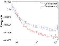
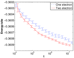
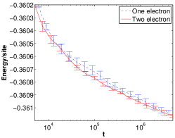
a) b) c)

Figure 1: (Color online) Energy relaxation as function of time at a) $T=0.001$, b) $T=0.005$ and c) $T=0.01$. Averages are shown for one and two electron transitions, error bars are standard deviation of the mean.

The results are shown in Fig. 1. It is clear that as the temperature decreases, the difference between the relaxation rates in the one- and two-electron cases increases. To confirm that the results are general and the sample sufficiently large we did one set of 10 time evolutions on the same sample but starting from a different initial state and one set on a different sample. The same behaviour was seen in all cases.

To see more clearly the importance of the two electron jumps we can look at one particular relaxation graph and mark the points where two electron jumps occur (Figure 2, the two graphs, Figure 2a) and Figure 2b) correspond to two different Monte Carlo evolution of the same sample and initial state).

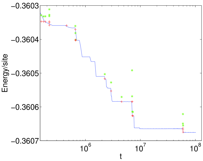
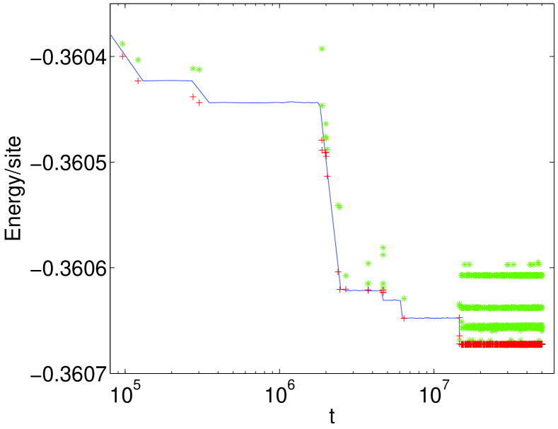
a) b)

Figure 2: (Color online) The correlation between the points where two electron jumps occur and steps in the energy relaxation graph. The blue curve is the total energy of the system. The red points (+) are the final energies after two electron jumps and the green points (*) the energy of the intermediate state if this jump was to be replaced by sequential one electron jumps. $T=0.001$. The two graphs, a) and b), correspond to two different Monte Carlo evolution of the same sample and initial state

In the figure the curve is the energy, while the points mark the time when a two electron jump was performed. The red points represent the final energy after the transition, while the green points represent the energy of the intermediate state if this jump was to be replaced by sequential one electron jumps. The temperature was $T=0.001$, and as we can see the increase in energy to the intermediate state is sometimes more than two orders of magnitude larger that this. This means that the probability of this process occurring sequentially is extremely small. As can be seen from the figure, there are clear correlations between the occurrence of two electron jumps and steps in the relaxation graph. This means that the two electron jumps are essential in overcoming barriers in the relaxation path and give a contribution to the relaxation rate even if the number of two electron jumps can be a small fraction of the total number of jumps. Sometimes (at long times in Fig 2b) there can occur soft two electron excitations which are then jumping back and forth between the two configurations like soft dipoles in the one electron case. These give large contributions if we try to count the number of two electron transitions, but are not important for relaxation.

To better measure the importance of the two electron jumps on the relaxation, we do the following. For each decade in time we see how much the energy was reduced in the two electron jumps (or by one electron jumps immediately following a two electron jump) and compare this to the total relaxation of energy during this time. We then get Fig. 3 and as we can see, the two electron jumps increase in their importance for relaxation, and at the later times in the simulation, they are responsible for most of the relaxation. At long times the fraction slightly exceeds 1 which is due to the fact that the energy of the system was not stored after each jump so the energy reduction in a two electron jump can be slightly overestimated if it was preceeded by one electron jumps which increased the energy.

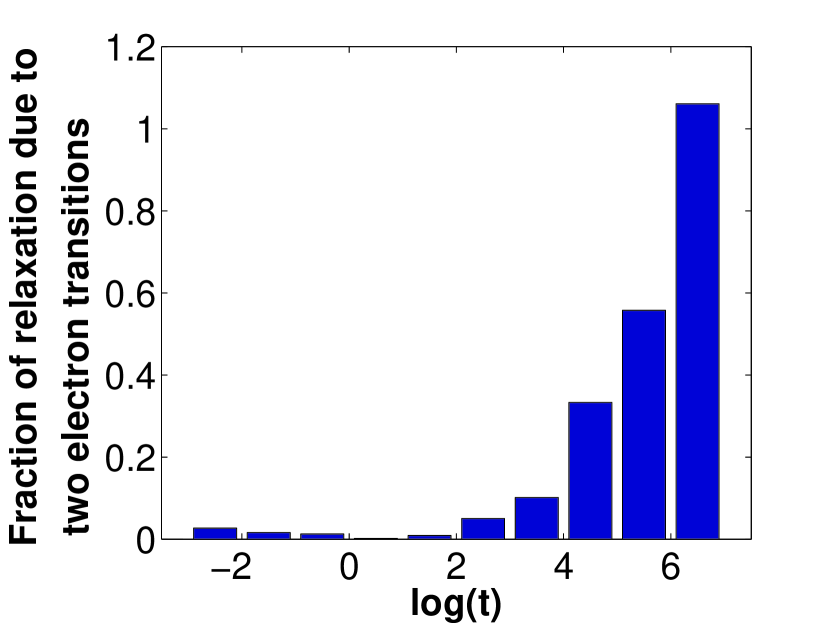
Figure 3: The fraction of relaxation due to two electron transitions. The figure is an average over 6 different Monte Carlo evolutions on one sample at $T=0.001$.

IV.2 Relaxation using master equation on the random sites model

We have calculated the average energy, with respect to the ground state energy, as a function of time. In Figure 4 we plot the results for one-electron and two-electron relaxations at a temperature $T=0.002$ for a system with 500 sites. We consider this small size in order to have configurations extending over a relatively large energy range. The dotted line is the result when only one-electron relaxation is considered. The continuous and the dashed curves correspond to relaxation by one- and two-electron jumps. In the dashed case we have not included any prefactor in the expression for the transition rates, while in the continuous curve we use Eq. (7). We first note how relaxation by one-electron jumps alone is far from complete. The system gets easily stuck in metastable states even for the relatively small system size considered. The inclusion of two-electron jumps is almost negligible at short times, where one can always lower the energy by one-electron jumps. But at larger times, two-electron transitions are really needed to overcome the energy barriers.

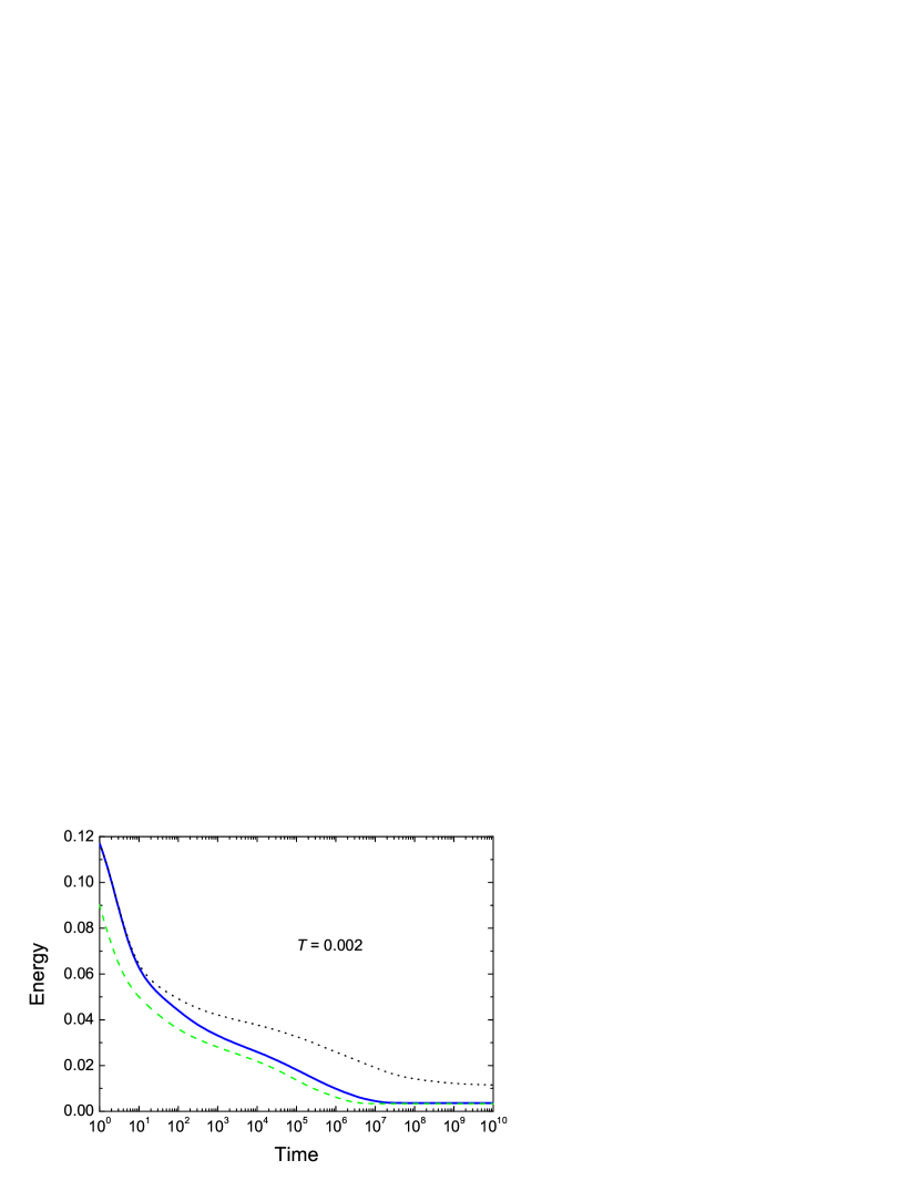
Figure 4: (Color online) Energy relaxation as function of time for one-electron jumps (black dotted curve), one- and two-electron jumps without any prefactor (green dashed curve) and with the prefactor of Eq. (7) (blue continuous curve).

We also note that if we do not include the right prefactor in the two-electron rate we are overestimating their effects, specially at short relaxation times, because we are double counting some excitations. We have checked that the results for two-electron contributions do not change if we only include those transitions with negative interaction energy. This result in an important reduction in the number of many-electron excitations to include in the simulations. In future calculations of many-electron effects it will be convenient to take advantage of this result and to explore more drastic reductions in the number of relevant excitations.

At a time of roughly $10^{7}\tau_{0}$ we have already practically reached the thermal equilibrium when up to two-electron transitions are considered. We expect this time to increase drastically with system size. In figure 5 we have represented energy relaxation by one-electron jumps (dotted curve), by up to two-electron hops (dashed curve) and by up to three-electron jumps (continuous curve). For three-electron jumps we have used for the prefactor the sum of all the different products of dipole-dipole contributions. We note that the inclusion of three-electron jumps does not affect much the results for the size considered. We expect that their effects will be more important for larger sizes, which will contain larger energy barriers and a more complex energy landscape. As we include transitions of more particles, the energy relaxation curve seems to approach a logarithmic behavior.

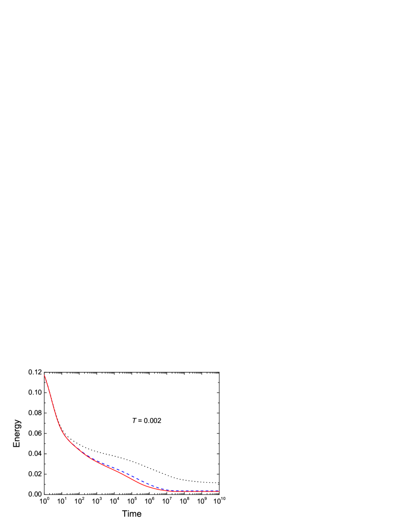
Figure 5: (Color online) Energy relaxation as function of time for one-electron jumps (black dotted curve), one- and two-electron jumps (blue dashed curve) and up to three-electron jumps (red continuous curve).

V Results on conductivity

We also studied conductivity, comparing the cases with and without two electron jumps. At temperatures $T\geq$ 0.04 we ran four different samples of size 100$\times$100. For $T\leq$ 0.04 we used four samples of size 200$\times$200 (this because we know that at low temperatures we see finite size effects in the conductance up to $L=100$). The electric field was $T/10$, which should be in the ohmic regime. In each case we ran the simulation for $10^{7}$ accepted jumps and checked that this was sufficient to obtain a straight line of transferred charge as function of time. The conductance is then given by the slope of this line. The results are shown in Fig. 6.

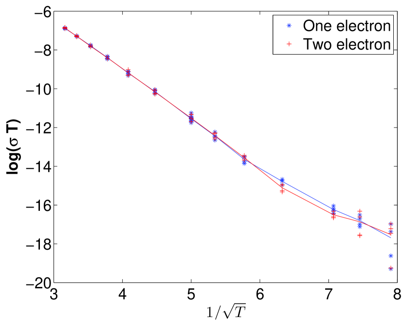
Figure 6: (Color online) Conductance as function of temperature showing the Efros Shklovskii law. Blue points (*) are with one electron jumps, red points (+) include also two electron jumps. Four samples are shown for each temperature, the spread indicates the uncertainty. The lines are the averages.

We see that we reproduce the Efros-Shklovskii law for the conductivity and that there is no significant difference when including two-electron transitions.

VI Discussion

Comparing our results with the previous works pg ; tsigankov ; somoza it seems that all fall into the same coherent picture. By focusing on relaxation, we were able to apply the Monte Carlo method to temperatures comparable to the ones were the master equation approach can be used. Then we see similar behavior in both the cases. The energy relaxes faster when two electron transitions are included. A more direct comparison of the two methods is difficult since the models differ in several respects. In the Monte Carlo method we prefer to use a lattice since it reduces the computational effort while in the master equation we are resticted to small samples and prefer a random site model since we believe that lattice effects are more severe for small systems. Also, the initial states are different in the two cases, since in the master equation approach we need to take as initial state some combination of the states in the low-energy set we are working on. These are already very low-energy states, and different in structure from the random states used in the Monte Carlo method. However, we find that our results convincingly show that both methods give similar results at low temperatures, and that there are no systematic errors which affect one or the other method. Furthermore, if we look at Figure 4 and compare the two graphs including two electron transitions, with and without the prefactor in Eq. (7), we find that although the omission of the prefactor overestimates the importance of two electron jumps the results remain qualitatively the same. Thus, the concern of Tsigankov and Efrostsigankov that this overestimation changes the results qualitatively seems unfounded. We may then still believe the results of Ref somoza, , at least on the qualitative level. Comparing our Figure 6 with Figure 2 of Ref. tsigankov, , both calculations of the conductivity using the same Monte Carlo method, we find that the two agree closely (a detailed comparison shows a small shift in the values but the slope of the line remains the same). Figure 4 of Ref. somoza, gives the corresponding results using the configuration space approach. We see that although the configuration space method finds a difference in the conductivity when including two electron jumps, this difference is small, at the level of the statistical error, for $1/\sqrt{T}\lesssim 8$ which is where we have results using the Monte Carlo method. If we compare with our Figure 1, we see that at these temperatures we can not see any significant effect of two electron jumps on relaxation either. We therefore conclude that two electron jumps will only be important at lower temperatures, and we believe that we would also see this in Monte Carlo simulations if these could be performed at sufficiently low temperature.

- (1) N. F. Mott, J. Non-Cryst. Solids 1, 1 (1968).
- (2) B. I. Shklovskii and A. L. Efros, Electronic properties of doped semiconductors (Springer, Berlin, 1984). Section 4.2.
- (3) K. Tenelsen and M. Schreiber, Phys. Rev. B 52, 13287 (1995). A. Díaz-Sánchez et. al., Phys. Rev. B 59, 910 (1999).
- (4) A. Pérez-Garrido et al., Phys. Rev. B 55, R8630 (1997).
- (5) D. N. Tsigankov and A. L. Efros, Phys. Rev. Lett. 88, 176602 (2002).
- (6) A. M. Somoza, M. Ortuño and M. Pollak, Phys. Rev. B 73, 045123 (2006).
- (7) A. Vaknin, Z. Ovadyahu, and M. Pollak, Phys. Rev. Lett. 84, 3402 (2000).
- (8) T. Grenet , J. Delahaye, M. Sabra, and F. Gay, Eur. Phys. J. B 56, 183 (2007).
- (9) J. Bergli, A. M. Somoza, and M. Ortuño, Ann. Phys. (Berlin) 18, 877 (2009).
- (10) M. Pollak, Journal of Physics C: Solid State Physics, 14, 2977 (1981).
- (11) A. Díaz-Sánchez, A. Möbius, M. Ortuño, A. Neklioudov and M. Schreiber, Phys. Rev. B, 62, 8030 (2000).