Hierarchical Recursive Running Median

Abstract

To date, the histogram-based running median filter of Perreault and Hébert is considered the fastest for 8-bit images, being roughly $O(1)$ in average case. We present here another approximately constant time algorithm which further improves the aforementioned one and exhibits lower associated constant, being at the time of writing the lowest theoretical complexity algorithm for calculation of 2D and higher dimensional median filters. The algorithm scales naturally to higher precision (e.g. 16-bit) integer data without any modifications. Its adaptive version offers additional speed-up for images showing compact modes in gray-value distribution. The experimental comparison to the previous constant-time algorithm defines the application domain of this new development, besides theoretical interest, as high bit depth data and/or hardware without SIMD extensions. The C/C++ implementation of the algorithm is available under GPL for research purposes.

I Introduction

Median filter was long known in image processing for its high computational cost. Reduction of computational complexity of median filter was tackled many times in course of years. In this process the computational complexity of $O(n^{2})$ of straight forward implementation was gradually reduced to $O(n)$ in [5], $O(\log^{2}{n})$ in [3] and $O(\log{n})$ in [8], where $n$ is the filter size, i.e. the size of one side of square 2D filter window. These were still relatively high values in comparison to efficient implementations of some separable linear filters, where $O(1)$ complexity with respect to filter size $n$ can be reached. Finally in 2007 a first algorithm for computation of 2D median exhibiting roughly $O(1)$ average case complexity was proposed [6]. Although this algorithm is able to compute running median in constant average time per pixel of output image, the associated constant is still significant and thus it relies on SIMD (single instruction, multiple data) extensions of modern CPUs along with some data-dependent heuristics to lower this value.

We present here another constant time median filtering algorithm combining ideas of search trees with histogram-based approaches of [8] and [6]. This algorithm exhibits lower associated constant in terms of necessary number of operations than the aforementioned ones, being, to our best knowledge at the time of writing, the lowest computational complexity algorithm for calculation of 2D and higher dimensional median filters. Two versions of the algorithm are presented. The first one is appropriate if no a priori knowledge about data is available. The second version of the algorithm further improves efficiency for images showing compact modes in gray-value distribution. This is the case, for example, for images with prevailing gray value ranges such as low-key or high-key images, images taken under insufficient illumination, X-ray images of some types, etc.

The developed algorithm makes approximately two times less operations on 8-bit data than the best previous algorithm. This is a significant improvement since the competitive algorithm has already an $O(1)$ average case complexity. However, despite the algorithm makes in fact lower number of operations, it cannot benefit much of SIMD extensions of current CPUs. Thus, despite higher efficiency , we were not able to show practically relevant advantage on 8-bit data over the older algorithm [6] of Perreault and Hébert if executed on a current main-stream CPU. Nevertheless, the algorithm can be interesting not only from the theoretical point of view, but seems to be the best choice on platforms lacking hardware SIMD extensions, e.g. embedded systems, mobile devices, etc. as well as for higher precision data like, for example, HDR and X-ray imaging. The shortage of SIMD utilization also does not prevent usual higher-level parallelizations of the algorithm.

In the following section we give short overview of important known approaches to calculation of median filter and analyze their advantages and disadvantages. In section III we describe in details the proposed algorithm. Finally, results of experimental evaluation are presented. The developed algorithm produces the same filtering results as any other median filter. Therefore we deliberately show no filtering results, but concentrate on comparison of both versions of the developed algorithm to the constant time algorithm [6] of Perreault and Hébert in terms of performed number of operations and computing time.

II Overview and analysis of known approaches

Median element $m$ of a finite ordered set $S$ can be defined as the smallest element such that a half of elements in $S$ are less than or equal to $m$. In image processing the set $S$ is created by specifying a rectangular window, or in general case an arbitrary shaped mask, centering the window at a particular image point and enumerating all pixel values located inside the window. Then the median of these values is found and used as filter output at the given point. In 2D median filter, also known as running or moving median, this procedure is repeated for each image point.

The straight-forward implementation of median filter follows the procedure described above, finding the median by sorting all values inside the current $n\times n$ filter window and taking the value located at $n^{2}/2$ position. Application of Quicksort [4] as the sorting algorithm results in computational complexity of $O(n^{2}\log{n})$ operations per pixel of result image. As a side-effect, any other order statistic can be found after that in an $O(1)$ time since pixel values inside the window are sorted already.

Instead of using full sort, an algorithm known as Quickselect [2] can be used. It does not sort the complete buffer but only places one $k$-th smallest, in case of median the $(n^{2}/2)$-th smallest, element at place it would occupy after sorting. This is just sufficient if only one order statistic is of interest, e.g. only median has to be calculated. Its computational complexity is $O(n^{2})$ with everything else being the same as for the full sort method.

These approaches share one major drawback: results of median calculation in one image point can not be utilized by Quicksort and Quickselect algorithms for finding the median at the next window position. Instead, all steps, i.e. selection of window points, copying them into temporal buffer and, finally, sorting them, have to be repeated from scratch for each pixel of the resulting image. Whereas sorting is by far the most time consuming operation in this chain.

Search trees can be used in order to address this problem, i.e. to reuse sorting result at previous window position. Note that rectangular windows at positions $(x,y)$ and $(x+1,y)$ overlap to a great extend (Fig. 1), i.e. share most of their pixels. Having a search tree filled with pixels values from window at $(x,y)$, the move to position $(x+1,y)$ is performed by removing $n$ pixel values with coordinates $(x-n/2-1,y_{i})$ and adding $n$ pixel values with coordinates $(x+n/2,y_{i})$, where $y_{i}\in[y-n/2,y+n/2]$. In case if self-balancing binary search trees are used, an insertion or removal can be done in average $O(\log{n})$ and median extraction in constant $O(1)$ time. The overall average computational complexity of the above algorithm is therefore $O(n\log{n})$ per pixel of the resulting image.

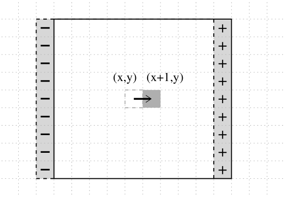
Figure 1: Basic principle of a rectangular-shaped 2D filter implementing 1D recursion

Gil and Werman took in [3] a similar approach processing the image in blocks of $(2n-1)^{2}$ pixels. They store all $(2n-1)^{2}$ pixels in a special search-tree based data structure that they call Implicit Offline Balanced Binary Search Tree (IOBBST). In fact, they use two nested IOBBST, i.e. each node of the main IOBBST contains a secondary IOBBST again. They do not rebuild this data structure as the running window moves inside the block but mark respective pixels as active or inactive. The algorithm is able to find $n^{2}$ medians in $O(n^{2}\log^{2}{n})$ time, further reducing the computational complexity of median calculation down to $O(\log^{2}{n})$ per pixel.

We are not aware of any implementation of Gil and Werman algorithm as well as no experimental evaluation was given in their article. However, the complexity of the algorithm flow suggests that the theoretical $O(\log^{2}{n})$ complexity translates to the real-world running time with a high (constant) factor.

The positive property of sorting-based approaches is that no assumptions about image data have to be made. A completely different approach is based on a histogram of pixel values. The median can be found by successive summing of histogram bins in increasing order until the sum reaches $n^{2}/2$. No difference between pixels falling into the same gray value range is made in this case. This can be beneficial for large $n$ and low number of histogram bins.

The Tibshirani’s Binmedian algorithm [7] belongs to such histogram-based algorithms, although it is not specifically intended for 2D image processing. It relies additionally on the Chebyshev’s inequality stating that the difference between the median $m$ and the mean $\mu$ is always at most one standard deviation: $|\mu-m|\leq\sigma$. The basic idea is to build a low resolution histogram of values in $[\mu-\sigma,\mu+\sigma]$ interval, i.e. map data values to bins inside this interval, find the bin which contains the median by successive summing of bins and then recur with finer histogram on values inside this bin until the required precision is reached. Relaxing precision requirements by not performing recursion on the median bin gives us the approximate version of Binmedian algorithm: Binapprox. It is accurate up to $1/B^{th}$ part of standard deviation, where $B$ is number of histogram bins.

The average case complexity of Binmedian algorithm is $O(n^{2})$ and the computational complexity of Binapprox was estimated as $O(n^{2})$ for the worst case. If applied to each image point independently they offer no significant advantage over the classic Quickselect. However, Binmedian and Binapprox algorithms can be used in update mode, reusing the histogram calculated at previous window position and only seldom resorting to full recomputation. An order of magnitude speedup was reported for this case [7].

All algorithms described above can work on data with arbitrary number of quantization steps or even floating point data. Further performance improvement can be made if fixed and a priori known gray value resolution is assumed. This is the case for most digital images and is especially advantageous for broadly used 256-values per channel images.

This approach is taken in the Huang et al. algorithm [5] where a 256-bin histogram is used for counting of gray values in a 2D moving window. The median calculation is performed in the same way as above by successive summing of individual histogram bins until the median condition is reached. This algorithm utilizes the overlap between two 2D windows at neighboring positions and updates the window histogram recursively. At each subsequent window position only values of the new pixel column are added to and values of the obsolete column are subtracted from the histogram calculated at previous position. This results in $O(n)$ computational complexity. Nevertheless the recursion is only one-dimensional and there is still room for improvements.

These have been done by Weiss in [8] who has improved Huang’s algorithm by using the distributive property of histograms. Weiss’s approach is to process several ($2n^{1/2}$, $4n^{2/3}$ up to $O(n)$) image rows at the same time and to maintain a set of partial histograms instead of using only one. These partial histograms reflect smaller image areas, than one single histogram would do, and thus, can be updated more efficiently. They are implicitly combined to a single histogram for final histogram-based median calculation. The same set of partial histograms is used for all rows which are processed simultaneously. Thus much of redundancy of Huang’s straightforward algorithm is avoided and average cost for histogram maintenance is lowered. Overall computational complexity becomes $O(\log{n})$.

Weiss’s algorithm can be also adapted to higher than 8-bit gray value resolutions via a technique called ordinal transform. It consists in sorting of all pixel values appearing in a given image and replacing them with their order-value. This allows more efficient histogram representation and associated arithmetic, saving space required for storage of histograms, but giving the algorithm $O(\log^{2}{n})$ complexity.

Perreault and Hébert [6] have chosen another way for improvement of Huang’s approach. They use separate histograms for each column of the moving window (which moves in horizontal direction). The column histograms are cached and can be efficiently updated in a recursive way. The window histogram is then created by summing of respective bins of column histograms. Since this is a linear operation, the window histogram can be recursively computed too. This requires subtraction of the column histogram which went out of scope of the running window and addition of the histogram for the column which was newly added to the window (Fig. 1). Both operations are constant time, i.e. the number of operations is independent of window size $n$. Albeit this number is significant, e.g. for 8-bit data it is 256 additions and 256 subtractions per resulting pixel. The calculation of median by summing of histogram bins also requires in average a constant time (127 additions and 128 comparisons in case of 8-bit data). Thus, neglecting initialization of column histograms for the first row and initial creation of the window histogram at the beginning of each row, which are $O(n)$ operations, the overall algorithm also becomes constant time. The high associated constant ought to be compensated by intensive usage of SIMD extensions (single instruction, multiple data) of modern vectorized CPUs. They also propose several heuristics for reducing of the high associated constant. The most powerful among them is to delay summation of column bins for the window histogram, till the respective bin is actually required for median calculation, i.e. to perform summation on-demand.

Another important refinement, applied by Perreault and Hébert (but first appeared in [1] by Alparone et al.), consists in usage of two-tier window histogram. The higher tier is called coarse level and consists of reduced number of bins (16 in this case), while the lower tier contains the usual full resolution histogram (256 bins). Such scheme allows to find the median faster by first scanning the low-resolution part and then continuing only in a limited range of the full-resolution histogram. Tibshirani’s successive binning algorithm [7] uses basically the same idea. It allows to reduce the average number of operations for finding median from 127 additions and 128 comparisons in case of 8-bit single-level histogram to roughly 16 additions and 16 comparisons using two-level histogram.

Note, the use of two-level histograms in Perreault and Hébert algorithm results in more important effect than just faster extraction of median. This procedure allows to reduce the number of potentially computationally intensive updates of bins in the window histogram because they are updated on-demand. Perreault and Hébert have analyzed computational complexity of their algorithm only for the version with full unconditional histogram update whereas the on-demand version is of practical interest. It was not done since it is difficult to track analytically. Our experimental results show that updates of window histograms are indeed the most time consuming part in Perreault and Hébert algorithm. This is an important observation and we fully develop an idea which addresses this problem in our algorithm.

III Hierarchical recursive running median

The main idea of the proposed algorithm is to optimize the calculation of various order statistics, and median among them, using a special data structure which we call interval-occurrences tree (IOT).

An interval of pixel values, defined by the lower and the upper bound, is associated with each node of the IOT. Each IOT node stores the number of occurrences of pixels which gray values belong to these intervals. An IOT is build in the following way (Fig. 2):

The top-most node has minimal possible pixel value as lower bound and maximal possible pixel value as higher bound. Number of occurrences is equal to the overall number of pixels in the region which is described by the IOT, i.e. all pixels are included.

Each node has exactly two children. They subdivide the interval of the parent node in two sub-intervals and store corresponding number of value-occurrences in each sub-interval.

Other nodes are defined recursively until the value interval associated with the node vanishes. For example, in case of integer data leaf nodes correspond to intervals of 1 gray value. Alternatively, the tree building can be stopped as soon as a required gray value precision is reached and thus floating point values can be processed too.

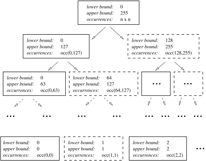
Figure 2: Interval-occurrences tree data structure. Each node has associated lower and upper bounds ($b_{lo}$ and $b_{up}$), which define an interval of pixel values, and stores the number of occurrences $occ(b_{lo},b_{up})$ of pixels with gray values inside this interval. Intervals and occurrences of child nodes sum to the interval and occurrences of their parent. Leaf nodes correspond to smallest possible (or smallest required) value intervals, e.g. 1 gray value in case of integer data.

Obviously, it is necessary to define how child-nodes divide the interval of their parent. The simplest rule would be to divide it in two equal-length parts. We will call such IOT a uniform interval-occurrences tree. Uniform IOT of height $d+1$ is necessary to represent integer data with effective bit-depth $d$ up to the precision of one gray value. We will address later how such an IOT can be created and stored in memory in an efficient way as well as how to fill and update it with pixel values.

Given a uniform IOT representation, any order statistic $k$ can be found by visiting at most $d$ nodes, requiring $d$ comparisons and in average $d/2$ additions.

Proof:

Consider the following algorithm for finding the smallest lower value interval with number of pixel occurrences equal or greater than $K=kn^{2}$, where $k$ is the requested percentile:

Get_order_statistic procedure:

Make topmost node the current one, set left_occurrences_accumulator to zero.

If number of occurrences in the left node (lower sub-interval) plus left_occurrences_accumulator is greater than the requested value $K$, then descend to the left sub-tree (Fig. 2), i.e. the sub-tree which further subdivides the left sub-interval. For this: make the left child node the current one. Otherwise: add number of occurrences in the left node (lower sub-interval) to the left_occurrences_accumulator and descend to the right sub-tree, making the right child node the current one.

If value interval corresponding to the current node is greater than the required precision, then repeat step III. Otherwise: return the lower interval bound corresponding to the current node.

The procedure above visits at most 8 nodes and makes at most 8 descends to sub-trees for 8-bit data and at most 16 nodes and descends for 16-bit data because these are the heights of the respective trees (excluding the topmost node). The returned value is equal, up to the required precision, to the value of $K$-th element of the list of individual pixel values sorted in ascending order and therefore it is the $k$-th order statistic by definition. ∎

The median filtering algorithm uses one IOT for the running window and separate IOTs of the same structure for each image column of size $n$ (assuming the running window moves in horizontal-first way). Same structure of two IOTs means that: (a) they are constructed for the same initial value interval, e.g. 0-255 gray values; (b) use the same rule for subdivision of the parent intervals into child intervals and (c) are built up to the same gray value resolution, e.g. 1 gray value. As the running window advances in horizontal direction its IOT is updated using column IOTs in a recursive way. That is: the number of value occurrences in a particular node of window IOT is decremented by the number of occurrences in the corresponding node of the column IOT which just went out of scope of the window and incremented by the value from the corresponding node in the column IOT which was just included in the window.

Node updates described above can be done for the entire window IOT. The computational complexity is proportional to the IOT size but independent of window size $n$, thus, it is an $O(1)$ operation with respect to $n$.

Instead of updating the entire window IOT, an on-demand update can be performed similarly as in [6] by updating only nodes actually required for median calculation at a given position. At most $d$ updates will be necessary since any order statistic can be found by visiting of $d$ nodes. Note that nodes on higher levels store occurrences corresponding to larger gray value intervals. The get_order_statistic procedure will with high probability visit the same nodes at the next window position. Such updates will require just one addition and one subtraction per visited node, i.e. are independent of $n$. We will call such updates elementary. Updates of nodes which were not visited since some window advances will require, however, execution of all delayed subtractions and additions, up to recalculation from scratch, requiring at most $n$ additions of occurrence counters in corresponding nodes of column IOTs.

As the running window advances to next image line, the column IOTs have to be updated too. This is also performed in a recursive way: new pixel values are added and obsolete values are subtracted from corresponding column IOTs, resulting in one added and one removed pixel per each column IOT. These are constant time operations too (exact description in next subsections).

One can see that the algorithm implements 2D recursion. The computational complexity of the version doing unconditional updates of the entire window IOT is independent of the window size $n$ for average as well as for the worst case. On-demand updates of the window IOT allow to further reduce the algorithm complexity for the average case.

Indeed, due to the hierarchical IOT design most updates are elementary (in our experiments with average data and $n\simeq 20..50$ about 95% of updates are elementary). Larger $n$ usually decreases the number of “costly” non-elementary updates because of smoother result. Upper complexity bound for a non-elementary update grows, however, with $n$.

Empirical data show that these two effects successfully compensate each other. Thus, the complexity of the algorithm doing on-demand update of the window IOT remains in average only approximately constant. The associated factor is, however, significantly lower than for the version which does unconditional updates of the entire window IOT and which constitute the upper complexity bound, strictly $O(1)$ but with a higher associated constant.

The proposed algorithm can be easily extended to N-dimensional case. Whereas the same is true for [6], the advantage in computational complexity of the developed algorithm will be higher and grow proportionally to data dimensionality.

III-A Implicit interval-occurrences tree and memory requirements

All IOTs in the above algorithm have the same structure. Therefore, lower and upper bounds of nodes’ sub-intervals can be stored only once in a single look-up table and need not to be repeated for each IOT.

A further significant improvement can be made by closer look at the get_order_statistic procedure. One can see that only the number of pixel occurrences stored in left nodes are used for order statistic calculation. This suggests that right nodes (shown on Fig. 2 with dashed line) need not to be stored in the IOT at all. Note that child nodes describe two value sub-intervals which build together the parent’s interval. In case the occurrences in the right sub-interval will be required at some later moment of time, they can be easily calculated by subtraction of the left sub-interval occurrences from the parent interval occurrences. Leaving out right nodes not only saves space, but, as it is shown in the next section, also saves computations during insertion and removal of pixel values in an IOT.

We call an IOT without right nodes implicit interval-occurrences tree. The number of nodes in an implicit IOT is calculated as sum of geometric series with common ratio of 2 and equals the size of a plain histogram for the same gray value range: $N=1+\sum_{i=1}^{d}{2^{i}/2}=1+\sum_{i=0}^{(d-1)}{2^{i}}=2^{d}$, where $1$ in the first part of this formula is for the top-most node, $i$ iterates from $1$ to $d$ because the tree has $d$ layers without the top-most node and the expression behind the sum sign is divided by 2 because only left nodes are stored explicitly.

There is no need for special memory allocations and storage of pointers to child nodes. The size of the (real part of) left sub-tree under each particular node can be found (for maximal gray value precision of 1) as $2^{d-i}-1$, where $i$ is depth of the node in a tree. Positioning the whole left sub-tree immediately after the parent node and applying this rule recursively, all nodes of any implicit uniform interval-occurrences tree can be stored in a vector and then accessed by indexing operations (Fig. 3). Such data organization also improves memory access pattern and cache utilization because data are accessed in sequential order with strictly increasing addresses (array indexes).

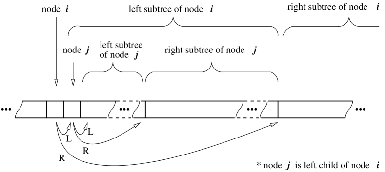
Figure 3: Storage of an implicit IOT as a vector. The whole left sub-tree is positioned immediately after the parent node. Right sub-tree (with missing root, because it is an implicit node) follows immediately after the left one. This is repeated recursively.

One can see that the use of implicit IOT reduces memory requirements in approximately two times, down to the same value as a plain single-layer histogram would require. This happens without any performance penalties. Instead a few operations during value additions/removals are even saved.

III-B Insertion and removal of pixel values in an IOT

Insertion (addition) of a value to an implicit uniform IOT can be done as follows (add_value procedure):

Make top-most node the current one. Increment by one occurrences stored here.

Make left child node the current one.

If the value to be inserted is lower than the upper bound of the current node, then increment by one occurrences stored here and descend into the left sub-tree, i.e. make left child node of the current node the new current one.
Otherwise: consider the implicit right node on the same level, which corresponds to the current (left) one (Fig. 2); incrementation of occurrences counter is not necessary since the node is an implicit one; just descend into the sub-tree growing from the implicit node, i.e. make left child node of the implicit node the current one.

If value interval size of the current node is greater than the predefined precision of the particular IOT, e.g. 1, then go to step III-B. Otherwise: finish.

Removal of a value is identical to the insertion with the only difference that the respective occurrences are decremented instead of being incremented. Both insertion and removal are constant time operations and require $d$ comparisons and in average $d/2$ additions per operation.

III-C Adaptive interval-occurrences tree

The number of additions and comparisons the algorithm makes directly depends on the tree height, which is 9 for a uniform IOT and 8-bit data and 17 for the 16-bit data. This height is constant for all values counted by a uniform interval-occurrences tree. It is, however, possible to build an interval-occurrences tree which has lower height for values which occur more frequently and allow a higher tree for seldom values, minimizing average height in this way. This is the same idea as used in entropy coding.

Let $T$ be a topology of interval-occurrences tree. Then the criterion for selection of the optimal $T$ can be formulated as

$$\min_{T}{\sum_{op\in OP}{p(op)h(op)}},$$

where $op$ is an operation for insertion/removal of a specific value or a calculation of a specific order statistic, $p(op)$ is relative frequency of occurrence of operation $op$, $h(op)$ is height of the IOT, i.e. number of nodes, visited to accomplish the request and the summation is performed over all operations $OP$ performed by filtering of an image. Note that $h(op)$ is defined by the tree topology $T$ and $T$ is the same for the window IOT as well as for the column IOTs. Thus, it has to be optimized for the value insertion/removal as well as for order statistic calculation at the same time.

Variable height can be implemented by allowing child sub-intervals to divide their parent’s interval into non-equal parts. We give it without proof that the optimization criterion is met if such sizes of sub-intervals are chosen that both children are visited equally frequent in course of algorithm execution.

The possibility of variable value intervals and variable height are properties which distinguish the IOT data structure from the conventional multi-tier histograms. That is why we give it a different name in general. The version utilizing the variable height is particularly called adaptive interval-occurrences tree.

Storage requirements of an adaptive implicit IOT remain the same as for the uniform one or the plain histogram. This follows from the following theorem: any data vector can be stored in a hierarchical structure requiring the same space as the original vector independently of the hierarchy’s topology.

Proof:

Consider a data vector $V$ of finite size $N$ (Fig. 4.a). An arbitrary element $V[k]$ can be made implicit and expressed via its sum with the following or the preceding element of $V$, e.g. $V[k]=S(k,k+1)-V[k+1]$, where $S(k,k+1)=\sum_{i=k}^{k+1}V[i]$. Thus, $S(k,k+1)$ can be stored instead of $V[k]$, see Fig. 4.b. Obviously, such representation still requires the same storage $N$. This can be repeated recursively for any $S(.,.)$ or another element of $V$, excluding those which are already used in some $S(.,.)$ (e.g. as in Fig. 4.c,d), until $S(1,N)$ is created. Then, one of many possible hierarchical representations is build. Storage requirements for any configuration and at any step are constantly $N$. ∎

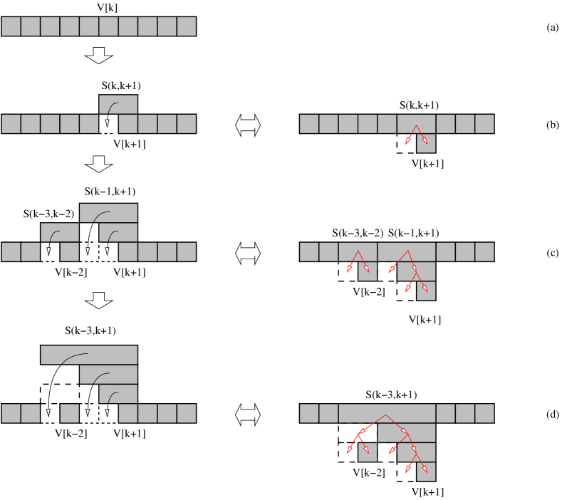
Figure 4: An example of hierarchical vector representation using implicit elements (shown dashed): (a) original data vector; (b)-(d) successive stages of conversion to a hierarchical representation. Obviously, storage space requirements remain constant and equal to the size of the original (plain) data vector independent of selection of elements which are grouped at next representation stage. Implicit elements can be always (recursively) recomputed from the higher element and its corresponding neighbor.

Topology of the adaptive IOT, i.e. lower and upper bounds of all subintervals, has to be stored only once for all IOTs used in the particular filter. Thus the added space requirements are negligibly small.

For the optimal IOT partitioning the frequencies have to be known at which particular nodes, i.e. the associated value intervals, are accessed. Value insertion and removal operations access intervals which correspond to values being inserted or removed. Thus, a conventional global histogram provides the necessary frequency information. On the other hand, the nodes accessed by the get_order_statistic procedure correspond to values of resulting median. Although they are generally not a priori known, a smoothed histogram of the median of a typical image is sufficient for this purpose. A running mean (its global histogram) can be also used as a first approximation, which is an $O(1)$ operation too. In video processing, the median distribution of the previous frame can be used.

Exactly one value insertion and one value removal is performed per one pixel of result image. Thus, we mix the source image global histogram and the global histogram of median estimation at 1:1 ratio. In case this mix vanishes for some value interval, it is just divided to equal parts, same as for the uniform IOT. Thus, without a priori knowledge about source data and filter result an adaptive IOT smoothly transforms into a uniform one.

III-D Variable precision

If the IOT-based median calculation does not descend down to leafs, which correspond to highest precision, but stops sooner, the result of median calculation is still meaningful. It just does not exhibit the maximal possible precision. The maximal error bound is also known: it is the width of the value interval corresponding to the last visited node. This allows to control the precision dynamically and independently for each image point. Important effect of the reduced precision on the algorithm performance is the avoidance of expensive non-elementary on-demand updates which occur for deeper nodes in the window IOT.

IV Experimental evaluation

The described algorithm for calculation of running median is implemented in C/C++. The source code is available under GPL from the algorithm web site (http://helios.dynalias.net/~alex/median). In course of experimental evaluation, the uniform IOT and the adaptive IOT versions of algorithm were compared to OpenCV implementation of [6] (http://opencv.willowgarage.com/). Special code snippets were included in implementation of both algorithms per conditional compilation for purpose of counting of additions and comparisons inherent to each algorithm. This way the data dependent number of operations performed in reality can be evaluated. Results of this evaluation for 8-bit data along with measurements of execution time (without this additional counting code) are given in Table I. Evaluation results for 16-bit data are given in Table II, although a comparison to Perreault and Hébert algorithm was not possible because of absent implementation of this algorithm for 16-bit data. Table II also includes results for reduced precision calculation on 16-bit data. Measurements of execution time are represented in number of CPU clock ticks utilized per output pixel. Evaluation is performed on Intel Core i7 M620 CPU (single core is used), code was compiled with gcc-4.4 without as well as with SIMD optimization.

The above comparison was done on various source images (Fig. 6) for one fixed size of the filter window. Fig. 5 shows algorithms’ performance for variable window size on example of one arbitrary image (“airfield”), demonstrating approximately constant computational complexity of both algorithms in the practically relevant window size range.

We purposely do not show here any filter results because they are the same irrespective of the applied algorithm.

We have also tested the Quickselect-based median filter on 16-bit data, as the most used one for non-8-bit data. It was slower than the proposed algorithm for window sizes larger than 4x4 pixels. Particularly, for window sizes 11x11 and 51x51 it was slower in approximately 3.9 and 43 times respectively.

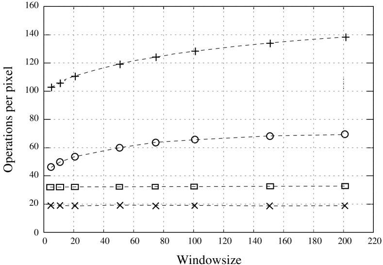
Figure 5: Average number of operations per output pixels made by the Perreault and Hébert [6] and the developed algorithm as function of filter size. 16 MPix “airfield” image (Fig. 6.a) is used. $+$ and $\times$ - additions and comparisons by Perreault, $\bigcirc$ and $\square$ - additions and comparisons by the uniform IOT version of the developed algorithm.

TABLE I: Operations breakdown (per pixel) and performance of Perreault and Hébert algorithm [6] and the uniform and adaptive versions of the developed algorithm for different source data. Filter window size $n$ is fixed to 51 pixels, because algorithm’ complexities are roughly independent of $n$. Additions and comparisons are listed separately. Runtime^∗ is number of CPU clock ticks utilized per pixel, Intel Core i7 M620 CPU (single core is used), compiled with gcc-4.4 with -00 -fno-tree-vectorize. Runtime^∗∗ is measured under the same conditions but compiling with -02 -ftree-vectorize. “Winner” is shown in bold font.

Algorithm	Maintenance of columns		Update of window		Median extraction		Overall per pixel		Runtime∗	Runtime∗∗
	add	cmp	add	cmp	add	cmp	add	cmp
Random uncorrelated normally distributed values, $\mu=128$, $3\sigma=128$, 4096 x 4096 image
Uniform  IOT	8.1	16.2	31.2	8.0	8.0	8.0	47.3	32.2	623	233
Adaptive IOT	8.4	36.0	16.1	4.0	4.6	7.9	29.1	47.9	717	333
Perreault & Hébert	4.4	0.0	86.6	1.0	21.2	19.2	112.2	20.2	1435	159
Real image with equalized histogram (classic “airfield” target up-scaled to 4096 x 4096)
Uniform  IOT	8.1	16.2	44.0	8.0	8.0	8.0	60.1	32.2	744	280
Adaptive IOT	8.1	33.0	44.7	8.2	8.8	16.4	61.6	57.6	1000	406
Perreault & Hébert	4.4	0.0	94.3	1.0	20.0	18.0	118.7	19.0	1543	170
Real image with compact histogram (“Venice at night”, 2532 x 3824)
Uniform  IOT	8.2	16.3	29.6	8.0	8.0	8.0	45.7	32.3	548	144
Adaptive IOT	4.0	14.2	14.7	3.2	4.2	6.4	22.8	23.9	368	126
Perreault & Hébert	4.4	0.0	78.9	1.0	7.3	5.3	90.5	6.3	1192	129
Worst case peak: synthetic diagonal sine pattern with 100 pix period
Uniform  IOT	8.1	16.2	100.3	8.0	8.0	8.0	116.4	32.2	1219	365
Adaptive IOT	9.2	34.6	100.8	8.4	9.4	16.9	119.4	60.0	1508	490
Perreault & Hébert	4.4	0.0	165.3	1.0	19.0	17.0	188.7	18.0	2495	223
Synthetic diagonal sine pattern with 25 pix period
Uniform  IOT	8.1	16.2	27.1	8.0	8.0	8.0	43.2	32.2	490	114
Adaptive IOT	7.8	28.5	9.9	3.0	3.9	6.0	21.7	37.5	482	168
Perreault & Hébert	4.4	0.0	77.2	1.0	12.9	10.9	94.5	11.9	1219	136

TABLE II: Operations breakdown and performance of uniform and adaptive versions of the developed algorithm on 16-bit data. Performance of uniform IOT for precision reduced down to 16 gray values included (“UIOT, err16”). Comparison to Perreault & Hébert is not possible because of missing implementation. Filter size is 51 and other conditions are the same as for Tab. I. Additionally, the performance in millions of pixels per second is given (single core of Intel Core i7 M620 CPU @ 2.67 GHz)

Algorithm	Maintenance of columns		Update of window		Median extraction		Overall per pixel		Runtime∗∗	Mp/s
	add	cmp	add	cmp	add	cmp	add	cmp
Random uncorrelated normally distributed gray values, $\mu=2^{15}$, $3\sigma=2^{15}$
Uniform  IOT	16.2	32.4	208.8	16.0	16.0	16.0	241.0	64.4	2025	1.32
UIOT, err16	16.2	32.4	80.4	12.0	12.0	12.0	108.6	56.4	1510	1.77
Adaptive IOT	16.9	68.2	194.8	11.7	12.3	23.4	224.0	103.3	3180	0.84
Real 16-bit image (industrial X-ray inspection of weldings)
Uniform  IOT	16.8	33.6	137.5	16.0	16.0	16.0	170.3	65.6	931	2.87
UIOT, err16	16.8	33.6	52.2	12.0	12.0	12.0	81.0	57.6	638	4.18
Adaptive IOT	13.5	54.6	129.4	12.9	13.5	25.8	156.5	93.3	1010	2.64
Worst case peak: synthetic diagonal sine pattern with 100 pix period
Uniform  IOT	16.2	32.4	477.5	16.0	16.0	16.0	509.7	64.4	4600	0.58
UIOT, err16	16.2	32.4	278.1	12.0	12.0	12.0	306.3	56.4	2935	0.91
Adaptive IOT	16.2	65.6	474.0	16.2	16.8	32.3	506.9	114.1	5040	0.53

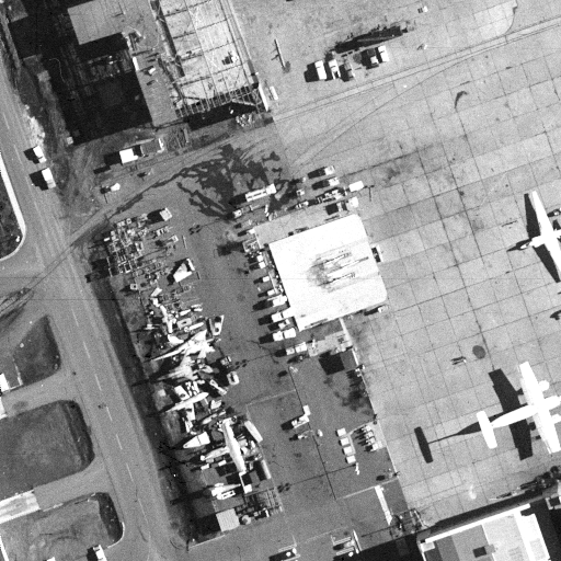
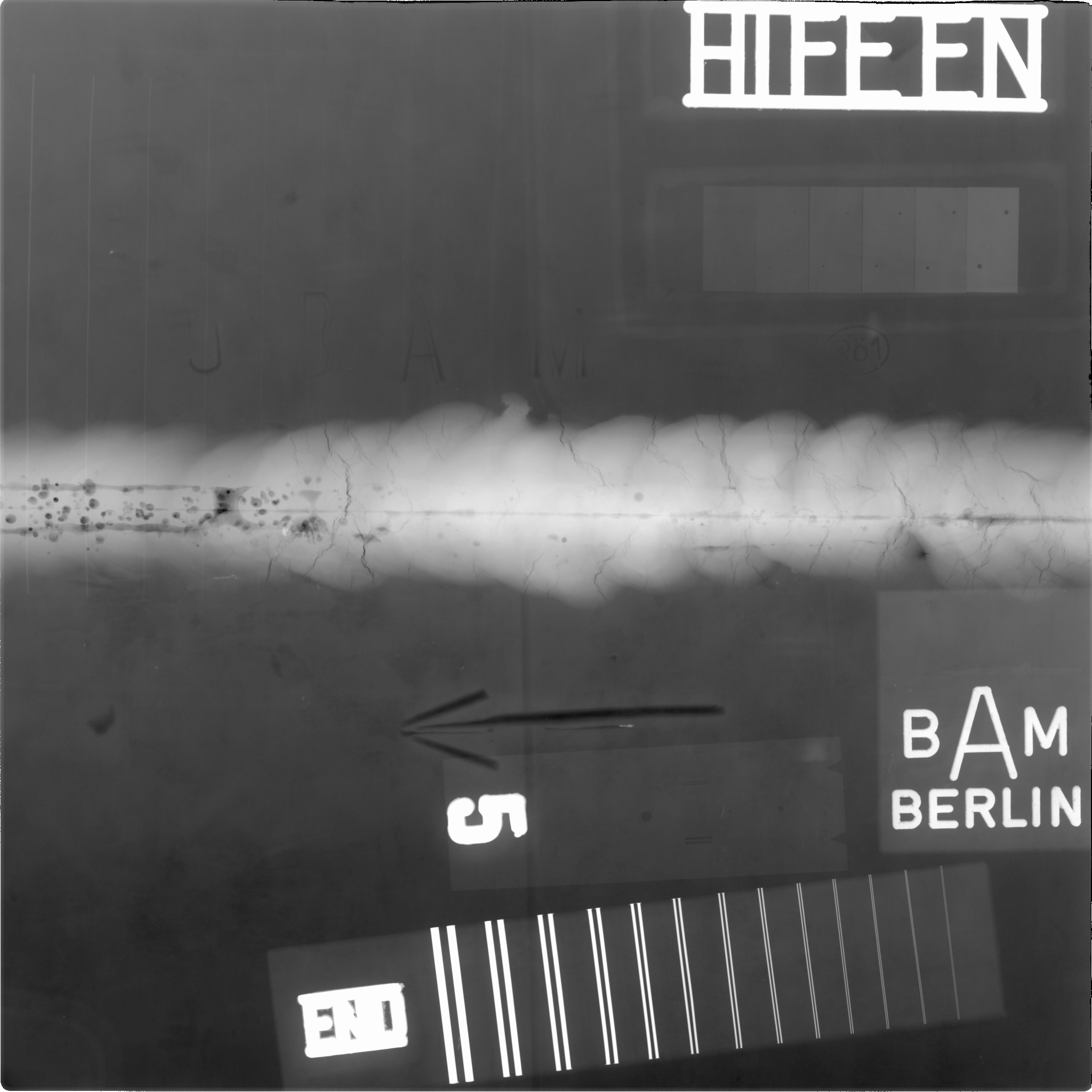
a)	b)	c)	d)

Figure 6: Test images used for evaluation: a) classic “airfield” image up-scaled to 4096 x 4096 with some uncorrelated uniformly distributed noise added to create high-frequency components (gray values fill whole 0..255 range and the histogram is fairly uniform); b) a low-key photograph (an 8-bit image with compact histogram); c) artificial worst case image similar to one used in [6]; d) X-ray inspection of a welding (a 16-bit image);

V Analysis

V-A Vectorized calculations

SIMD (single instruction, multiple data) is paralleling scheme implemented in hardware of many modern main stream CPUs. Using SIMD extensions several identical operations on vectors of data, e.g. several additions, subtractions or logical operations, can be performed in parallel in one execution step. Weiss [8] and Perreault and Hébert [6] propose to utilize SIMD instructions sets found on modern CPUs and accelerate running median calculation in this way. Their algorithms, based on plain histograms, benefit naturally of these possibilities.

The last two columns of Table I show how the execution time of Perreault and Hébert algorithm [6] can be improved thanks to SIMD and other hardware-specific optimizations. Although nearly twice as many additions have to be made by this algorithm, they can be executed in parallel, drastically reducing overall execution time. Whereas the developed algorithm requires in fact less operations as algorithm in [6], it cannot benefit from this hardware parallelism to the same great extend because of significantly higher number of branches (executed comparisons) in it.

Nevertheless, the developed algorithm makes less operations per pixel, offering therefore higher efficiency, and will be faster on CPUs without high internal parallelism.

V-B High precision data

The developed algorithm needs no modifications to be used on 16-bit images. A uniform IOT for 16-bit data has height of 16. It is twice as high as for 8-bit data, thus the first expectation for increase in number of operations is also a factor of two. However, as Table II shows, significantly more non-elementary updates of window IOT are required in practice. Despite the algorithm remains roughly $O(1)$, the increase in number of operations (for these data) is approximately a factor of 5. It is still an excellent result since, for example, in Weiss’s algorithm [8] the complexity would be squared.

We cannot perform experimental comparison to Perreault and Hébert algorithm for 16-bit data, because the corresponding implementation is not available. Instead of two-tier histogram they propose to use a three-tier or four-tier one for 16-bit data. We expect, however, that our approach will be superior because of fully optimized hierarchical data organization.

V-C Reduced precision output

Table II shows that performance is increased significantly if precision requirements are slightly relaxed. For this evaluation on 65536-gradation gray value data we allow an error of median estimation of $\simeq 0.02\%$ (i.e. 16 gray values). The error limit can be set for each individual pixel arbitrarily and independently, but for simplicity of evaluation we just set the same value for all pixels. For allowed error of 16 gray values the algorithm does not evaluate deepest 4 levels in the window IOT. This way many of non-elementary updates of nodes in window IOT are avoided (see “update of window” column of Table II).

V-D Data dependency and performance of adaptive IOT

Adaptive version of the developed algorithm requires one more comparison per node visit. It is because the tree has variable height and it must be always tested whether the node is a leaf. This is not necessary for uniform IOT where tree height is fixed and it is possible to determine in advance through how many layers the algorithm has to descend in order to reach leaf nodes. Thus the possibility of adaptation comes at added computational complexity costs (see operations breakdown in Tables I and II).

In order to be more efficient than the uniform version, the adaptive IOT must offer operation savings which compensate for these additional comparisons. The best case for this arises if gray value distribution of source image is highly correlated to gray value distribution of filtered image and if they show distinctive compact areas where most of gray values are located. If this is not the case, then the adaptive IOT version performs worse than its simpler uniform one. Thus, in our experiments the adaptive IOT version was able to show better performance only for images with compact histograms like the example in Fig. 6.b.

VI Conclusion and outlook

A new approximately constant time algorithm for calculation of running median and other order statistics is developed. The algorithm is based on a hierarchical data structure for storage of value occurrences in specific value intervals. The computational complexity of the algorithm is lowest among currently available algorithms. Experimental comparison to the single other constant time algorithm [6] confirms this. The competitive algorithm can, however, compensate its higher complexity by the extensive use of SIMD CPU extensions. Therefore it was not possible to show any practically relevant improvements of real-world execution time over it on 8-bit data if executed on a modern SIMD-enabled CPU.

Nevertheless, the new algorithm will be interesting for higher precision data and images with prevailing gray value ranges like HDR and X-ray imaging, low/high-key images, surveillance video, etc. as well as on platforms lacking hardware SIMD extensions, e.g. embedded systems, mobile devices, etc. Usual higher-level parallelizations are naturally possible too.

The developed algorithm needs no modifications to be used on 16-bit images. Straight-forward extension to 32-bit integer data becomes, however, impractical because of high memory requirements. Analogous, a general purpose extension for floating point data is not possible. The proposed by Weiss ordinal transform [8] can be used to address both problems, but will probably hamper performance. The usage of Chebyshev’s inequality as in [7] but in the IOT framework seams a better idea. This needs further investigations.

Alexander Alekseychuk has got his MS degree in electrical engineering from Lviv’s Institute of Technology (Lvivska Polytechnika) in 1994. Till 2000 he was with the Institute of Physics and Mechanics of the Ukrainian National Academy of Science. In 2000 he attended the German Federal Institute for Materials Research and Testing (BAM) where he dealt with algorithm and software development for image processing in application to digital industrial radiology. He has got his PhD degree for work in pattern recognition from the Technische Universität Dresden in 2006. Since 2010 he is with the Computer Vision and Remote Sensing Group at the Technische Universität Berlin. His former and current scientific interests are in the field of efficient algorithms, object detection on busy backgrounds and under low signal-to-noise ratios, texture-based segmentation and content-based image retrieval.

References

- [1] Luciano Alparone, Vito Cappellini, and Andrea Garzelli. A coarse-to-fine algorithm for fast median filtering of image data with a huge number of levels. Signal Process., 39:33–41, September 1994.
- [2] Robert W. Floyd and Ronald L. Rivest. Algorithm 489: the algorithm SELECT – for finding the i-th smallest of n elements [M1]. Communications of the ACM, 18:173, March 1975.
- [3] Joseph Gil and Michael Werman. Computing 2-d min, median, and max filters. IEEE Trans. Pattern Anal. Mach. Intell., pages 504–507, 1993.
- [4] C. A. R. Hoare. Algorithm 64, QUICKSORT. Communications of the ACM, 4(7):321–322, 1961.
- [5] T. Huang, G. Yang, and G. Tang. A fast two-dimensional median filtering algorithm. IEEE Trans. on Acoustics, Speech and Signal Processing, 27:13–18, Feb 1979.
- [6] Simon Perreault and Patrick Hébert. Median filtering in constant time. IEEE Transactions on Image Processing, 16(9):2389–2394, Sept. 2007.
- [7] Ryan J. Tibshirani. Fast computation of the median by successive binning. http://arxiv.org/abs/0806.3301v2, May 2009.
- [8] Ben Weiss. Fast median and bilateral filtering. In ACM SIGGRAPH 2006 Papers, SIGGRAPH ’06, pages 519–526, New York, NY, USA, 2006. ACM.