On the black hole limit of electrically counterpoised dust configurations

Abstract

By means of a simple scaling transformation any asymptotically flat Papapetrou-Majumdar solution of the Einstein-Maxwell equations corresponding to a localized regular distribution of electrically counterpoised dust can be reformulated as a one-parameter family of solutions admitting a black hole limit. In the limit, a characteristic separation of spacetimes occurs: From the exterior point of view, the extreme Reissner-Nordström metric outside the event horizon is formed. From the interior point of view, a regular, non-asymptotically flat (and in general non-spherically symmetric) spacetime with the extreme Reissner-Nordström near-horizon geometry at spatial infinity results.

1 Introduction

It is well-known that a parametric sequence of spherically symmetric perfect fluid bodies in equilibrium cannot come arbitrarily close to a black hole state: The radius, in Schwarzschild coordinates, has to be greater than $9/8$ times the corresponding Schwarzschild radius $2M$ [1]. In contrast, some rotating fluid bodies in equilibrium admit a continuous black hole limit. This was first demonstrated by Bardeen and Wagoner [2] in the limiting case of an infinitesimally thin disc of dust. A rigorous proof was provided by Neugebauer and Meinel [3] with the exact solution to the disc problem, see also [4, 5, 6]. In the limit, a “separation of spacetimes” occurs, leading to a non-asymptotically flat “inner world” and the extreme Kerr spacetime outside the horizon as the “outer world”. Numerically, such a black hole limit was found for fluid rings as well [7] and it was proved that it always leads to the extremal Kerr black hole [8]. Similar phenomena were observed for limiting solutions to the static Einstein-Yang-Mills-Higgs equations [9, 10]. However, the simplest examples can be constructed by means of solutions to the static Einstein-Maxwell equations belonging to the Papapetrou-Majumdar class [11, 12], sometimes called “Bonnor stars”. This was demonstrated in [13, 14, 15, 16, 17, 18]. The aim of the present paper is to treat the general black hole limit of such “electrically counterpoised dust” (ECD) configurations in much the same way as it was discussed for the rotating disc case in [2]. It is shown that a characteristic separation of spacetimes always occurs: From the exterior point of view, the extreme Reissner-Nordström metric outside the event horizon is formed. From the interior point of view, a regular, non-asymptotically flat spacetime with the extreme Reissner-Nordström near-horizon geometry at spatial infinity results. Whereas the outer world is spherically symmetric, the inner world does not need to show any spatial symmetry in general. As a concrete example, we consider the black hole limit of an ECD distribution of a triaxial ellipsoidal shape.

2 Configurations of electrically counterpoised dust

The Papapetrou-Majumdar class [11, 12] of static solutions to the Einstein-Maxwell equations can be described by the line element

$${\rm d}s^{2}=S^{2}({\rm d}x^{2}+{\rm d}y^{2}+{\rm d}z^{2})-S^{-2}{\rm d}t^{2}.$$ (1)

The corresponding energy-momentum tensor is given by

$$T_{ik}=\rho u_{i}u_{k}+T^{(\rm em)}_{ik},\quad u^{i}=\delta^{i}_{4}\,S,\quad\rho\geq 0,\quad S>0$$ (2)

with

$$T^{(\rm em)}_{ik}=\frac{1}{4\pi}(F_{ij}{F_{k}}^{j}-\frac{1}{4}F^{mn}F_{mn}g_{ik}),\quad F_{ik}=A_{k,i}-A_{i,k}$$ (3)

and

$$A_{i}=-\delta^{4}_{i}\,\phi,\quad\phi=-\epsilon(S^{-1}-1),\quad\epsilon=\pm 1.$$ (4)

The Einstein-Maxwell equations

$$R_{ik}-\frac{1}{2}R\,g_{ik}=8\pi T_{ik},{\quad F^{ik}}_{;k}=4\pi J^{i}$$ (5)

for the ECD case with

$$J^{i}=\sigma u^{i},\quad\sigma=\epsilon\rho$$ (6)

($\sigma$ being the charge density) are equivalent to

$$\Delta S\equiv\frac{\partial^{2}S}{\partial x^{2}}+\frac{\partial^{2}S}{\partial y^{2}}+\frac{\partial^{2}S}{\partial z^{2}}=-4\pi S^{3}\rho.$$ (7)

Expressing $S$ and $\rho$ by means of two new functions $V$ and $\mu$ according to

$$S=1-V,\quad\rho=\frac{\mu}{S^{3}}\,,$$ (8)

(7) can be rewritten as a Poisson equation:

$$\Delta V=4\pi\mu.$$ (9)

Asymptotically flat solutions, with a localized ECD distribution, can therefore be represented as a Poisson integral:

$$V=-\int\frac{\mu({\bf r^{\prime}})\,{\rm d}^{3}{\bf r^{\prime}}}{|{\bf r}-{\bf r^{\prime}}|},\quad{\bf r}=(x,y,z).$$ (10)

The asymptotic behaviour is given by

$$r\equiv|{\bf r}|\to\infty:\quad V\to-\frac{M}{r},\quad g_{44}=-S^{-2}\to-\left(1-\frac{2M}{r}\right)$$ (11)

with

$$M=\int\mu({\bf r})\,{\rm d}^{3}{\bf r}$$ (12)

being the gravitational mass, which is equal to the absolute value of the total charge $Q=\int\sigma S^{3}\,{\rm d}^{3}{\bf r}$.

3 The black hole limit

Any given solution belonging to an ECD distribution of finite extent can be characterized by a function $f({\bf r})$ vanishing outside some coordinate sphere of radius $r=R$ according to

$$\mu({\bf r})=f({\bf r})$$ (13)

with

$$f({\bf r})\equiv 0\quad\mbox{for}\quad r>R.$$ (14)

Alternatively, one can consider ECD distributions of infinite extent with a function $f({\bf r})$ decaying sufficiently rapidly as $r\to\infty$.

Now, let us consider a corresponding one-parameter family of solutions characterized by

$$\mu({\bf r})=\alpha^{3}f(\alpha{\bf r}),\quad\alpha>0.$$ (15)

For a function $f$ satisfying (14) this means

$$\mu({\bf r})\equiv 0\quad\mbox{for}\quad r>\frac{R}{\alpha}.$$ (16)

Note that $M$ does not depend on the parameter $\alpha$.

For sufficiently small values of $\alpha$ the Newtonian limit ($|V|\ll 1$) results. The black hole limit is obtained as

$$\alpha\to\infty.$$ (17)

In the coordinates used so far the ECD distribution shrinks to the point $r=0$ in the black hole limit. The metric for $r>0$ describes the “outer world”, while finite values of $\tilde{r}\equiv\alpha\,r$ reveal the “inner world” ($r=0$) in the limit $\alpha\to\infty$.

3.1 The exterior point of view

Formally, the limit $\alpha\to\infty$ leads to

$$\mu({\bf r})=M\delta({\bf r}).$$ (18)

Accordingly, we get

$$r>0:\quad V=-\frac{M}{r},\quad S=1+\frac{M}{r}$$ (19)

leading to

$${\rm d}s^{2}=\left(1+\frac{M}{r}\right)^{2}({\rm d}x^{2}+{\rm d}y^{2}+{\rm d}z^{2})-\left(1+\frac{M}{r}\right)^{-2}{\rm d}t^{2},$$ (20)

i.e. the metric of an extremal Reissner-Nordström black hole outside the event horizon, which is situated at $r=0$ in the isotropic coordinates used here.

3.2 The interior point of view

A completely different limit of the spacetime is obtained if the limit $\alpha\to\infty$ is performed after the coordinate transformation

$$\tilde{x}=\alpha x,\,\tilde{y}=\alpha y,\,\tilde{z}=\alpha z,\,\tilde{t}=\alpha^{-1}t$$ (21)

leading to the line element

$${\rm d}s^{2}={\tilde{S}}^{2}({\rm d}{\tilde{x}}^{2}+{\rm d}{\tilde{y}}^{2}+{\rm d}{\tilde{z}}^{2})-{\tilde{S}}^{-2}{\rm d}{\tilde{t}}^{2}$$ (22)

with $\tilde{S}=S/\alpha$. In the limit $\alpha\to\infty$ this means

$$\tilde{S}=\left.\alpha^{-1}S\right|_{\alpha\to\infty}=\left.\alpha^{-1}(1-V)\right|_{\alpha\to\infty}=\left.-\alpha^{-1}V\right|_{\alpha\to\infty}.$$ (23)

Together with (10), (15) and (21) we get

$$\tilde{S}=\int\frac{f(\tilde{\bf r}^{\prime})\,{\rm d}^{3}\tilde{\bf r}^{\prime}}{|\tilde{\bf r}-\tilde{\bf r}^{\prime}|},\quad\tilde{\bf r}=(\tilde{x},\tilde{y},\tilde{z}).$$ (24)

Note that all finite values of $\tilde{r}\equiv|\tilde{\bf r}|$ correspond to $r=0$ in the limit! The “inner world” described by (22), (24) is not asymptotically flat: Because of

$$\tilde{r}\to\infty:\quad\tilde{S}\to\frac{M}{\tilde{r}}$$ (25)

the line element, for large $\tilde{r}$, approaches asymptotically

$${\rm d}s^{2}=\frac{M^{2}}{\tilde{r}^{2}}({\rm d}{\tilde{x}}^{2}+{\rm d}{\tilde{y}}^{2}+{\rm d}{\tilde{z}}^{2})-\frac{\tilde{r}^{2}}{M^{2}}{\rm d}{\tilde{t}}^{2},$$ (26)

which is the extreme Reissner-Nordström “near-horizon geometry” [resulting from (20) for small $r$], also known as the Bertotti-Robinson metric or $AdS_{2}\times S^{2}$ spacetime. In fact, this solution to the Einstein-Maxwell equations already appeared in a classic paper by Levi-Civita that has recently been republished, see [19, 20]. Note that in the special case of finite and spherically symmetric ECD distributions the near-horizon geometry (26) holds exactly for all $\tilde{r}>R$.

The distribution of the mass-density $\rho$ as a function of $\tilde{\bf r}$ remains regular in the limit $\alpha\to\infty$ since

$$\rho=\frac{\mu}{S^{3}}=\frac{f(\tilde{\bf r})}{\tilde{S}^{3}}$$ (27)

for all $\alpha$. Remember that $f(\tilde{\bf r})$ vanishes for $\tilde{r}>R$ or decays sufficiently rapidly as $\tilde{r}\to\infty$.

3.3 An example

As a simple but nontrivial example we choose the function

$$f({\bf r})=\left\{\begin{array}[]{l}\mu_{0}\quad\mbox{for}\quad\frac{x^{2}}{a^{2}}+\frac{y^{2}}{b^{2}}+\frac{z^{2}}{c^{2}}\leq 1\\ 0\quad\mbox{elsewhere}\end{array}\right.$$ (28)

$$\mbox{with}\quad\mu_{0}={\rm constant}.$$ (29)

This represents a special ECD configuration with a triaxial ellipsoidal shape ($a$, $b$ and $c$ are the coordinate semiaxes). This example already shows the interesting effect of a non-spherically symmetric “inner world” mentioned in the introduction. For $a=b=c$ it reduces to the spherically symmetric model considered by Bonnor and Wickramasuriya [13]. The gravitational mass calculated according to (12) is

$$M=\frac{4\pi}{3}abc\,\mu_{0}.$$ (30)

Using the well-known formulae for the classical potential of a homogeneous ellipsoid, see, e.g., [21], the function $\tilde{S}$ given by (24) can be expressed as

$$\tilde{S}=\frac{3M}{4}\int\limits_{\lambda_{0}}^{\infty}\left[1-\frac{\tilde{x}^{2}}{a^{2}+\lambda}-\frac{\tilde{y}^{2}}{b^{2}+\lambda}-\frac{\tilde{z}^{2}}{c^{2}+\lambda}\right]\frac{{\rm d}\lambda}{\sqrt{(a^{2}+\lambda)(b^{2}+\lambda)(c^{2}+\lambda)}}\,,$$

where the lower integration limit $\lambda_{0}$ is defined according to

$$\lambda_{0}=0\quad\mbox{for}\quad\frac{\tilde{x}^{2}}{a^{2}}+\frac{\tilde{y}^{2}}{b^{2}}+\frac{\tilde{z}^{2}}{c^{2}}\leq 1\quad\mbox{and}$$ (31)

$$\frac{\tilde{x}^{2}}{a^{2}+\lambda_{0}}+\frac{\tilde{y}^{2}}{b^{2}+\lambda_{0}}+\frac{\tilde{z}^{2}}{c^{2}+\lambda_{0}}=1\quad\mbox{elsewhere}.$$

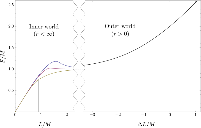
Figure 1: The metric function $F=rS=\tilde{r}\tilde{S}$ is plotted in the limit $\alpha\to\infty$. In the “inner world”, the variation of $F$ in the direction of the three principal axes of the ellipsoid is shown. $L$ is the proper distance from the center. The vertical lines indicate the intersection points of the axes with the surface of the ellipsoid. In the “outer world”, $\Delta L$ denotes the proper radial distance from the sphere $r=M$. The dashed line in the middle indicates the asymptotic value $F=M$ which holds for $\tilde{r}\to\infty$ ($L\to\infty$) as well as for $r\to 0$ ($\Delta L\to-\infty$), and corresponds to the “near-horizon geometry”.

Figure 1 combines the interior and the exterior point of view. We have chosen $b=0.8\,a$ and $c=0.5\,a$. The left part of the figure belonging to the “inner world” shows the variation of the function

$$F\equiv\tilde{r}\tilde{S}$$ (32)

with the proper distance

$$L=\int\limits_{0}^{\tilde{r}}\tilde{S}(\tilde{r}^{\prime})\,{\rm d}\tilde{r}^{\prime}$$ (33)

from the centre of the ellipsoid along the $\tilde{x}$-, $\tilde{y}$- and $\tilde{z}$-axis. According to (25), the asymptotic value of $F$ is given by

$$\tilde{r}\to\infty:\quad F\to M$$ (34)

in all directions. The right part of the figure belonging to the “outer world” shows the variation of the function

$$F\equiv rS$$ (35)

in any radial direction (note that the outer world is spherically symmetric). Here

$$\Delta L=\int\limits_{M}^{r}S(r^{\prime})\,{\rm d}r^{\prime}$$ (36)

denotes the proper radial distance from the arbitrarily chosen reference sphere $r=M$ (or $r_{\rm S}=2M$ in Schwarzschild coordinates). The proper radial distance of any place in the outer world ($r>0$) from $r=0$ (i.e. $r_{\rm S}=M$) is infinite. This is a characteristic feature of the extreme Reissner-Nordström metric (20). The limiting value of $F$ as $r\to 0$ is given by

$$r\to 0:\quad F\to M.$$ (37)

Thus the middle part of the figure with $F\equiv M$ (dashed line) belonging to the near-horizon geometry (26) represents the “connection” between the inner and the outer world. It should be stressed, however, that the inner world is a geodesically complete spacetime. These findings are in perfect analogy with the properties of the extreme relativistic limit of the rotating disc as discussed in [2], see figure 13 in that paper.

4 Discussion

The one-parameter families of solutions considered in this paper provide quasistatic routes from the Newtonian limit ($\alpha$ very small) up to the black hole limit ($\alpha\to\infty$) where the characteristic “separation of spacetimes” occurs. Configurations close to the limit ($\alpha$ very large but not infinite) are still characterized by a comprehensive, regular and asymptotically flat spacetime, which, for a distant exterior observer, is almost indistinguishable from the spacetime of an extremal Reissner-Nordström black hole outside the horizon. The term “quasi-black holes” used by Lemos and others, see [18], is a nice denotation for them. An interesting problem is the investigation of the stability of these quasi-black holes. It is to be expected that small perturbations, e.g. the infall of a small amount of (neutral) matter, will lead to a collapse and the formation of a genuine, slightly subextremal black hole. The investigation of the precise conditions for preventing the formation of naked singularities may lead to new insights concerning “cosmic censorship”. In addition, we mention that the extremal Reissner-Nordström black holes can be considered, in a sense, as classical models of point charges [22].

References

References

- [1] Buchdahl H A 1959 Phys. Rev. 116 1027
- [2] Bardeen J M and Wagoner R V 1971 Astrophys. J. 167 359
- [3] Neugebauer G and Meinel R 1995 Phys. Rev. Lett. 75 3046 (arXiv:gr-qc/0302060)
- [4] Meinel R 2002 Ann. Phys. (Leipzig) 11 509 (arXiv:gr-qc/0205127)
- [5] Meinel R, Ansorg M, Kleinwächter A, Neugebauer G and Petroff D 2008 Relativistic Figures of Equilibrium (Cambridge, UK: Cambridge University Press)
- [6] Kleinwächter A, Labranche H and Meinel R 2011 Gen. Relativ. Gravit. 43 1469 (arXiv:1007.3360 [gr-qc])
- [7] Ansorg M, Kleinwächter A and Meinel R 2003 Astrophys. J. 582 L87 (arXiv:gr-qc/0211040)
- [8] Meinel R 2006 Class. Quantum Grav. 23 1359 (arXiv:gr-qc/0506130)
- [9] Breitenlohner P, Forgács P and Maison D 1995 Nucl. Phys. B 442 126 (arXiv:gr-qc/9412039)
- [10] Lue A and Weinberg E J 2000 Phys. Rev. D 61 124003 (arXiv:hep-th/0001140)
- [11] Papapetrou A 1947 Proc. R. Irish Acad. 51 191
- [12] Majumdar S D 1947 Phys. Rev. 72 390
- [13] Bonnor W B and Wickramasuriya S B P 1975 Mon. Not. R. astr. Soc. 170 643
- [14] Bonnor W B 1998 Class. Quantum Grav. 15 351
- [15] Bonnor W B 1999 Class. Quantum Grav. 16 4125
- [16] Bonnor W B 2010 Gen. Relativ. Gravit. 42 1825
- [17] Lemos J P S and Weinberg E J 2004 Phys. Rev. D 69 104004 (arXiv:gr-qc/0311051)
- [18] Lemos J P S and Zaslavskii O B 2007 Phys. Rev. D 76 084030 (arXiv:0707.1094 [gr-qc])
- [19] MacCallum M A H 2011 Gen. Relativ. Gravit. 43 2297
- [20] Levi-Civita T 2011 Gen. Relativ. Gravit. 43 2307
- [21] Heymann O 1935 Astron. Nachr. 256 181
- [22] Arnowitt R, Deser S and Misner C W 1960 Phys. Rev. 120 321