Accuracy of the thin-lens approximation in strong lensing by smoothly truncated dark matter haloes

Abstract

The accuracy of mass estimates by gravitational lensing using the thin-lens approximation applied to Navarro-Frenk-White mass models with a soft truncation mechanism recently proposed by Baltz, Marshall and Oguri is studied. The gravitational lens scenario considered is the case of the inference of lens mass from the observation of Einstein rings (strong lensing). It is found that the mass error incurred by the simplifying assumption of thin lenses is below 0.5%. As a byproduct, the optimal tidal radius of the soft truncation mechanism is found to be at most 10 times the virial radius of the mass model.

1 Introduction

In recent years gravitational lensing has become the main tool in use to estimate the amount and distribution of matter of astrophysical systems of various kinds and sizes, from single compact objects to clusters of galaxies. Some very wide-ranging predictions rest on the accuracy of such mass estimates, most notably the value of the dark energy density and, with it, the time since the big bang. The predictive power of gravitational lensing as a tool to study individual deep objects also hinges heavily on the accuracy of the method. Consequently, any studies of the degree of accuracy of the method are naturally warranted. In this paper we describe a study that provides a quantitative measure of the degree of accuracy of the method in a particular context. Together with those of a previous study of ours [2008], these results are among the first quantitative estimates of the accuracy of the thin-lens approximation applied to gravitational lensing systems.

Our conceptualization of a gravitational lensing system is as follows: There is a physical “lens” that gravitationally disturbs the path of lightrays from a source to the observer. The theoretical framework for this situation would be a spacetime with a metric that solves the Einstein equations with a mass density source that describes the lens. The lightrays from the source to the observer would be null geodesics connecting both points. Even though the gravitational lensing event in itself (the null rays) is very amenable to a straightforward computational strategy, there is an intrinsic difficulty with this theoretical framework: the metric. This is determined by the mass density of the lens, also known as the density profile, and this, at this time, is still subject to modeling.

The conventional approach consists in making use of the thin-lens approximation to calculate the bending of lightrays. The conventional approach also makes use of the density profile assumed for the physical system. However, the quantities of interest in the conventional approach require a set of manipulations on the density profile that differ significantly from those needed in the theoretical framework. One significant difference resides in the fact that most quantities of interest in the conventional approach require the mass density integrated along the line of sight, a quantity referred to as the projected mass.

The conditions that a mass density must meet as a function in space in order to be useful for the conventional approach are much weaker than what is needed for the theoretical framework. The conventional approach admits density profiles that are not integrable over all space, namely, that have slow fall-off rates (slower than $r^{-3}$). Admittedly, such density profiles are unphysical in the sense that they do not represent the isolated systems that they intend to model. Nevertheless, they continue to be used because they are known to be a close approximation to the underlying physical system within a finite region centered on the lens. The question arises as to how to “terminate” such unphysical density profiles in the region where the approximation is not valid anymore (i.e., far from the lens).

The simplest way to terminate an unphysical density profile is by “hard” truncation, that is: by setting the profile discontinuously to zero beyond some radius. Arguably, this mechanism results in a density profile with questionable physical sense, especially because the truncation radius is largely arbitrary but also because discontinuous truncation introduces significant spurious magnification of images. However, the underlying system may be better approximated by such a drastically truncated density profile than by a non-integrable one, so the method is not devoid of merit.

Alternatively to hard truncations, various “soft” truncation mechanisms have been proposed, which normally consist of multiplicative factors that speed up the fall-off rate of the density profile in order to ensure a finite total mass.

In the present work we investigate how well the conventional approach to gravitational lensing estimates the mass of a lens, compared to the theoretical prediction. There are several subtleties associated with this seemingly straightforward task. To start with, the physical system itself (the actual density profile of a cluster in all space) is not known. What is known is a good representation of the density profile within a certain radius, referred to as the virial radius. Since the “true” density profile of the lens must be integrable over all space, we take the view that a profile with a finite total mass is the “true” system, and any other profile with a fall-off rate slower than $r^{-3}$ is an approximation to the true system, whose degree of accuracy must be quantified. In this view, a profile with an infinite total mass takes second seat to its truncated version, regardless of the truncation mechanism. This may sound contrary to prevailing practice, but is absolutely necessary to our goal because, in the theoretical framework, non-physical profiles result in inaccurate lightrays.

Taking a given truncated profile as the “true” physical system, there are thus two different approximations to quantify in relation to the “true” mass of the system as predicted by the theoretical approach: the error introduced by the thin-lens approximation and the further error introduced by the use of a profile that is integrable along the line of sight but which results in an infinite total mass. In this paper we refer to the latter as the error introduced by “removal of truncation”, for lack of a better phrase. Both errors are quantified in the present work within a given family of density profiles.

One can, and probably should, think of the truncation mechanism itself as an approximation: soft versus hard, for instance, or different kinds of soft truncation, all applied to the same model. In that case, it makes sense to quantify the error introduced by the truncation mechanism as a third source of inaccuracy in the mass estimates. We are able to provide an estimate of the truncation mechanism error by comparing mass predictions using soft and hard truncation schemes for the same class of density profiles.

The gravitational lens scenario considered is the case of the inference of lens mass from the observation of Einstein rings (strong lensing). The family of density profiles of interest is described in Section 2. The mass prediction by the conventional approach is discussed in Section 3. The calculation of the “true” mass as predicted by the theoretical framework is found in Section 4. The results of our study are found in Section 5 Section 6. We conclude in Section 7 with some remarks of interest that follow from our study.

2 Dark matter haloes

Numerical modeling of dark matter haloes predicts a density profile of the form [1997]

$$\frac{\rho(r)}{\rho_{\mbox{\scriptsize crit}}}=\frac{\delta_{c}}{\left(\frac{r}{r_{s}}\right)\left(1+\frac{r}{r_{s}}\right)^{2}},$$ (1)

hereafter referred to as the NFW model, where $\rho_{\mbox{\scriptsize crit}}$ is the critical density (given by $3H(z)^{2}/8\pi G$ in terms of the gravitational constant and Hubble’s constant at the lens redshift), $r_{s}$ is a scale radius defined as the peak of $r^{2}\rho(r)$, and $\delta_{c}$ is a characteristic density contrast. A “virial” radius is defined as the radius $r_{200}$ of the sphere with mean density equal to $200\rho_{\mbox{\scriptsize crit}}$, and is used to identify collapsed particle systems in numerical simulations. The ratio $r_{200}/r_{s}\equiv c$ is referred to as the halo’s concentration. By definition of the virial radius one has, as a consequence,

$$\delta_{c}=\frac{200}{3}\frac{c^{3}}{\log(1+c)-c/(1+c)}.$$ (2)

Falling off as $r^{-3}$, the NFW profile is not integrable over all space, which is interpreted as an indication that the model fails at large radius. Hence, a truncation mechanism is needed for long-range applications, such as gravitational lensing. Two truncation mechanisms for the NFW model have been used: hard truncation [2003, 2008] and smooth truncation [2009]. The hard-truncation mechanism consists of discontinuously terminating the model by assuming that the mass density is identically vanishing outside a given radius. In the lack of good knowledge pertaining to halo edges, the choice of termination radius is largely arbitrary. The common choice has been to terminate the NFW model at the virial radius.

The smooth truncation mechanism of Baltz et al. [2009] consists of multiplying the NFW profile by a factor that falls off at least like $r^{-2}$, being close to 1 within small values of $r$. This mechanism yields a sufficiently fast decay to ensure a finite total mass (at least $r^{-5}$), while preserving the original profile within a finite radius, within some accuracy. The smoothly truncated profile of Baltz et al. [2009] is

$$\rho_{n}(r)=\frac{\delta_{c}\rho_{\mbox{\scriptsize crit}}}{\left(\frac{r}{r_{s}}\right)\left(1+\frac{r}{r_{s}}\right)^{2}\left(1+\left(\frac{r}{r_{t}}\right)^{2}\right)^{n}}$$ (3)

where $n$ is a positive integer and $r_{t}$ is a parameter referred to as the tidal radius. For the purposes of the current investigation, we restrict attention to the case $n=1$, hereafter referred to as the truncated profile. For notational convenience we use $\rho_{0}$ for the NFW model, since clearly the expression (3) reduces to the NFW model (1) for $n=0$. If we use a rescaled coordinate $x\equiv r/r_{s}$, the virial radius would be located at $x=c$ and the tidal radius would be at $x=\tau\equiv r_{t}/r_{s}$. At any given radius $x$, the truncated profile $\rho_{1}$ differs from the NFW profile $\rho_{0}$ by

$$\frac{\rho_{1}(x)-\rho_{0}(x)}{\rho_{0}(x)}=-\frac{x^{2}}{x^{2}+\tau^{2}}.$$ (4)

As a consequence, one way to interpret the tidal radius is as the radius at which the profiles differ by 50%. At the virial radius the profiles differ by

$$\frac{\rho_{1}(c)-\rho_{0}(c)}{\rho_{0}(c)}=-\frac{1}{1+(\frac{\tau}{c})^{2}}.$$ (5)

Large values of the tidal radius $\tau$ relative to the virial radius thus ensure that the truncated profile remains sufficiently close to the NFW profile within the virial radius. For the profiles to differ by 10% or less at any point within the virial radius, the tidal radius needs to be chosen as $\tau=3c$ or larger. For this range of values of $\tau$, the virial mass (the mass contained within the virial radius) of the truncated profile differs from the virial mass of the NFW profile by less than 3%.

On the other hand, for large values of the tidal radius the truncated profile approaches the NFW profile, acquiring the undesirable features of the NFW model, such as a very large unrealistic total mass. The optimal value of $\tau$ would thus be the smallest possible value that yields the desired accuracy within the virial radius, which is somewhat arbitrary itself. Baltz et al. [2009] justify the choice of $\tau=2c$ on the basis that for this tidal radius the virial mass of the truncated profile differs from the NFW virial mass by only 6%. With this choice, however, the profiles themselves differ by up to 20% at the virial radius, a difference that may be considered significant. At any rate, the tidal radius should not be viewed as an independent parameter but should be considered a function of the concentration parameter. With this assumption, the models have two free parameters: the concentration parameter $c$ and the scale radius $r_{s}$.

3 Mass estimates by thin-lens gravitational lensing

We are interested in estimating the error in the prediction of the mass of a cluster by the observation of Einstein rings produced by the perfect alignment of a source of light behind a massive spherically symmetric deflector along the line of sight. In the usual manner [1992], the radius $s$ of the Einstein ring on the deflector’s plane (perpendicular to the line of sight) at a distance $D_{l}$ from us is the root of the lens equation:

$$1-\frac{M_{n}(s)}{\Sigma_{\mbox{\scriptsize cr}}\pi s^{2}}=0.$$ (6)

where $M_{n}(s)$ is the projected mass within a distance $s$ to the center of the lens:

$$M_{n}(s)\equiv 2\pi\int_{0}^{s}s^{\prime}ds^{\prime}\int_{-\infty}^{\infty}\rho_{n}\left(\sqrt{s^{\prime 2}+\ell^{2}}\right)d\ell.$$ (7)

The constant $\Sigma_{\mbox{\scriptsize cr}}$ is the characteristic surface mass density, given by

$$\Sigma_{\mbox{\scriptsize cr}}=\frac{c^{2}}{4\pi G}\frac{D_{s}}{D_{l}D_{ls}},$$ (8)

where $D_{s}$ is the distance to the source, $D_{ls}$ is the distance between the lens and the source, $G$ is the universal gravitational constant, and $c$ is the speed of light, not to be confused with the NFW concentration parameter.

For a given configuration of source and lens, different spherically symmetric models $\rho_{n}$ will predict different sizes of Einstein rings by virtue of the difference in their projected masses $M_{n}(s)$. In principle, given a known Einstein ring and known source and lens locations, equation (6) determines the concentration $c_{0}$ or $c_{1}$ of the NFW model or the truncated model, respectively, as functions of the scale radius $r_{s}$. Different concentrations $c_{0}$ and $c_{1}$ would lead to different predicted virial masses. In practice, we fix the value of the scale radius, the Einstein ring’s angle and the distances to the lens and the source, and determine the concentration by numerically solving equation (6) for $c_{n}$ to high accuracy using a standard bisection algorithm.

The value of the concentration parameter determines the virial mass of the model $M_{n}^{\mbox{\scriptsize 200}}$ by:

$$M_{n}^{\mbox{\scriptsize 200}}\equiv 4\pi\int_{0}^{c_{n}r_{s}}\!\!r^{2}\rho_{n}(r)dr$$ (9)

which, in the case of $n=0$, is equivalent to $M_{0}^{\mbox{\scriptsize 200}}\equiv c_{0}^{3}\pi\frac{800}{3}\rho_{\mbox{\scriptsize crit}}r_{s}^{3}$.

4 Mass estimates by numerical integration of the lightrays

The standard gravitational lensing formalism, leading to Eq.(6), assumes that the lightrays from the source to the observer are straight lines with sharp bending at the plane containing the deflector. The bending and all its consequences are obtained by “projecting” the mass density along the line of sight, namely, by integrating the mass density along the line of sight. This formalism is shadowed by a general relativistic formalism in which the lightrays from the source to the observer curve according to the geodesic equation of the metric of spacetime. The spacetime in this case is a lens with a weak gravitational field located on a expanding cosmological background. The lens is described by the truncated model $\rho_{1}$.

There is some leeway as to how to put together the metrics of an isolated lens and that of a Friedman-Robertson-Walker cosmology, in the sense that, to our knowledge, a rigorous and complete derivation of the Einstein equations valid for the particular case of an isolated lens on a cosmological background is still lacking. The Einstein equations matter because the motion of the spacetime affects the matter density, which affects the metric in turn. So long as the rigorous results remain outstanding, plausible (if unproven) descriptions of the behavior of the matter in the lens may need to be used. A widely accepted notion, supported by preliminary results, is that the matter distribution in a cluster of galaxies does not partake of the general expansion (namely, clusters do not expand internally). This can be modeled with a metric that approaches the standard cosmology at large distances from the lens, but which, in the vicinity of the lens itself, is indistinguishable from an isolated lens in flat space. Such a metric would be of the form

$$ds^{2}=(1+2\varphi(r,t))dt^{2}-a(t)^{2}(1-2\varphi(r,t))\{dr^{2}+r^{2}(d\theta^{2}+\sin^{2}\theta d\phi^{2})\}.$$ (10)

where $\varphi$ represents the non-expanding isolated lens centered at $r=0$. Wherever the function $\varphi$ is not negligibly small, the space part of the metric would be equivalent to that of an isolated lens on flat space if $\varphi(r,t)$ is the Newtonian potential of the lens in proper coordinates, namely $\varphi(r,t)=U(a(t)r)$ with $\nabla^{2}U=4\pi G\rho_{1}$. By requiring the solution of this equation to vanish at infinity and be finite at the origin, the Newtonian potential $U$ of the mass distribution $\rho_{1}$ is found to be

$$U(x)=\frac{Gm}{r_{s}}\frac{\tau^{2}}{(1+\tau^{2})^{2}}\Bigg{[}\arctan(x/\tau)\Big{(}\frac{1}{\tau}-\tau-2\frac{\tau}{x}\Big{)}+\ln\left(\frac{1+(x/\tau)^{2}}{(1+x)^{2}}\right)\Big{(}\frac{\tau^{2}-1}{2x}-1\Big{)}+\frac{\pi(\tau^{2}-1)}{2\tau}-2\ln\tau\Bigg{]}$$ (11)

with $x\equiv r/r_{s}$. Here $m\equiv 4\pi r_{s}^{3}\delta_{c}\rho_{\mbox{\scriptsize crit}}$.

The function $\varphi(r,t)$ is obtained by the substitution $r\rightarrow a(t)r$ in Eq. (11), and is, in principle, a time-varying function. However, the time variation is extremely slow in the conditions of observable lensing, where the source and observer are very far away from the lens. Since $\varphi$ is relevant only in the vicinity of the lens, one could substitute the time-varying $a(t)$ with a constant $a(t_{l})$ with $t_{l}$ being a representative time at which the lightray being considered reaches the vicinity of the lens. A posteriori, we find that the results of the numerical calculations that follow are not significantly affected by the choice of fixing the value of $a(t)$ to a constant, so we follow common practice and set

$$\varphi(r,t)=U(a(t_{l})r)$$ (12)

for use in the metric (10). This has the additional advantage that in these conditions the metric (10) is conformally static, as assumed in Schneider et al [1992], and thus the well known phenomena associated with lenses follow as per that text, including Eq. 6.

In the standard cosmology, the expansion parameter $a(t)$ is given by

$$a(t)=\left(\frac{\Omega_{m}}{\Omega_{\Lambda}}\right)^{1/3}\left\{\sinh\left(\frac{3H_{0}\sqrt{\Omega_{\Lambda}}t}{2}\right)\right\}^{2/3},$$ (13)

with $H_{0}=70$ km/s/Mpc, $\Omega_{m}=0.3$ and $\Omega_{\Lambda}=0.7=1-\Omega_{m}$.

Since the metric is spherically symmetric, we can restrict attention to the equatorial plane without loss of generality. The null geodesic equations are equivalent to the the Euler-Lagrange equations of the Lagrangian

$${\mathcal{L}}=(1+2\varphi)\dot{t}^{2}-a^{2}(t)(1-2\varphi)\{\dot{r}^{2}+r^{2}\dot{\phi}^{2}\}=0,$$ (14)

The Lagrangian is set to zero because the geodesics are null. The Euler-Lagrange equations are equivalent to five first-order ODEs, which we can write as

$$\dot{t} = v_{t}$$

$$\dot{r} = v_{r}$$

$$\dot{v}_{t} = -\frac{da}{dt}\frac{v_{t}^{2}}{a}-2(1-2\varphi)\frac{\partial\varphi}{\partial r}v_{t}v_{r}$$

$$\dot{v}_{r} = -\frac{2v_{t}v_{r}}{a}\frac{da}{dt}+4\frac{\varphi}{a^{2}}\frac{\partial\varphi}{\partial r}v_{t}^{2}$$

$$-\frac{2b^{2}}{a^{4}r^{2}}\frac{\partial\varphi}{\partial r}(1+6\varphi)+\frac{b^{2}}{a^{4}r^{3}}(1+4\varphi)$$

$$\dot{\phi} = -\frac{b}{a^{2}r^{2}}(1+2\varphi).$$ (15)

These equations are accurate to first order in $\varphi$. The parameter $b$ is a constant of integration and is related to the “observation angle” at the observer, or the angle between the lightray and the optical (radial) axis connecting the observer to the lens as explained in Kling & Frittelli [2008]:

$$\sin\theta_{obs}=\theta_{obs}=\frac{b}{r_{0}}(1+2\varphi_{0}),$$ (16)

where the potential $\varphi_{0}$, is evaluated at the observer position, $r_{0}$.

By integrating the equations of motion from a given point, for a specified set of parameters $(r_{s},c)$ describing the matter density, one finds a specific light ray passing through that point. Our scheme for a mass prediction is based on lightrays making Einstein rings, for which the source, lens and observer are collinear and are at known distances from each other. So the beginning and end point of the null geodesics being sought are known. In these conditions, for every observed Einstein ring $\theta_{obs}$, as per Eq. 16, there is an associated set of values of $(r_{s},c)$ that are consistent with the observed angle as well as the fixed configuration of lens, source and observer. As in the case of the prediction by the thin-lens gravitational lens formalism, in practice we fix $r_{s}$ and find $c$ using Newton’s method and a ray shooting technique. The ray shooting technique consists essentially of integrating rays for a given value of $c$ and seeing where they land with respect to the end point aimed at, either in front of it or behind it, subsequently adjusting $c$ accordingly, until the ray integrated lands sufficiently close to the target, within a specified accuracy. In practice, the integration is done from observer to source.

For the purposes of integrating the null geodesics, we re-scale the time and radial coordinates by the age of the universe. The equations of motion are integrated using an adaptive step-size Runge-Kutta-Fehlberg 4-5 method based on the implementation in [1995]. The numerical error is at least 500 times smaller than the difference between the result by null geodesic integration and the prediction by the thin-lens formalism.

The value of $c$ found by this method is considered to be the “true” value of the model and is used to predict the “true” virial mass of the model $M^{\mbox{\scriptsize 200}}$ by Eq. (9) with $n=1$, namely:

$$M^{\mbox{\scriptsize 200}}\equiv 4\pi\int_{0}^{cr_{s}}\!\!r^{2}\rho_{1}(r)dr.$$ (17)

5 Comparison of the thin-lens mass prediction relative to the null-geodesic prediction

For our first study we arbitrarily choose a series of five reasonable lensing systems with varying redshifts, and calculate the concentration parameters $(c,c_{1},c_{0})$ by the method of null-geodesics, thin-lens with truncation and thin-lens with no truncation, respectively. We do this for $\tau=2c$ and for $\tau=3c$ separately. In all cases, the scale radius is arbitrarily assumed to be $r_{s}=0.25$ Mpc. The results are shown in Tables 1 and 2.

In all cases, the concentration parameter $c_{1}$ is slightly higher than the true value $c$, whereas $c_{0}$ is closer to and generally lower than $c$. However, the reader should keep in mind that when the virial mass is used as the parameter for comparison, the relative values of $c_{0}$ and $c_{1}$ are not significant in themselves. The tables show for each case the errors in the virial masses of the truncated and non-truncated thin lens models relative to the true model (which is truncated with no assumption of thin lenses).

We can verify that, whether truncation is applied or not, the use of the thin-lens approximation overestimates the virial mass of the system, as the relative errors are negative in all cases.

The sizes of the two separate simplifying assumptions (thin lens and removal of truncation) are revealed to be very different. The error incurred by the sole simplifying assumption of thin lenses, displayed in the column headed by $1-M_{1}^{200}/M^{200}$, is generally between 0.3% and 0.7% for $\tau=2c$, and between 0.2% and 0.4% for $\tau=3c$.

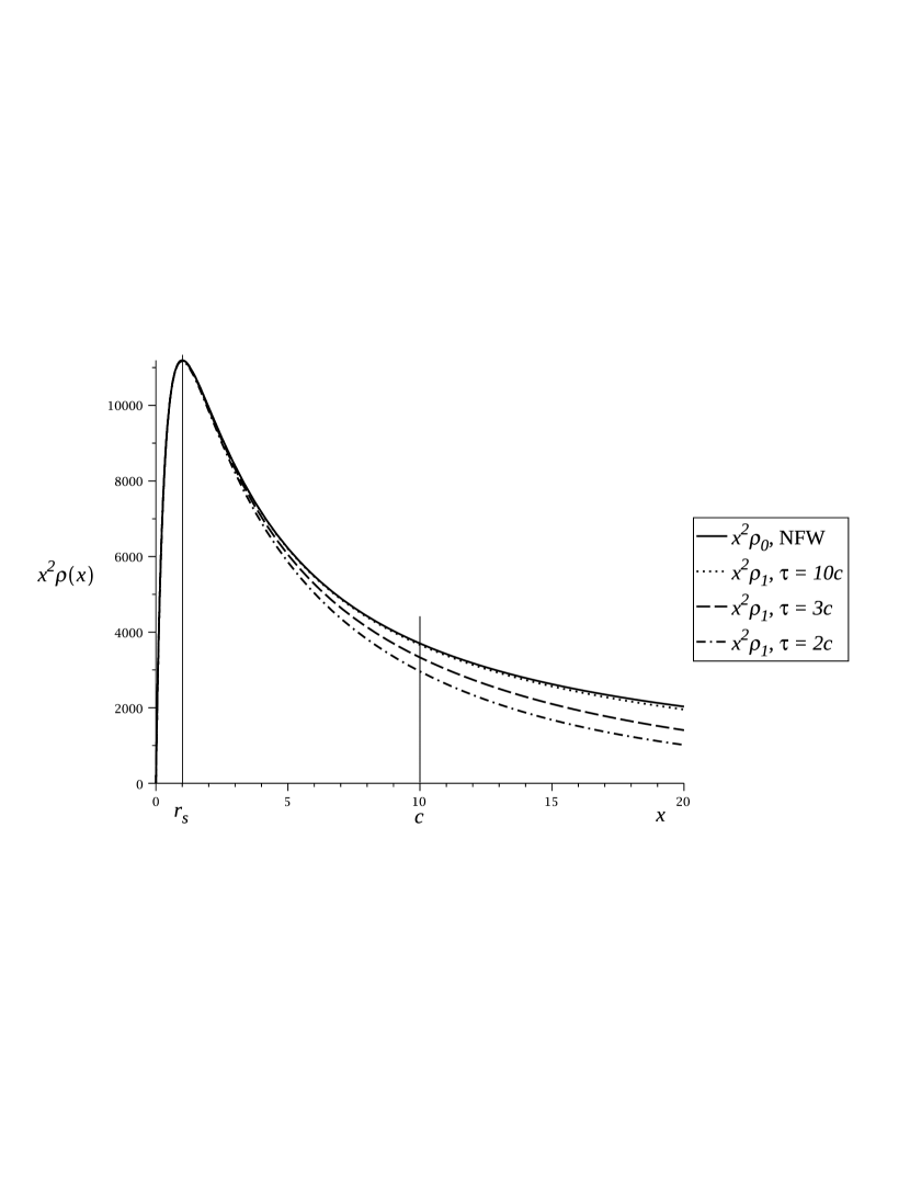
Figure 1: Density profiles as functions of the scaled distance $x\equiv r/r_{s}$. The solid line represents the standard NFW profile $x^{2}\rho_{0}(x)$, with a non-integrable fall-off. The other three lines represent the $n=1$ truncated profiles $x^{2}\rho_{1}(x)$ for three different values of the tidal parameter $\tau$ as multiples of the concentration $c$. All three truncated profiles have integrable fall-off rates. However, the larger the ratio $\tau/c$, the closer the truncated profile matches the NFW profile within the virial radius, represented by $c$ as a scaled distance.

By contrast, the error incurred by further removing the truncation in order to simplify the estimation of the mass is about 6% for $\tau=2c$ and 3% for $\tau=3c$. This is the dominant source of error in the virial mass. Keeping in mind that “truncation” in this model refers merely to a fast decay, this is not surprising, as different decay rates lead to significantly different profiles within the virial radius, as shown in Figure 1.

For our second study, we consider three observed systems with symmetrical arcs where one can use an Einstein ring analysis to determine parameters of the system with confidence. The systems are RXJ1347-1145, the brightest source in the ROSAT all sky survey [1998]; MS2137-23, a relatively structure-free, four-arc system [2003]; and cluster A of the high-redshift cluster RCS2319+00 [2008]. Table 5 gives the redshift and arc distribution details of these clusters.

For each one of these three systems, the Einstein rings are known. Modeling each system as a truncated $\rho_{1}$ density profile with $\tau=3c$ leads to two unknown parameters for each system: the value of the concentration parameter $c$ and the value of the scale radius $r_{s}$. The left panel of Figure 2 shows the contour plot in the $r_{s}-c$ plane for the Einstein rings of these three systems. For this plot, $r_{s}$ was varied arbitrarily and $c$ is the true concentration parameter determined using the null-geodesic integration formalism. In the right panel of Fig. 2, we show the error in the virial mass $1-M_{1}^{200}/M^{200}$. As the errors are negative, we verify that the thin-lens approximation overestimates the mass of each system. For reasonable values of $r_{s}$ and $c$, the errors are of the order of $0.5\%$.

Figure 3 shows the corresponding results for the case that the modeling is done with $\tau=2c$. One can verify that even though the concentration parameters do not differ significantly from the ones in the case of $\tau=3c$, the accuracy of the mass prediction is reduced by a factor of 2, as the maximum relative error in the mass is of the order of 10%.

6 Comparison of truncation mechanisms

As indicated in the introduction, one of the fundamental problems of gravitational lensing is the level of uncertainty in the underlying physical model of the lens irrespective of the approximation method used to make predictions. Here we address some of the consequences of this uncertainty by calculating the difference between the virial masses predicted exactly (with null geodesics) for two different models assumed to represent the same physical lens.

The two models differ in the truncation mechanism applied to an NFW lens: soft versus hard truncation. We use a density profile $\rho_{1}$ with $\tau=3c$ as a softly truncated NFW lens with $r_{s}=0.25$ Mpc. The hard truncation model is a density profile $\rho_{0}$ with $r_{s}=0.25$ Mpc within the virial radius, and zero outside of the virial radius. The hard truncation model is discussed extensively in our previous work [2008], where the gravitational potential needed for the integration of the null geodesics is found (Equation (34) in [2008]).

Table 4 shows the result of this study. The predicted virial masses for both models differ within $4\%$. This is an independent indication that the truncation mechanism itself is much more important than the simplifying assumption of thin lenses, and is the dominant source of error in mass estimates by gravitational lensing, by an order of magnitude. Perhaps counter-intuitively, the difference in profiles outside of the virial radius (as seen in Figure 1) is a significant source of inaccuracy in the prediction of virial mass by actual light paths traveled.

One puzzling result is that the hard truncation model consistently overestimates the mass with respect to the soft truncation model (as indicated by the negative values in the last column in Table 4). With both profiles being almost identical within the virial radius, one would expect that the soft truncation mechanism (just be virtue of having more total mass) would produce larger bending and would lead to a higher estimate for the virial mass.

7 Discussion

One of the main results obtained through our present study is that given a reasonable physical mass profile, such as $\rho_{1}$, the use of the thin-lens approximation as a simplifying assumption to predict the virial mass of the system leads to very small errors, which we found to be of order 0.5%. This can be interpreted as a validation of the use of the thin-lens approximation in the present context and, by extension, as an indication of the validity of the thin-lens approximation in generic physically reasonable systems.

A second result found is that, for this family of models, given a reasonable physical mass profile, such as $\rho_{1}$, removing the truncation as a further simplifying assumption (such as using the NFW) in addition to the thin-lens approximation leads to a significant loss of accuracy in the prediction of the virial mass of the system in the cases $\tau=2c$ and $\tau=3c$. The error introduced by removing the truncation is larger by a factor of at least 10 over the error introduced by the use of the thin-lens approximation.

For practitioners of the thin-lens approximation, one of the main concerns with the soft truncation mechanism studied here is the built-in $\tau$-dependent discrepancy in the mass profile. In effect, systems modeled with profiles $\rho_{1}$ with different values of $\tau/c$ can vary significantly. Because the truncation is effected by means of a modification of the decay rate, the profiles diverge over a significant range of distances. What is important, however, is that the $\tau-$profiles are reasonably close to the NFW profile $\rho_{0}$ within the virial radius. This is because the NFW profile is known to be accurate up to the virial radius, so any loss of accuracy within the virial radius is a disadvantage of the $\tau-$dependent model. Baltz et al [2009] propose that a discrepancy of about 20% in the mass profile between $\rho_{1}$ and $\rho_{0}$ is acceptable, as the penalty for working with a small tidal parameter $\tau=2c$.

However, larger values of the tidal parameter lead to better accuracy in the mass profile within the virial radius. We have argued and demonstrated that a slightly higher value $\tau=3c$ cuts the error in both the virial mass and density profile by half. Raising the value of $\tau$ relative to $c$ increases the accuracy of the profile, in principle arbitrarily. However, a profile $\rho_{1}$ for high $\tau$ can approach $\rho_{0}$ too accurately to be useful, if the predicted virial mass $M_{1}^{200}$ approaches $M_{0}^{200}$ more accurately than the limiting accuracy of the thin-lens approximation itself. In other words, since the thin-lens approximation itself carries a base accuracy of 0.5% in the virial mass prediction, there is no use in fine-tuning the density profile to lead to an accuracy better than 0.5% in the virial mass.

Our present study thus allows us to formulate a criterion for an optimal value of the tidal parameter $\tau$ relative to $c$: $\tau/c$ should be as large as possible but larger than required to achieve an accuracy of about $0.5\%$ in the virial mass $M_{1}^{200}$ relative to the NFW virial mass $M_{0}^{200}$. We can come up with a rough estimation by noticing that 20% accuracy in the profile leads to 6% accuracy in the virial mass, whereas 10% accuracy in the profile leads to 3% accuracy in the virial mass. The gross trend would indicate that 0.1% accuracy in the profile would achieve roughly 0.3% accuracy in the virial mass. By equation 5, a relative error of no less than 1% in the profile leads to a tidal radius no larger than $\tau\sim 10c$. A value of the order of $\tau=10c$ thus would guarantee that the NFW profile is modeled with $\rho_{1}$ within the virial radius to the limit of accuracy of the thin lens approximation, while ensuring that the model has a finite total mass.

This rough estimate is validated by Table 3 where the errors in the virial masses $M_{1}^{200}$ and $M_{0}^{200}$ relative to the true virial mass $M^{200}$ are shown in the last two columns. The column headed by $1-M_{1}^{200}/M^{200}$ represents the error incurred by the use of the thin lens approximation, and is generally of order of 0.2%. The last column, headed by $1-M_{0}^{200}/M^{200}$, represents the combined error of the thin lens approximation and lack of truncation, and is generally of order 0.4%. The difference between the values in both columns is the error introduced by the truncation mechanism alone, and is of order 0.2%, namely, comparable to the thin-lens approximation error, as anticipated. We claim that for thin-lens practitioners, using $\tau$ much greater than $10c$ would be inefficient, as it would lead to a truncation error smaller than the error inherently built into the thin-lens approximation itself.

Further validation of this claim is provided by Figure 4, where the relative virial mass errors $1-M_{1}^{200}/M^{200}$ and $1-M_{0}^{200}/M^{200}$ are calculated for values of $\tau=jc$ with $j=1,2,...15$, for the three observed systems of Table 5. One can see that in all three cases the thin-lens errors hover around 0.2%, whereas the combined truncation/thin-lens error drops dramatically from roughly 2% at $\tau=3c$ to less than 0.5% at $\tau=8c$, reaching within a factor of two of the thin-lens error at $\tau=10c$, indicating that the truncation error alone is of the same size as the thin-lens error at $\tau=10c$, as anticipated.

Other features to note from inspection of Tables 1, 2 and 3 are as follows. The larger the predicted mass, the more accurate the thin-lens prediction, with or without truncation. Nevertheless, the non-truncated prediction improves only marginally in accuracy, in contrast to the truncated prediction, which improves significantly.

8 acknowledgements

This material is based upon work supported by the National Science Foundation under Grant Nos. PHY-0244752 and PHY-0555218. We gratefully acknowledge the hospitality and support of the American Institute of Mathematics during the progress of the workshop “Gravitational Lensing in the Kerr Geometry,” AIM, Palo Alto, July 5-10, 2005.

$\tau=3c$
System	$\theta_{E}$	$r_{200}$ (Mpc)	$c$	$c_{1}$	$c_{0}$	$M^{\mbox{\scriptsize 200}}~{}(10^{15}M_{\odot})$	$1-M^{\mbox{\scriptsize 200}}_{1}/M^{\mbox{\scriptsize 200}}$	$1-M^{\mbox{\scriptsize 200}}_{0}/M^{\mbox{\scriptsize 200}}$
	10.0	2.05	8.201	8.210	8.204	1.14	-0.0033	-0.0289
$z_{l}=0.2$	17.5	2.29	9.153	9.161	9.154	1.60	-0.0028	-0.0274
	25.0	2.48	9.939	9.948	9.940	2.04	-0.0026	-0.0264
$z_{s}=0.4$	32.5	2.66	10.639	10.648	10.639	2.50	-0.0025	-0.0257
	40.0	2.82	11.282	11.291	11.281	2.98	-0.0025	-0.0251
	10.0	1.69	6.756	6.763	6.755	0.72	-0.0031	-0.0289
$z_{l}=0.3$	17.5	1.91	7.658	7.664	7.655	1.04	-0.0025	-0.0270
	25.0	2.10	8.415	8.421	8.410	1.38	-0.0022	-0.0257
$z_{s}=0.8$	32.5	2.27	9.093	9.100	9.087	1.74	-0.0021	-0.0248
	40.0	2.43	9.720	9.727	9.712	2.12	-0.0020	-0.0240
	5.0	1.34	5.376	5.384	5.377	0.36	-0.0045	-0.0319
$z_{l}=0.3$	9.0	1.49	5.972	5.979	5.971	0.50	-0.0035	-0.0297
	13.0	1.61	6.453	6.459	6.450	0.62	-0.0029	-0.0283
$z_{s}=1.5$	17.0	1.72	6.874	6.880	6.870	0.76	-0.0026	-0.0273
	21.0	1.81	7.258	7.264	7.253	0.88	-0.0024	-0.0265
	10.0	2.05	8.198	8.207	8.199	1.82	-0.0032	-0.0280
$z_{l}=0.6$	17.5	2.37	9.466	9.475	9.464	2.80	-0.0029	-0.0262
	25.0	2.64	10.546	10.556	10.544	3.86	-0.0029	-0.0251
$z_{s}=0.8$	32.5	2.88	11.521	11.533	11.518	5.04	-0.0030	-0.0243
	40.0	3.11	12.426	12.439	12.422	6.32	-0.0032	-0.0237
	5.0	1.30	5.205	5.214	5.205	0.74	-0.0049	-0.0313
$z_{l}=1.0$	9.0	1.48	5.933	5.941	5.930	1.10	-0.0038	-0.0286
	13.0	1.63	6.538	6.546	6.533	1.48	-0.0033	-0.0269
$z_{s}=1.5$	17.0	1.77	7.078	7.086	7.071	1.88	-0.0030	-0.0257
	21.0	1.89	7.576	7.584	7.567	2.30	-0.0029	-0.0247

Table 1: The concentration parameters and relative errors in the virial mass for a set of hypothetical lensing systems assuming that the true system has a density profile $\rho_{1}$ with a scale radius of $r_{s}=0.25$ Mpc and $\tau=3c$. We give the true $c$ value, and values obtained by thin lens approximations using a density profile $\rho_{1}$ ($c_{1}$) and an NFW profile $\rho_{0}$ ($c_{0}$). The virial radius quoted, $r_{\mbox{200}}$, is the one calculated using the true $c$ value. The true mass, $M^{\mbox{\scriptsize 200}}$ is given in units of $10^{15}$ solar masses.

$\tau=2c$
System	$\theta_{E}$	$r_{200}$ (Mpc)	$c$	$c_{1}$	$c_{0}$	$M^{\mbox{\scriptsize 200}}~{}(10^{15}M_{\odot})$	$1-M^{\mbox{\scriptsize 200}}_{1}/M^{\mbox{\scriptsize 200}}$	$1-M^{\mbox{\scriptsize 200}}_{0}/M^{\mbox{\scriptsize 200}}$
	10.0	2.05	8.202	8.216	8.204	1.12	-0.0049	-0.0611
$z_{l}=0.2$	17.5	2.29	9.156	9.168	9.154	1.54	-0.0040	-0.0579
	25.0	2.49	9.944	9.956	9.940	1.98	-0.0035	-0.0558
$z_{s}=0.4$	32.5	2.66	10.647	10.656	10.639	2.44	-0.0033	-0.0541
	40.0	2.82	11.289	11.300	11.281	2.90	-0.0031	-0.0528
	10.0	1.69	6.757	6.770	6.755	0.70	-0.0054	-0.0626
$z_{l}=0.3$	17.5	1.92	7.662	7.673	7.655	1.00	-0.0041	-0.0583
	25.0	2.11	8.421	8.431	8.410	1.34	-0.0035	-0.0555
$z_{s}=0.8$	32.5	2.28	9.102	9.111	9.087	1.70	-0.0031	-0.0533
	40.0	2.43	9.731	9.740	9.712	2.08	-0.0029	-0.0515
	5.0	1.34	5.374	5.389	5.377	0.34	-0.0087	-0.0696
$z_{l}=0.3$	9.0	1.49	5.973	5.986	5.971	0.48	-0.0066	-0.0649
	13.0	1.61	6.455	6.467	6.450	0.60	-0.0054	-0.0618
$z_{s}=1.5$	17.0	1.72	6.878	6.889	6.870	0.72	-0.0047	-0.0595
	21.0	1.82	7.264	7.274	7.253	0.86	-0.0042	-0.0577
	10.0	2.05	8.202	8.214	8.199	1.76	-0.0047	-0.0591
$z_{l}=0.6$	17.5	2.37	9.472	9.485	9.464	2.72	-0.0039	-0.0551
	25.0	2.64	10.556	10.568	10.544	3.76	-0.0036	-0.0525
$z_{s}=0.8$	32.5	2.88	11.533	11.547	11.518	4.92	-0.0035	-0.0505
	40.0	3.11	12.440	12.455	12.422	6.18	-0.0036	-0.0489
	5.0	1.30	5.206	5.221	5.205	0.72	-0.0091	-0.0680
$z_{l}=1.0$	9.0	1.48	5.937	5.950	5.930	1.06	-0.0067	-0.0622
	13.0	1.64	6.545	6.557	6.533	1.44	-0.0055	-0.0584
$z_{s}=1.5$	17.0	1.77	7.087	7.099	7.071	1.82	-0.0048	-0.0555
	21.0	1.90	7.587	7.598	7.567	2.24	-0.0044	-0.0532

Table 2: The concentration parameters and relative errors in the virial mass for a set of hypothetical lensing systems assuming that the true system has a density profile $\rho_{1}$ with a scale radius of $r_{s}=0.25$ Mpc and $\tau=2c$. We give the true $c$ value, and values obtained by thin lens approximations using a density profile $\rho_{1}$ ($c_{1}$) and an NFW profile $\rho_{0}$ ($c_{0}$). The virial radius quoted, $r_{\mbox{200}}$, is the one calculated using the true $c$ value. The true mass, $M^{\mbox{\scriptsize 200}}$ is given in units of $10^{15}$ solar masses.

$\tau=10c$
System	$\theta_{E}$	$r_{200}$ (Mpc)	$c$	$c_{1}$	$c_{0}$	$M^{\mbox{\scriptsize 200}}~{}(10^{15}M_{\odot})$	$1-M^{\mbox{\scriptsize 200}}_{1}/M^{\mbox{\scriptsize 200}}$	$1-M^{\mbox{\scriptsize 200}}_{0}/M^{\mbox{\scriptsize 200}}$
	10.0	2.05	8.199	8.205	8.204	1.18	-0.0022	-0.0045
$z_{l}=0.2$	17.5	2.29	9.149	9.155	9.154	1.64	-0.0020	-0.0042
	25.0	2.48	9.934	9.941	9.940	2.08	-0.0020	-0.0041
$z_{s}=0.4$	32.5	2.66	10.633	10.640	10.639	2.56	-0.0020	-0.0041
	40.0	2.82	11.274	11.282	11.281	3.06	-0.0021	-0.0041
	10.0	1.69	6.753	6.756	6.755	0.74	-0.0014	-0.0037
$z_{l}=0.3$	17.5	1.91	7.652	7.656	7.655	1.06	-0.0013	-0.0034
	25.0	2.10	8.408	8.411	8.410	1.42	-0.0013	-0.0034
$z_{s}=0.8$	32.5	2.27	9.084	9.089	9.087	1.78	-0.0014	-0.0033
	40.0	2.43	9.710	9.714	9.712	2.08	-0.0014	-0.0033
	5.0	1.34	5.375	5.378	5.377	0.36	-0.0015	-0.0038
$z_{l}=0.3$	9.0	1.49	5.970	5.972	5.971	0.50	-0.0012	-0.0035
	13.0	1.61	6.449	6.451	6.450	0.64	-0.0011	-0.0033
$z_{s}=1.5$	17.0	1.72	6.869	6.871	6.870	0.76	-0.0011	-0.0032
	21.0	1.81	7.252	7.254	7.253	0.90	-0.0011	-0.0031
	10.0	2.05	8.193	8.200	8.199	1.86	-0.0023	-0.0045
$z_{l}=0.6$	17.5	2.36	9.458	9.466	9.464	2.86	-0.0023	-0.0044
	25.0	2.63	10.536	10.545	10.543	3.94	-0.0025	-0.0044
$z_{s}=0.8$	32.5	2.88	11.510	11.520	11.518	5.14	-0.0027	-0.0046
	40.0	3.10	12.412	12.424	12.422	6.44	-0.0030	-0.0047
	5.0	1.30	5.203	5.206	5.205	0.76	-0.0020	-0.0042
$z_{l}=1.0$	9.0	1.48	5.928	5.932	5.930	1.12	-0.0018	-0.0039
	13.0	1.63	6.531	6.535	6.533	1.50	-0.0018	-0.0037
$z_{s}=1.5$	17.0	1.77	7.069	7.073	7.071	1.92	-0.0018	-0.0037
	21.0	1.89	7.565	7.569	7.567	2.34	-0.0019	-0.0037

Table 3: The concentration parameters and relative errors in the virial mass for a set of hypothetical lensing systems assuming that the true system has a density profile $\rho_{1}$ with a scale radius of $r_{s}=0.25$ Mpc and $\tau=10c$. We give the true $c$ value, and values obtained by thin lens approximations using a density profile $\rho_{1}$ ($c_{1}$) and an NFW profile $\rho_{0}$ ($c_{0}$). The virial radius quoted, $r_{\mbox{200}}$, is the noe calculated using the true $c$ value. The true mass, $M^{\mbox{\scriptsize 200}}$ is given in units of $10^{15}$ solar masses.

$r_{s}=0.25$ Mpc
System	$\theta_{E}$	$r_{200}^{\mbox{\scriptsize soft}}$ (Mpc)	$c_{\mbox{\scriptsize soft}}$	$c_{\mbox{\scriptsize hard}}$	$M^{\mbox{\scriptsize 200}}_{\mbox{\scriptsize soft}}~{}(10^{15}M_{\odot})$	$1-M^{\mbox{\scriptsize 200}}_{\mbox{\scriptsize hard}}/M^{\mbox{\scriptsize 200}}_{\mbox{\scriptsize soft}}$
	10.0	2.05	8.201	8.209	1.15	-0.0308
$z_{l}=0.2$	17.5	2.29	9.153	9.161	1.59	-0.0296
	25.0	2.48	9.939	9.947	2.04	-0.0287
$z_{s}=0.4$	32.5	2.66	10.639	10.647	2.51	-0.0281
	40.0	2.82	11.282	11.290	2.99	-0.0276
	10.0	1.69	6.756	6.766	0.71	-0.0340
$z_{l}=0.3$	17.5	1.91	7.658	7.668	1.04	-0.0324
	25.0	2.10	8.415	8.425	1.38	-0.0314
$z_{s}=0.8$	32.5	2.27	9.093	9.104	1.74	-0.0306
	40.0	2.43	9.720	9.731	2.13	-0.0300
	5.0	1.34	5.376	5.388	0.36	-0.0380
$z_{l}=0.3$	9.0	1.49	5.972	5.984	0.49	-0.0363
	13.0	1.61	6.453	6.464	0.62	-0.0351
$z_{s}=1.5$	17.0	1.72	6.874	6.886	0.75	-0.0343
	21.0	1.81	7.258	7.270	0.88	-0.0336
	10.0	2.05	8.198	8.207	1.81	-0.0313
$z_{l}=0.6$	17.5	2.37	9.466	9.475	2.79	-0.0298
	25.0	2.64	10.546	10.556	3.86	-0.0288
$z_{s}=0.8$	32.5	2.88	11.521	11.532	5.04	-0.0280
	40.0	3.11	12.426	12.437	6.33	-0.0274
	5.0	1.30	5.205	5.219	0.74	-0.0396
$z_{l}=1.0$	9.0	1.48	5.933	5.947	1.10	-0.0374
	13.0	1.63	6.538	6.552	1.47	-0.0361
$z_{s}=1.5$	17.0	1.77	7.078	7.093	1.87	-0.0351
	21.0	1.89	7.576	7.591	2.30	-0.0344

Table 4: The concentration parameters and relative error in the virial mass for a set of possible lensing systems modeled with soft truncation versus hard truncation. For soft truncation, the density profile is $\rho_{1}$ with $\tau=3c$. For hard truncation, the density profile is $\rho_{0}$ within the virial radius, and zero outside of the virial radius. The corresponding values of $c$ are both found by integration of the geodesic equations.

System	$z_{l}$	$z_{s}$	$\theta_{E}$ (arc sec)
RXJ1347-1145	0.45	0.80	35
MS2137+23	0.313	1.6	16
RCS2319+00A	0.9	3.86	12

Table 5: Three lensing systems analyzed in Figs. 2, 3 and 4. System RXJ1347-1145 is from Sahu et al. (1998), system MS2137+23 is from Gavazzi et al. (2003) and system RCS2319+00 is from Gilbank et al. (2008).

Figure 2: Contour in $(r_{s},c)$ space (left) and relative error between thin lens prediction and actual total mass (right) for the three lensing systems modeled as truncated distributions $\rho_{1}$ with $\tau=3c$. Circles correspond to the 35 arc sec arcs in RXJ1347-1145, triangles correspond to the 16 arc sec arcs in MS 2137-23, and squares correspond to the 12 arc sec arcs around cluster A of RCS 2319+00.

Figure 3: Contour in $(r_{s},c)$ space (left) and relative error between thin lens prediction and actual total mass (right) for three lensing systems modeled as as truncated distributions $\rho_{1}$ with $\tau=2c$. Circles correspond to the 35 arc sec arcs in RXJ1347-1145, triangles correspond to the 16 arc sec arcs in MS 2137-23, and squares correspond to the 12 arc sec arcs around cluster A of RCS 2319+00.

Figure 4: Relative error between thin lens prediction and actual total mass for three lensing systems for increasing values of $\tau$ as multiples of the concentration parameter ($\tau$ = jc). Filled symbols correspond to the truncated model $\rho_{1}$ and open symbols correspond to the non-truncated NFW model $\rho_{0}$.

References

- [2009] Baltz, E., Marshall, P. and Oguri, M., 2009, JCAP 0901:015
- [2003] Gavazzi, R., Fort, B., Mellier, Y., Pello, R., Dantel-Fort., M., 2003 Astron.Astrophysics, 403, 11
- [2008] Gilbank, D., Yee., H., Ellingson, E., Hicks, A.K., Gladders, M.D., Barrientos, L.F., Keeney, B. 2008, ApJ, 677, L89
- [2008] Kling, T.P., Frittelli, S., 2008, ApJ, 675, 115
- [1997] Navarro, J. F., Frenk, C. S., White, S. D.M., 1997, ApJ, 490, 493
- [1995] Press, W.H. et al., 1995, Numerical Recipes, Cambridge University Press
- [1998] Sahu, K. et al., 1998, ApJ, 492, L125
- [1992] Schneider, P., Ehlers, J. Falco, E.E., 1992 Gravitational Lenses, Springer-Verlag, Berlin, Heildelerg
- [2003] Takada, M., Jain, B., 2003, MNRAS, 340, 580