Non-uniqueness results for critical metrics of regularized determinants in four dimensions

Abstract.

The regularized determinant of the Paneitz operator arises in quantum gravity (see [Con94], IV.4.$\gamma$). An explicit formula for the relative determinant of two conformally related metrics was computed by Branson in [Bra96]. A similar formula holds for Cheeger’s half-torsion, which plays a role in self-dual field theory (see [Juh09]), and is defined in terms of regularized determinants of the Hodge laplacian on $p$-forms ($p<n/2$). In this article we show that the corresponding actions are unbounded (above and below) on any conformal four-manifold. We also show that the conformal class of the round sphere admits a second solution which is not given by the pull-back of the round metric by a conformal map, thus violating uniqueness up to gauge equivalence. These results differ from the properties of the determinant of the conformal Laplacian established in [CY95], [BCY92], and [Gur97].

We also study entire solutions of the Euler-Lagrange equation of $\log\det P$ and the half-torsion $\tau_{h}$ on $\mathbb{R}^{4}\setminus\{0\}$, and show the existence of two families of periodic solutions. One of these families includes Delaunay-type solutions.

1. Introduction

Let $(M^{n},g)$ be a closed Riemannian manifold. Let $\Delta=\Delta_{g}$ denote the Laplace-Beltrami operator, and label the eigenvalues of $(-\Delta_{g})$ by

$$0=\lambda_{0}<\lambda_{1}\leq\lambda_{2}\leq\dots$$

counting multiplicities. The spectral zeta function of $(M^{n},g)$ is

(1.1) $$\zeta(s)=\sum_{j=1}^{\infty}\lambda_{j}^{-s}.$$

By Weyl’s asymptotic law,

$$\lambda_{j}\sim j^{2/n},\ j\rightarrow\infty.$$

Consequently, (1.1) defines an analytic function for $\mbox{Re}(s)>n/2$.

Note that formally–that is, if we were to take the definition in (1.1) literally–then

(1.2) $$\zeta^{\prime}(0)=-\sum_{j=1}^{\infty}\log\lambda_{j}=-\log\det(-\Delta_{g}),$$

although of course the series (1.1) does not define an analytic function near $s=0$. However, one can meromorphically extend so that $\zeta$ becomes regular at $s=0$ (see [RS71]), and in view of (1.2) define the regularized determinant by

(1.3) $$\det(-\Delta_{g})=e^{-\zeta^{\prime}(0)}.$$

Since the determinant is obviously a global invariant, it is all the more remarkable that Polyakov was able to write a local formula (appearing as a partition function in string theory) for the ratio of the determinants for two conformal metrics on a closed surface (see [Pol81]). Suppose $\hat{g}=e^{2w}g$, then

(1.4) $$\log\frac{\det(-\Delta_{\hat{g}})}{\det(-\Delta_{g})}=-\frac{1}{12\pi}\int_{\Sigma}(|\nabla w|^{2}+2Kw)\ dA,$$

where $K=K_{g}$ is the Gauss curvature of $g$.

The formula (1.4) defines an action on the space of unit volume conformal metrics $[g]_{1}=\{e^{2w}g\ |\ Vol(e^{2w}g)=\int e^{2w}\ dA=1\}$. Critical points of this action are precisely those metrics of constant Gauss curvature; to see this one appeals to the Gauss curvature equation

(1.5) $$\Delta w+K_{\hat{g}}e^{2w}=K,$$

and computes a first variation of (1.4). In a series of papers [OPS88b], [OPS88a], Osgood-Phillips-Sarnak studied the existence of extremals for this functional, and the beautiful connection to various sharp Moser-Trudinger-Sobolev inequalities.

1.1. Four dimensions

In deriving (1.4) Polyakov exploited a crucial property of the Laplacian in two-dimensions, namely, its conformal covariance: if $\hat{g}=e^{2w}g$, then

$$\Delta_{\hat{g}}=e^{-2w}\Delta_{g}.$$

In general, we say that the metric-dependent differential operator $A=A_{g}$ is conformally covariant of bi-degree $(a,b)$ if $\hat{g}=e^{2w}g$ implies

(1.6) $$A_{\hat{g}}\psi=e^{-bw}A_{g}(e^{aw}\psi)$$

for each smooth section $\psi$ of some vector bundle $\mathbb{E}$. Examples of such operators include the conformal Laplacian

(1.7) $$L=-\Delta+\frac{(n-2)}{4(n-1)}R,$$

where $R$ is the scalar curvature, with $a=\frac{n-2}{2}$ and $b=\frac{n+2}{2}$, and the four-dimensional Paneitz operator

(1.8) $$P=(-\Delta)^{2}+\delta\left(\frac{2}{3}Rg-2Ric\right)\circ\nabla,$$

with $a=0$ and $b=4$. Indeed, the Paneitz operator is from many points of view the natural generalization of the Laplace-Beltrami operator to four-manifolds, and in analogy to the Gauss curvature equation we have the prescribed $Q$-curvature equation

(1.9) $$Pw+2Q=2Q_{\hat{g}}e^{4w},$$

where $Q$ is the $Q$-curvature:

(1.10) $$Q=\frac{1}{12}(-\Delta R+R^{2}-3|Ric|^{2}).$$

In [BO91], Branson-$\O$rsted were able to generalize Polyakov’s technique to conformally covariant operators $A$ defined on a four-manifold $M^{4}$. The resulting formula, while somewhat complicated, is geometrically quite natural. The first thing to note is that it is always a linear combination of three universal terms appearing in the determinant formula, with different linear combinations depending on the choice of operator $A$. Therefore, the formula is typically expressed as

(1.11) $$F_{A}[w]=\log\frac{\det A_{\hat{g}}}{\det A_{g}}=\gamma_{1}(A)I[w]+\gamma_{2}(A)II[w]+\gamma_{3}(A)III[w],$$

where $(\gamma_{1},\gamma_{2},\gamma_{3})$ is a triple of real numbers, and $I,II,III$ are the three sub-functionals. For example, if $A=L$, the conformal Laplacian, then

(1.12) $$\gamma_{1}(L)=1,\qquad\gamma_{2}(L)=-4,\qquad\gamma_{3}(L)=-2/3.$$

In general, if $A$ has a non-trivial kernel, then one needs to modify the definition of the zeta function (since $0$ is an eigenvalue); this results in some additional terms in the formula for $F_{A}$, see [BO91].

Before giving the precise formulas for these functionals, it may shed some light if we first describe their geometric content:

$$\hat{g}=e^{2w}g\ \mbox{is a critical point of }I\ \Longleftrightarrow|W_{\hat{g}}|^{2}=const.,$$

$$\hat{g}=e^{2w}g\ \mbox{is a critical point of }II\ \Longleftrightarrow Q_{\hat{g}}=const.,$$

$$\hat{g}=e^{2w}g\ \mbox{is a critical point of }III\ \Longleftrightarrow\Delta_{\hat{g}}R_{\hat{g}}=0,$$

where $W$ is the Weyl curvature tensor. Thus, each functional corresponds to a natural curvature condition in four dimensions. The functionals $II$ and $III$ are of particular interest as they correspond to, respectively, the constant $Q$-curvature problem and the Yamabe problem.

1.2. The formulas

The precise formulas for $I$, $II$, and $III$ are

(1.13) $$I[w]=4\int w|W|^{2}\ dv-\big{(}\int|W|^{2}\ dv\big{)}\log\fint e^{4w}\ dv,$$

(1.14) $$II[w]=\int wPw\ dv-\big{(}\int Q\ dv\big{)}\log\fint e^{4(w-\overline{w})}\ dv,$$

(1.15) $$III[w]=12\int(\Delta w+|\nabla w|^{2})^{2}\ dv-4\int(w\Delta R+R|\nabla w|^{2})\ dv.$$

In order to write down the Euler-Lagrange equation for $F_{A}$, we define the following conformal invariant:

(1.16) $$\kappa_{A}=-\gamma_{1}\int|W|^{2}\ dv-\gamma_{2}\int Q\ dv.$$

Then the E-L equation is

(1.17) $$\begin{split}\mu e^{4w}&=(\frac{1}{2}\gamma_{2}+6\gamma_{3})\Delta^{2}w+6\gamma_{3}\Delta|\nabla w|^{2}-12\gamma_{3}\nabla^{i}\big{[}(\Delta w+|\nabla w|^{2})\nabla_{i}w\big{]}\\ &\hskip 18.06749pt+\gamma_{2}R_{ij}\nabla_{i}\nabla_{j}w+(2\gamma_{3}-\frac{1}{3}\gamma_{2})R\Delta w+(2\gamma_{3}+\frac{1}{6}\gamma_{2})\langle\nabla R,\nabla w\rangle\\ &\hskip 21.68121pt+(\gamma_{1}|W|^{2}+\gamma_{2}Q-\gamma_{3}\Delta R),\end{split}$$

where

(1.18) $$\mu=-\frac{\kappa_{A}}{\int e^{4w}}.$$

Note the equations are in general fourth order, unless $\frac{1}{2}\gamma_{2}+6\gamma_{3}=0$. In this case the equation is second order but fully nonlinear; it is precisely the $\sigma_{2}$-curvature condition (see [Via00]).

Geometrically, (1.17) means the following: denote the $U$-curvature of $g$

(1.19) $$U=U(g)=\gamma_{1}|W|^{2}+\gamma_{2}Q-\gamma_{3}\Delta R.$$

If $w$ satisfies (1.17), then the conformal metric $g_{A}=e^{2w}g$ satisfies

(1.20) $$U(g_{A})\equiv\mu.$$

1.3. Some general existence results

The first existence results for extremals of the functional determinant in four dimensions were proven by Chang-Yang [CY95].

Theorem 1.1.

(Chang-Yang, [CY95]) Assume:

$(i)$ $\gamma_{2}<0$ and $\gamma_{3}<0$,

$(ii)$ $\kappa_{A}<(-\gamma_{2})8\pi^{2}$.

Then $\sup_{w\in W^{2,2}}F_{A}[w]$ is attained by some $w\in W^{2,2}$.

For example, taking $A=L$ the conformal Laplacian, then an extremal exists for $F_{L}$ provided

(1.21) $$\kappa_{L}(M^{4},g)=-\int|W|^{2}\ dv+4\int Q\ dV<32\pi^{2}.$$

This condition is related to the best constant in the Moser-Trudinger inequality of Adams [Ada88], and eliminates the possibility of bubbling (note for the round sphere, $\kappa_{L}=32\pi^{2}$). Regularity of extremals was proved by the first author in joint work with Chang-Yang [CGY99]; later Uhlenbeck-Viaclovsky proved a more general regularity result for any critical point of (1.17) (see [UV00]).

The first author established that the condition (1.21) is always satisfied by a $4$-manifold of non-negative scalar curvature, unless it is conformally equivalent to the round sphere [Gur99]. In this case, Branson-Chang-Yang proved that the round metric, and its orbit under the conformal group, maximizes $F_{L}$ [BCY92]. Later, the first author proved that the round metric (modulo the conformal group) is the unique critical point [Gur97]. Thus the existence theory for $F_{L}=\log\det L$, at least for $4$-manifolds of positive scalar curvature, is complete, and we have uniqueness (modulo the conformal group) on the sphere.

In general situations not much is known about existence of critical points. In [DM08] the functional $II$ is studied in generic situations, and saddle points solutions are found using a global variational scheme.

1.4. Determinant of the Paneitz operator and Cheeger’s half-torsion

In this paper we are interested in regularized determinants for which condition $(i)$ of Theorem 1.1 fails; i.e., the coefficients $\gamma_{2}$ and $\gamma_{3}$ have different signs. The corresponding functionals are therefore non-convex combinations of terms with different homogeneities, and their variational properties quite difficult to analyze. This arises in two cases of interest in mathematical physics: the determinant of the Paneitz operator, and Cheeger’s half-torsion.

In his book Noncommutative Geometry, Alain Connes devoted a section to the discussion of the determinant of the Paneitz operator (see [Con94], Chapt. IV.4.$\gamma$), ending with the remark that ”…the gravity theory induced from the above scalar field theory in dimension $4$ should be of great interest…” In [Bra96], Branson calculated the coefficients of $F_{P}$ and found $(\gamma_{1},\gamma_{2},\gamma_{3})=(-1/4,-14,8/3)$.

For even-dimensional manifolds the half-torsion is defined by

(1.22) $$\tau_{h}=\frac{\displaystyle(\det(-\Delta_{0}))^{n}(\det(-\Delta_{2}))^{n-4}\dots}{\displaystyle(\det(-\Delta_{1}))^{n-2}(\det(-\Delta_{3}))^{n-6}\cdots},$$

where $\Delta_{p}$ denotes the Hodge laplacian on $p$-forms. Notice that this only involves $p$ for $p<n/2$; in particular in four dimensions we have

(1.23) $$\tau_{h}=\frac{\displaystyle(\det(-\Delta_{0})^{4}}{\displaystyle(\det(-\Delta_{1}))^{2}}.$$

The half-torsion plays a role in self-dual field theory, for which the dimensions of physical interest are $n=4\ell+2$. Witten’s novel approach to studying self-dual field theory involved using Chern-Simons theory in $4\ell+3$-dimensions (see [Wit97]). Cheeger’s half-torsion appears when computing the metric dependence of the partition function, similar to Polyakov’s formula ([BM], [Mon]). Note that although the Hodge laplacian in general does does not satisfy (1.6), the ratio in (1.22) has the requisite conformal properties for deriving a Polyakov-type formula (see [Juh09], Section 6.15). The coefficients for the corresponding functional are $(\gamma_{1},\gamma_{2},\gamma_{3})=(-13,-248,116/3)$.

In this paper we consider these functionals in the case of the round $4$-sphere. For the determinant of the Paneitz operator we have

(1.24) $$\begin{split}F_{P}[w]&=\int\Big{[}18(\Delta w)^{2}+64|\nabla w|^{2}\Delta w+32|\nabla w|^{4}-60|\nabla w|^{2}\Big{]}\ dv\\ &\hskip 36.135pt+112\pi^{2}\log\Big{(}\fint e^{4(w-\overline{w})}\ dv\Big{)}.\end{split}$$

Notice the cross term $\Delta w|\nabla w|^{2}$, and the fact that the coefficient of $64$ is too large to allow this term to be absorbed into the other (positive) terms. Similarly, for the half-torsion we have

(1.25) $$\begin{split}F_{\tau}[w]&=\int\Big{[}216(\Delta w)^{2}+928|\nabla w|^{2}\Delta w+464|\nabla w|^{4}-2352|\nabla w|^{2}\Big{]}\ dv\\ &\hskip 36.135pt+1984\pi^{2}\log\Big{(}\fint e^{4(w-\overline{w})}\ dv\Big{)}.\end{split}$$

Again, the exponential term has a ’good’ sign, while the cross term can dominate the other leading terms. Compare these with the formula for the determinant of $L$:

(1.26) $$\begin{split}F_{L}[w]&=\int\Big{[}-12(\Delta w)^{2}-16|\nabla w|^{2}\Delta w-8|\nabla w|^{4}+24|\nabla w|^{2}\Big{]}\ dv\\ &\hskip 36.135pt+32\pi^{2}\log\Big{(}\fint e^{4(w-\overline{w})}\ dv\Big{)}.\end{split}$$

In this case, the cross term can be absorbed into the other (negative) terms, so the difficulty in proving the boundedness of a maximizing sequence is understanding the interaction of the derivative terms with the exponential term (this is precisely where the sharp inequality of Adams becomes crucial).

The Euler-Lagrange equation associated to (1.24) is

(1.27) $$\begin{split}-42e^{4w}&=9\Delta^{2}w+32|\nabla^{2}w|^{2}-32(\Delta w)^{2}-32\Delta u\ |\nabla u|^{2}-32\langle\nabla w,\nabla|\nabla w|^{2}\rangle\\ &\hskip 18.06749pt+78\Delta u+96|\nabla w|^{2}-42.\end{split}$$

Therefore, $w=0$ (the round metric) is a critical point. In [Bra96] Branson calculated the second variation at $w=0$ and showed that it was a local minimum (modulo deformations generated by the conformal group and rescalings). A similar calculation shows that $w=0$ is a local minimum of $F_{\tau}$. However, globally $F_{P}$ and $F_{\tau}$ are never bounded from below:

Theorem 1.2.

If $(M^{4},g)$ is a closed four-manifold, then

$$\inf_{w\in W^{2,2}}F_{P}[w] =-\infty,$$

$$\sup_{w\in W^{2,2}}F_{P}[w] =+\infty,$$

and the same holds for $F_{\tau}$.

While this result rules out using the direct approach for finding critical points of $F_{P}$ or $F_{\tau}$, Branson’s calculation suggests the possibility of locating a second solution by looking for saddle points, for example by using the Mountain Pass Theorem. Of course, the conformal invariance of the functionals implies that the Palais-Smale condition does not hold, so we need to somehow mod out by the action of the conformal group, for example by imposing a symmetry condition.

The main result of this paper is the existence of a second (non-equivalent) critical point for $F_{P}$ and $F_{\tau}$ in the conformal class of the round metric:

Theorem 1.3.

Let

$$\mathbb{S}^{4}=\{(x_{1},\dots,x_{5})\in\mathbb{R}^{5}\ :x_{1}^{2}+\cdots+x_{5}^{2}=1\}$$

be the $4$-sphere, and $g_{0}$ the round metric it inherits as a submanifold of $\mathbb{R}^{5}$. Then there is critical point $u_{P}\in C^{\infty}(\mathbb{S}^{4})$ of $F_{P}$ such that

$(i)$ $u_{P}$ is rotationally symmetric and even:

$$u_{P}=u_{P}(x_{5}),\ u_{P}(x_{5})=u_{P}(-x_{5}).$$

$(ii)$ The metric $g=e^{2u_{P}}g_{0}$ is not conformally equivalent to $g_{0}$; i.e, there is no conformal map $\varphi:\mathbb{S}^{4}\rightarrow\mathbb{S}^{4}$ with $\varphi^{\ast}g=g_{0}$.

Moreover, $F_{\tau}$ admits a second solution $u_{\tau}=u_{\tau}(x_{5})$ which is rotationally symmetric, even, but not conformally equivalent to the round metric.

Remarks.

1. In both cases, rotational symmetry reduces the Euler equation to an ODE. Since the cylinder is conformal to the sphere minus two points, we look for solutions on $\mathbb{R}^{+}$ with the appropriate asymptotic behavior at infinity; see Section 4.

2. The claim $(ii)$ of non-equivalence is actually immediate from the symmetry condition in $(i)$, since evenness is not preserved by the action of the conformal group.

In principle, one could exploit the variational structure of the problem and try to apply standard variational methods like the Mountain Pass theorem. However it seems difficult (even restricting to symmetric functions) to derive a-priori estimates in $W^{2,2}$ on solutions or on Palais-Smale sequences, namely sequences of functions satisfying

$$F_{P}[u_{k}]\to c\in\mathbb{R},\qquad\qquad F^{\prime}_{P}[u_{k}]\to 0,$$

and similarly for $F_{\tau}$. For Yamabe-type problems, see e.g. [BN83], to tackle the loss of compactness one can first use energy bounds and classification of blow-up profiles, which are lacking at the moment in our case.

It strikes us as somewhat remarkable that the sphere should admit a second distinct solution. Of course, there is an abundance of examples in the literature in which the variational structure of an equation is exploited to prove multiplicity results; but we are unaware of any geometric variational problems for which constant curvature (mean, scalar, $Q$) does not characterize the sphere up to equivalence.

1.5. Entire solutions.

A related question is the existence of solutions to the Euler equation for $F_{P}$ or $F_{\tau}$ on Euclidean space. For $F_{P}$ the equation is

(1.28) $$ce^{4w}=9\Delta^{2}w+32|\nabla^{2}w|^{2}-32(\Delta w)^{2}-32\Delta u\ |\nabla u|^{2}-32\langle\nabla w,\nabla|\nabla w|^{2}\rangle,$$

where $c$ is a constant (compare with (1.17)). For $F_{\tau}$ we have

(1.29) $$c^{\prime}e^{4w}=108\Delta^{2}w+464|\nabla^{2}w|^{2}-464(\Delta w)^{2}-464\Delta u\ |\nabla u|^{2}-464\langle\nabla w,\nabla|\nabla w|^{2}\rangle.$$

Any solution of (1.27) can be pulled back via stereographic projection to a solution of (1.28) with $c=-42$. Therefore, a corollary of Theorem 1.3 is the existence of two distinct rotationally symmetric solutions of (1.28) on Euclidean space (with a similar statement for solutions of (1.29)). Given this non-uniqueness, it remains an interesting but difficult problem to classify all entire solutions. The nonlinear structure of the equations seems to rule out the use of the method of moving planes, at least in any obvious manner.

In Section 3 we study rotationally symmetric solutions of (1.28) with $c=0$ on $\mathbb{R}^{4}$ and $\mathbb{R}^{4}\setminus\{0\}$, that is, conformal metrics $g=e^{2w}ds^{2}$ with $U(g)\equiv 0$. As in our analysis of the sphere, the problem is reduced to studying the asymptotics of solutions on the cylinder. We show that there are two families of periodic solutions, one of which we call Delaunay solutions, since it includes the cylindrical metric as a limiting case. The other limiting case of this family is a solution which we loosely refer to as a Schwarzschild-type solution. These solutions are asymptotic to a cone at infinity; see Remark 3.2 and the example following. We obtain similar results for the half-torsion in Section 5. These examples provides an interesting contrast with our obvious point of comparison, the scalar curvature equation.

1.6. Hyperbolic Space.

In this paper we study solutions on Euclidean space and the round sphere, but an equally interesting question is the existence of multiple solutions on hyperbolic space. In [GOAR08], the authors show there is an infinite family of rotationally symmetric, complete conformal metrics on the unit ball with constant $Q$-curvature and negative scalar curvature. In another direction, a renormalized version of the Polyakov formula (1.4) is given in [AAR] for surfaces with cusps or funnels, and the Ricci flow is used to show the existence of an extremal metric of constant curvature. It would be very interesting to extend these ideas to four dimensions.

1.7. Organization

The paper is organized as follows: In Section 2 we give the proof of Theorem 1.2. In Section 3 we consider rotationally symmetric metrics on $\mathbb{R}^{4}$ with vanishing $U$-curvature. In Section 4 we prove the existence of a second critical point on $S^{4}$ for $F_{P}$. In Section 5 we consider functionals with more general coefficients, and show that the analysis of Sections 3 and 4 apply to the case of the half-torsion.

2. the proof of Theorem 1.2

The proof of Theorem 1.2 is elementary, and amounts to gluing in a bubble of arbitrary height. Given $(M^{4},g)$, fix a point $p\in M^{4}$ and let $\{x^{i}\}$ denote normal coordinates defined on a geodesic ball $B$ of radius $\rho>0$ centered at $p$. Let $\eta\in C_{0}^{\infty}(M^{4})$ be a smooth cut-off function supported in $B$, and for $\epsilon>0$ small define

$$w(x)=-\frac{1}{2}\eta\log(\epsilon^{2}+|x|^{2}).$$

Using standard formulas for the Laplacian and gradient in normal coordinates, a straightforward calculation gives

$$\int(\Delta w_{\epsilon})^{2}\ dv =4\omega_{3}\log\frac{1}{\epsilon}+O(1),$$

$$\int(\Delta w_{\epsilon})|\nabla w_{\epsilon}|^{2}\ dv =-2\omega_{3}\log\frac{1}{\epsilon}+O(1),$$

$$\int|\nabla w_{\epsilon}|^{4}\ dv =\omega_{3}\log\frac{1}{\epsilon}+O(1),$$

$$\log\fint e^{4(w_{\epsilon}-\overline{w}_{\epsilon})}\ dv =\omega_{3}\log\log\frac{1}{\epsilon}+O(1),$$

$$\int\big{[}|\Delta w_{\epsilon}|+|\nabla w_{\epsilon}|^{2}\big{]}\ dv =O(1),$$

where $\omega_{3}$ is the volume of the round $3$-sphere. Therefore,

$$F_{P}[w_{\epsilon}]=-24\omega_{3}\log\frac{1}{\epsilon}+O(\log\log\frac{1}{\epsilon}), F_{\tau}[w_{\epsilon}]=-528\omega_{3}\log\frac{1}{\epsilon}+O(\log\log\frac{1}{\epsilon}).$$

Letting $\epsilon\rightarrow 0$, we find

$$\inf F_{P}=-\infty, \inf F_{\tau}=-\infty.$$

Replacing $w_{\epsilon}$ with $-w_{\epsilon}$, we also conclude $\sup F_{P},\sup F_{\tau}=+\infty$, as claimed.

3. Metrics of zero $U$-curvature on $\mathbb{R}^{4}$

In this section we study radially symmetric critical points for the log determinant functional of the Paneitz operator on $\mathbb{R}^{4}$. In Section 5 we will carry out a similar analysis for the half-torsion.

By (1.13)–(1.15) the formula for $\log\det P$ on $\mathbb{R}^{4}$ is

$$L(u)=18\int_{\mathbb{R}^{4}}(\Delta u)^{2}+64\int_{\mathbb{R}^{4}}|\nabla u|^{2}\Delta u+32\int_{\mathbb{R}^{4}}|\nabla u|^{4},$$

hence we get the following Euler-Lagrange equation:

(3.1) $$18\Delta^{2}u+32\Delta\left(|\nabla u|^{2}\right)-64div\left(\Delta u\nabla u\right)-64div\left(|\nabla u|^{2}\nabla u\right)=0.$$

In the space $\mathcal{D}^{2,2}(\mathbb{R}^{4})$, the completion of the smooth compactly supported functions with respect to the Laplace-squared norm, this functional has a mountain pass structure.

Since we are looking for radial solutions (possibly singular at the origin), it will be convenient to set up the problem on the cylinder $\mathfrak{C}=\mathbb{R}\times S^{3}$ with metric $dt^{2}+g_{S^{3}}$ (conformally equivalent to the flat one). On $\mathfrak{C}$ one has the identities $R\equiv 6$ and $Q\equiv 0$, and for $u=u(t)$ we have that

(3.2) $$R^{ij}\nabla_{ij}u=0;\qquad\qquad R^{ij}\nabla_{i}u\nabla_{j}u=0.$$

Therefore, the Euler-Lagrange equation becomes the ODE

(3.3) $$9u^{{}^{\prime\prime\prime\prime}}-96u^{\prime\prime}(u^{\prime})^{2}+60u^{\prime\prime}=0.$$

Setting $v=u^{\prime}$ we get

(3.4) $$9v^{\prime\prime\prime}-96v^{2}v^{\prime}+60v^{\prime}=0.$$

The latter equation can be integrated, yielding

(3.5) $$9v^{\prime\prime}-32v^{3}+60v=\mathcal{C}$$

for some $\mathcal{C}\in\mathbb{R}$. This is a Newton equation corresponding to a potential $V_{\mathcal{C}}(v)$ given by

(3.6) $$V_{\mathcal{C}}(v)=-\frac{8}{9}v^{4}+\frac{10}{3}v^{2}-\frac{\mathcal{C}}{9}v+\frac{2}{3}.$$

The choice of adding the constant $\frac{2}{3}$ in the expression of $V_{\mathcal{C}}$ is for reasons of notational consistency with the next section.

We divide the analysis into three cases, see Figure 1. We only consider non negative values of $\lambda$, since for $\lambda<0$ the situation is symmetric in $v$.

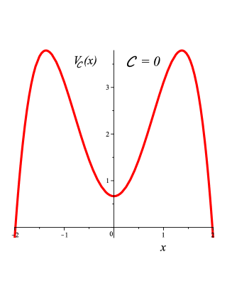
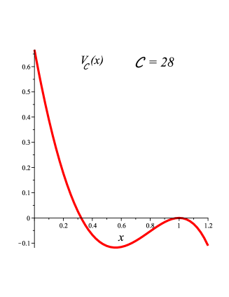
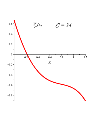
Figure 1. The graph of $V_{\mathcal{C}}$ for $\mathcal{C}=0,0<\mathcal{C}<10\sqrt{10}$ and $\mathcal{C}\geq 10\sqrt{10}$

Solutions of (3.5) satisfy the Hamiltonian identity

$$\frac{1}{2}(v^{\prime})^{2}+V_{\mathcal{C}}(v)=H,$$

where $H$ is a constant which depends on the initial data. The latter equation clearly implies that solutions of (3.5) also satisfy the first order ODE

(3.7) $$v^{\prime}=\pm\sqrt{2}\sqrt{H-V_{\mathcal{C}}(v)},$$

where the $\pm$ sign switches each time $v^{\prime}$ vanishes and $v^{\prime\prime}\neq 0$.

Case 1: $\mathcal{C}=0$

In this situation the potential $V_{\mathcal{C}}$ is even in $v$, and we can summarize the results in the following proposition.

Proposition 3.1.

(Existence of Delaunay-type solutions) There exist a one-parameter family of singular solutions $u_{\alpha}$ ($\alpha\in[0,1)$) to (3.1), periodic in $t$, and constants $C_{\alpha}>1$ such that

(3.8) $$\frac{1}{C_{\alpha}}\frac{(dx)^{2}}{|x|^{2}}\leq e^{2u_{\alpha}}(dx)^{2}\leq C_{\alpha}\frac{(dx)^{2}}{|x|^{2}}\qquad\quad\hbox{ for all }x\in\mathbb{R}^{4}.$$

For $\alpha=0$ we have $e^{2u_{0}(x)}\equiv\frac{1}{|x|^{2}}$.

Proof.  The existence of a one-parameter family of solutions follows easily from (3.5), using the fact that $V_{0}$ has a reversed double-well structure with two maxima at $v=\pm\mathrm{v}$, $\mathrm{v}=\frac{\sqrt{30}}{4}$. Their Hamiltonian energy $H$ ranges in the interval $\left[\frac{2}{3},\frac{91}{24}\right)$. For $H=\frac{2}{3}$ we have a constant solution $v_{0}\equiv 0$, corresponding to the function $u_{0}$ in the statement of the proposition.

For $H\in\left(\frac{2}{3},\frac{91}{24}\right)$ we obtain a periodic solution $v_{H}(t)$ oscillating between $-\mathfrak{v}_{H}$ and $\mathfrak{v}_{H}$, where $0<\mathfrak{v}_{H}<\mathrm{v}$. Since $v_{H}(t)$ stays uniformly bounded, we get (3.8) setting $\alpha=\frac{8}{25}(H-2/3)$.  

Remark 3.2.

When $H=\frac{91}{24}$ we obtain a heteroclinic orbit of (3.5) (with $\mathcal{C}=0$) connecting $-\mathrm{v}$ to $+\mathrm{v}$. On $\mathbb{R}^{4}\setminus\{0\}$, this corresponds to a solution to (3.1) giving rise to a metric proportional to $r^{-2(1+\mathrm{v})}(dx)^{2}$ near zero and to $r^{2(\mathrm{v}-1)}(dx)^{2}$ near infinity. These metrics resemble a Schwarzschild type solution but they are not asymptotically flat near zero or infinity: asymptotic flatness would correspond to $\mathrm{v}=1$.

It may help to clarify the preceding remark by considering an explicit example: if we take as our initial conditions $u^{\prime}(0)=0,u^{\prime\prime}(0)=5/2$, and $u^{\prime\prime\prime}(0)=0$, then a solution of (3.3) is given by

(3.9) $$u(t)=At+\frac{3}{4}\log\big{(}1+e^{-\frac{8}{3}At}\big{)},$$

where $A=\sqrt{\frac{15}{8}}>1$. Hence,

(3.10) $$g=e^{2At}\big{(}1+e^{-\frac{8}{3}At}\big{)}^{3/2}(dt^{2}+g_{S^{3}})$$

is a $U$-flat metric conformal to the cylinder. Performing the change of variable $r=\frac{1}{A}e^{At}$, we can write $g$ as

(3.11) $$g=[1+O(r^{-8/3})]\big{(}dr^{2}+A^{2}r^{2}g_{S^{3}}\big{)}.$$

Therefore, we see that near infinity, $g$ is asymptotic to a Euclidean cone.

Case 2: $0<\mathcal{C}<10\sqrt{10}$

In this case the potential $V_{\mathcal{C}}$ has two local maxima $\mathrm{v}_{1,\mathcal{C}}<0<\mathrm{v}_{2,\mathcal{C}}$, with $V(\mathrm{v}_{1,\mathcal{C}})>V(\mathrm{v}_{2,\mathcal{C}})$. We have the following proposition.

Proposition 3.3.

For $0<\mathcal{C}<10\sqrt{10}$ there exists a two-parameter family of solutions $u_{\mathcal{C},\alpha}$ ($\alpha\in[0,1]$) of (3.1) on $\mathbb{R}^{4}\setminus\{0\}$, periodic in $t$, and $C_{\mathcal{C},\alpha}>1$, $\beta_{\mathcal{C},\alpha}\in\mathbb{R}$ such that

(3.12) $$\frac{1}{C_{\mathcal{C},\alpha}}r^{2(\beta_{\mathcal{C},\alpha}-1)}(dx)^{2}\leq e^{2u_{\mathcal{C},\alpha}}(dx)^{2}\leq C_{\mathcal{C},\alpha}r^{2(\beta_{\mathcal{C},\alpha}-1)}(dx)^{2}\qquad\quad\hbox{ for all }x\in\mathbb{R}^{4}.$$

For $\mathcal{C}=28\in(0,10\sqrt{10})$ and $\alpha=1$ we have that $\beta_{\mathcal{C},\alpha}=1$, and the metric corresponding to $e^{2u_{28,1}}$ extends smoothly to (a non flat one on) $\mathbb{R}^{4}$.

Proof.  The proof of the existence part goes exactly as for the previous proposition, with the difference that when $\alpha=1$ we obtain a homoclinic solution (to $\mathrm{v}_{2,\mathcal{C}}$ for $t\to\pm\infty$) instead of a heteroclinic solution.

Let $u_{\mathcal{C},\alpha}$ be as above and let $\alpha<1$: then $v_{\mathcal{C},\alpha}\equiv u^{\prime}_{\mathcal{C},\alpha}$ oscillates periodically (with period $T_{\mathcal{C},\alpha}$) between two values $\tilde{\mathrm{v}}_{\mathcal{C},\alpha},\hat{\mathrm{v}}_{\mathcal{C},\alpha}$, with $\hat{\mathrm{v}}_{\mathcal{C},\alpha}>0$. Suppose that for some $t$ one has

$$v_{\mathcal{C},\alpha}(t)=\tilde{\mathrm{v}}_{\mathcal{C},\alpha};\qquad\quad v_{\mathcal{C},\alpha}(t+T_{\mathcal{C},\alpha}/2)=\hat{\mathrm{v}}_{\mathcal{C},\alpha}.$$

Then, from (3.7) one finds

$$T_{\mathcal{C},\alpha}=2\int_{t}^{t+T_{\mathcal{C},\alpha}/2}ds=2\sqrt{2}\int_{\tilde{\mathrm{v}}_{\mathcal{C},\alpha}}^{\hat{\mathrm{v}}_{\mathcal{C},\alpha}}\frac{dv}{\sqrt{2(H(\alpha)-V_{\mathcal{C}}(v))}},$$

where $H(\alpha)$ stands for the Hamiltonian energy of the trajectory $v_{\mathcal{C},\alpha}$. The number $\beta_{\mathcal{C},\alpha}$ in the statement, which can be taken as the average slope of $u_{\mathcal{C},\alpha}$, is given by

$$\beta_{\mathcal{C},\alpha}=\frac{2}{T_{\mathcal{C},\alpha}}\int_{t}^{t+T_{\mathcal{C},\alpha}/2}v_{\mathcal{C},\alpha}(s)ds=\frac{1}{\int_{\tilde{\mathrm{v}}_{\mathcal{C},\alpha}}^{\hat{\mathrm{v}}_{\mathcal{C},\alpha}}\frac{dv}{\sqrt{2(H(\alpha)-V_{\mathcal{C}}(v))}}}\int_{\tilde{\mathrm{v}}_{\mathcal{C},\alpha}}^{\hat{\mathrm{v}}_{\mathcal{C},\alpha}}\frac{v\,dv}{\sqrt{2(H(\alpha)-V_{\mathcal{C}}(v))}}.$$

For $\alpha=1$ then the average of $v$ is simply $\mathrm{v}_{2,\mathcal{C}}$.

When $\mathcal{C}=28$ one can check that $\mathrm{v}_{2,\mathcal{C}}=1$, which also implies $\beta_{\mathcal{C},\alpha}=1$. For the original solution $u(r)$, this corresponds to asymptotics of the form $u_{28,1}(r)=C_{0}-C_{1}r^{2}+o(r^{2})$ near zero and $u_{28,1}(r)=C_{2}+C_{3}r^{-2}+o(r^{-2})$ near infinity. Notice that the flat Euclidean metric corresponds to $u(t)\equiv t\not\equiv u_{28,1}(t)$. This concludes the proof.  

Remark 3.4.

When $\alpha$ is small (depending on $\mathcal{C}$) then we can infer that $\beta_{\mathcal{C},\alpha}>0$ since $v_{\mathcal{C},\alpha}$ oscillates near the local minimum of $V_{\mathcal{C}}$, which is positive. The same conclusion looks plausible for all $\alpha\in(0,1]$.

Case 3: $\mathcal{C}\geq 10\sqrt{10}$

In this situation the potential $V_{\mathcal{C}}$ has only one critical point (a local maximum) $\mathrm{w}_{\mathcal{C}}<0$ for $\mathcal{C}>10\sqrt{10}$, and two critical points $\mathrm{w}_{1}<0<\mathrm{w}_{2}$ for $\mathcal{C}=10\sqrt{10}$, respectively a local maximum and an inflection point. From this structure, one can easily see that all the globally defined solutions must be constants and coinciding with some stationary point of $\mathcal{V}_{\mathcal{C}}$.

4. The proof of Theorem 1.3

This Section we prove Theorem 1.3 for the case of the determinant of the Paneitz operator $F_{P}$. In Section 5 we indicate the necessary changes to prove the result for the half-torsion $F_{\tau}$.

Recall that the functional determinant for the Paneitz operator is

$$F_{P}[w]=-\frac{1}{4}I-14II+\frac{8}{3}III,$$

whose critical points satisfy the following Euler equation

(4.1) $$\begin{split}\mu e^{4w}&=9\Delta^{2}w+16\Delta|\nabla w|^{2}-32\nabla^{i}\big{[}(\Delta w+|\nabla w|^{2})\nabla_{i}w\big{]}-14R_{ij}\nabla_{i}\nabla_{j}w\\ &\hskip 18.06749pt+10R\Delta w+3\langle\nabla R,\nabla w\rangle-\frac{1}{4}|W|^{2}-14Q-\frac{8}{3}\Delta R,\end{split}$$

where

$$\mu=-\frac{\frac{1}{4}\int|W|^{2}+14\int Q}{\int e^{4w}}.$$

We will look for solutions on $S^{4}$ which are radial along some direction and symmetric with respect to a plane (orthogonal to this given direction), so it will still be convenient to set up the problem on the cylinder $\mathfrak{C}$, see the beginning of Section 3. Recall that on $\mathfrak{C}$ one has $R\equiv 6$ and $Q\equiv 0$ and (3.2), so if we look for solutions with total volume equal to $\frac{8}{3}\pi^{2}$ (the volume one of $S^{4}$) from (4.1) the Euler-Lagrange equation becomes the ordinary differential equation

(4.2) $$9u^{{}^{\prime\prime\prime\prime}}-96u^{\prime\prime}(u^{\prime})^{2}+60u^{\prime\prime}+42e^{4u}=0.$$

¿From the evenness of $u$ we require the initial conditions

(4.3) $$\left\{\begin{array}[]{ll}u^{\prime}(0)&=0,\\ u^{\prime\prime\prime}(0)&=0.\end{array}\right.$$

Since we need $u$ to lift to a solution on $S^{4}$ with the correct volume, we also need the asymptotic conditions

(4.4) $$u^{\prime\prime}(t)\rightarrow 0,\quad u^{\prime}(t)\rightarrow-1,\quad\int_{0}^{t}e^{4u}\ ds\rightarrow\frac{2}{3},\qquad\ t\rightarrow\infty.$$

4.1. An auxiliary equation

Using some algebra, we can show that (4.2) reduces to a third order equation without exponential terms.

Proposition 4.1.

Solutions of (4.2) such that (4.3) and (4.4) hold satisfy

(4.5) $$-\frac{9}{2}[u^{\prime\prime}(0)]^{2}+\frac{21}{2}e^{4u(0)}=6,$$

and also the equation

(4.6) $$\frac{9}{4}u^{\prime\prime\prime\prime}-9u^{\prime}u^{\prime\prime\prime}-24u^{\prime\prime}(u^{\prime})^{2}+\frac{9}{2}(u^{\prime\prime})^{2}+15u^{\prime\prime}+24(u^{\prime})^{4}-30(u^{\prime})^{2}+6=0.$$

Proof.  One can integrate (4.2) and use the initial conditions (4.3) to get a third order relation:

(4.7) $$9u^{\prime\prime\prime}-32(u^{\prime})^{3}+60u^{\prime}+42\int_{0}^{t}e^{4u}\ ds=0.$$

Now, multiplying this equation by $u^{\prime\prime}$ and integrating from $0$ to $t$, integrating by parts in the last term, and using the initial conditions (4.3) again, we get

(4.8) $$\frac{9}{2}(u^{\prime\prime})^{2}-\frac{9}{2}[u^{\prime\prime}(0)]^{2}-8(u^{\prime})^{4}+30(u^{\prime})^{2}+42u^{\prime}\int^{t}_{0}e^{4u}\ ds-\frac{21}{2}\big{[}e^{4u}-e^{4u(0)}\big{]}=0.$$

Substituting (4.4) into (4.8) gives then (4.5).

Putting this back into (4.8) holds

(4.9) $$\frac{9}{2}(u^{\prime\prime})^{2}-8(u^{\prime})^{4}+30(u^{\prime})^{2}+42u^{\prime}\int^{t}_{0}e^{4u}\ ds-\frac{21}{2}e^{4u}+6=0.$$

Let us now use (4.7) to write

$$42\int_{0}^{t}e^{4u}\ ds=-9u^{\prime\prime\prime}+32(u^{\prime})^{3}-60u^{\prime},$$

which implies

(4.10) $$42u^{\prime}\int_{0}^{t}e^{4u}\ ds=-9u^{\prime}u^{\prime\prime\prime}+32(u^{\prime})^{4}-60(u^{\prime})^{2}.$$

Likewise, use the original equation (4.2) to find

(4.11) $$-\frac{21}{2}e^{4u}=\frac{9}{4}u^{{}^{\prime\prime\prime\prime}}-24u^{\prime\prime}(u^{\prime})^{2}+15u^{\prime\prime}.$$

Substituting these into (4.9), we eliminate the exponential terms, and get (4.6).  

Remark 4.2.

Putting together (4.7) and (4.9) one also finds the conservation law

(4.12) $$9u^{\prime\prime\prime}u^{\prime}-\frac{9}{2}(u^{\prime\prime})^{2}-24(u^{\prime})^{4}+30(u^{\prime})^{2}+\frac{21}{2}e^{4u}=6.$$

By Proposition 4.1 and (4.3), if we let

$$x=x(t)=-u^{\prime}(t),$$

we get the ordinary differential equation

(4.13) $$\left\{\begin{array}[]{lll}x^{\prime\prime\prime}&=&-4xx^{\prime\prime}+\frac{32}{3}x^{2}x^{\prime}+2(x^{\prime})^{2}-\frac{20}{3}x^{\prime}+\frac{32}{3}x^{4}-\frac{40}{3}x^{2}+\frac{8}{3},\\ x(0)&=&0,\\ x^{\prime}(0)&=&-u^{\prime\prime}(0),\\ x^{\prime\prime}(0)&=&0.\end{array}\right.$$

Let us rewrite (4.13) as a first order system: define

$$\left\{\begin{array}[]{lll}y(t)&=&x^{\prime}(t),\\ z(t)&=&x^{\prime\prime}(t).\end{array}\right.$$

Then (4.13) is equivalent to

$$\left\{\begin{array}[]{lll}x^{\prime}&=&y,\\ y^{\prime}&=&z,\\ z^{\prime}&=&-4xz+\frac{32}{3}x^{2}y+2y^{2}-\frac{20}{3}y+\frac{32}{3}x^{4}-\frac{40}{3}x^{2}+\frac{8}{3}.\end{array}\right.$$

After some manipulation, we can rewrite this as

(4.14) $$\left\{\begin{array}[]{lll}x^{\prime}&=&y,\\ y^{\prime}&=&z,\\ z^{\prime}&=&\frac{32}{3}(x-1)\left(x-\frac{1}{2}\right)(x+1)\left(x+\frac{1}{2}\right)-4xz+2y^{2}+\frac{32}{3}x^{2}y-\frac{20}{3}y,\end{array}\right.$$

with initial conditions

(4.15) $$\left\{\begin{array}[]{lll}x(0)&=&0,\\ y(0)&=&-u^{\prime\prime}(0),\\ z(0)&=&0.\end{array}\right.$$

4.2. Some analysis of (4.14)

One can easily solve for the stationary points of (4.14): to begin, putting the first two components equal to zero implies that $y=z=0$. Plugging this into the third equation and setting it equal to zero gives

$$\frac{32}{3}(x-1)\left(x-\frac{1}{2}\right)(x+1)\left(x+\frac{1}{2}\right)=0.$$

Therefore,

$$(x,y,z)\hbox{ is stationary}\quad\Leftrightarrow\quad(x,y,z)=(\pm 1,0,0),\left(\pm\frac{1}{2},0,0\right).$$

Let

$$p_{0}=\left(\frac{1}{2},0,0\right),\qquad\qquad p_{1}=(1,0,0),$$

and let us look at the linearized system at each of these two critical points.

1. At $p_{1}$, letting $H(x,y,z)=\frac{32}{3}(x-1)\left(x-\frac{1}{2}\right)(x+1)\left(x+\frac{1}{2}\right)-4xz+2y^{2}+\frac{32}{3}x^{2}y-\frac{20}{3}y$, we have

$$\left\{\begin{array}[]{ll}\frac{\partial H}{\partial x}(p_{1})&=16,\\ \frac{\partial H}{\partial y}(p_{1})&=4,\\ \frac{\partial H}{\partial z}(p_{1})&=-4.\\ \end{array}\right.$$

Therefore, the linearized system at $p_{1}$ is

$$\left\{\begin{array}[]{ll}x^{\prime}(t)&=y,\\ y^{\prime}(t)&=z,\\ z^{\prime}(t)&=16x+4y-4z,\end{array}\right.$$

which we write as

$$\frac{d}{dt}X={\bf A_{1}}X,$$

with

(4.16) $$X=\left(\begin{array}[]{c}x\\ y\\ z\\ \end{array}\right);\qquad\qquad\quad{\bf A_{1}}=\left(\begin{array}[]{ccc}0&1&0\\ 0&0&1\\ 16&4&-4\end{array}\right).$$

The eigenvalues and eigenvectors are

(4.17) $${\bf A_{1}}{\bf v}_{1}=2{\bf v}_{1};\qquad\quad{\bf A_{1}}{\bf v}_{2}=-2{\bf v}_{2};\qquad\quad{\bf A_{1}}{\bf v}_{3}=-4{\bf v}_{3},\qquad\quad$$

where

$${\bf v}_{1}=\left(\begin{array}[]{c}1\\ 2\\ 4\\ \end{array}\right)\qquad\quad{\bf v}_{2}=\left(\begin{array}[]{c}1\\ -2\\ 4\\ \end{array}\right);\quad\qquad{\bf v}_{3}=\left(\begin{array}[]{c}1\\ -4\\ 16\\ \end{array}\right).$$

Therefore, $p_{1}$ is a saddle.

2. At $p_{0}$ we have

$$\left\{\begin{array}[]{ll}\frac{\partial H}{\partial x}(p_{0})&=-8,\\ \frac{\partial H}{\partial y}(p_{0})&=-4,\\ \frac{\partial H}{\partial z}(p_{0})&=-2,\\ \end{array}\right.$$

and the linearized system at this point is

$$\left\{\begin{array}[]{ll}x^{\prime}(t)&=y,\\ y^{\prime}(t)&=z,\\ z^{\prime}(t)&=-8x-4y-2z,\end{array}\right.$$

which we write as

$$\frac{d}{dt}X={\bf A_{0}}X,$$

with

$${\bf A_{0}}=\left(\begin{array}[]{ccc}0&1&0\\ 0&0&1\\ -8&-4&-2\end{array}\right).$$

The eigenvalues of this matrix are $\{-2,-2i,2i\}$: we will not need the explicit form of the eigenvectors.

The advantage of looking at system (4.13) instead of the original equation (4.2) is that it is an autonomous one in the derivatives. Moreover, it includes a one-parameter family of solutions to (3.4), which is a conservative version of (4.2).

Using our previous notation $(x,y,z)$, (3.4) becomes $K(x,y,z)=0$, where

$$K(x,y,z)=4-6xz+3y^{2}+16x^{4}-20x^{2}.$$

One can check that the set $\{K=0\}$ stays invariant for (4.13), and that solutions on this hypersurface also satisfy (3.4) with $v=-x$. Heuristically, if $u$ attains large negative values, one might expect that solutions of (4.2)-(4.4) (and hence of (4.12)) to behave like those of (3.4). In fact, this is what we will verify in Subsection 4.3 for suitable initial data, see also Remark 4.4 below.

We characterize a family of solutions to the first equation of (4.13) in the following proposition.

Proposition 4.3.

For $\mathcal{C}\in[26,28]$, define

$$F_{\mathcal{C}}(x,y,z)=y^{2}+2V_{\mathcal{C}}(x);\qquad\qquad G_{\mathcal{C}}(x,y,z)=z+\frac{d}{dx}V_{\mathcal{C}}(x),$$

where $V_{\mathcal{C}}$ is given in (3.6). Then for every $\mathcal{C}\in(26,28)$ the system

(4.18) $$\left\{\begin{array}[]{ll}F_{\mathcal{C}}(x,y,z)=0;&\\ G_{\mathcal{C}}(x,y,z)=0&\end{array}\right.$$

admits a periodic solution $X_{\mathcal{C}}$ which also satisfies

(4.19) $$x^{\prime\prime\prime}=-4xx^{\prime\prime}+\frac{32}{3}x^{2}x^{\prime}+2(x^{\prime})^{2}-\frac{20}{3}x^{\prime}+\frac{32}{3}x^{4}-\frac{40}{3}x^{2}+\frac{8}{3}.$$

We get the same conclusions regarding the constant solution $(x(t),y(t),z(t))\equiv p_{0}$ when $\mathcal{C}=26$, and also for an orbit homoclinic to $p_{1}$ at $t=\pm\infty$ when $\mathcal{C}=28$.

Proof.  Let us first discuss the existence of periodic solutions of (4.18). The equation $G_{\mathcal{C}}(x,y,z)=0$ is a Newton equation for $x(t)$ corresponding to the potential $V_{\mathcal{C}}$, while the function $F_{\mathcal{C}}$ stands for (twice) its Hamiltonian energy. ¿From the shape of the graph of $V_{\mathcal{C}}$, see Figure 2, it is easy to see that periodic solutions with zero Hamiltonian energy exist for $\mathcal{C}\in(26,28)$.

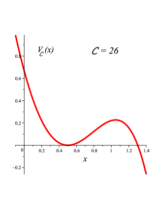
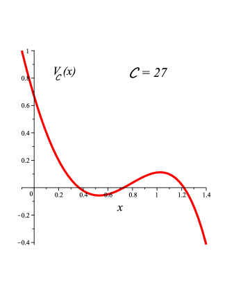
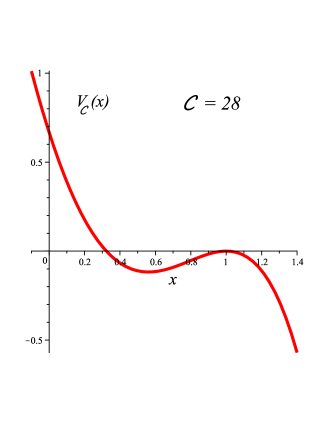
Figure 2. The graph of $V_{\mathcal{C}}$ for $\mathcal{C}=26,27,28$

The value $\mathcal{C}=28$ corresponds to a homoclinic solution $X_{0}=X_{\mathcal{C}=28}$ for which

$$X_{0}(t)\to p_{1}=(1,0,0)\qquad\quad\hbox{ as }t\to\pm\infty.$$

The value $\mathcal{C}=26$ instead characterizes the equilibrium point $p_{0}$ defined above.

By explicit substitution one can easily check that solutions of (4.18) also satisfy (4.19).  

As $\mathcal{C}$ varies between $26$ and $28$, the trajectories of $X_{\mathcal{C}}$ foliate a topological disk $\mathcal{D}$ in $\mathbb{R}^{3}$ whose boundary is the homoclinic orbit $X_{\mathcal{C}=28}$, and whose center is the point $p_{0}$, see Figure 3.

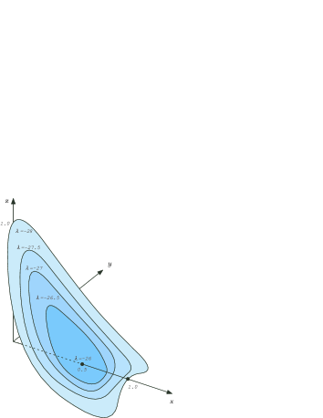
Figure 3. The topological disc $\mathcal{D}$

Let us now go back to equation (4.14). By some elementary algebra we obtain the following evolution equations along solutions

(4.20) $$\frac{d}{dt}F_{\mathcal{C}}=2yG_{\mathcal{C}};\qquad\quad\frac{d}{dt}G_{\mathcal{C}}=\frac{2}{3}K;\qquad\quad\frac{d}{dt}K=-4xK.$$

Remark 4.4.

At the points of the disc where $\nabla K\neq 0$ the last equation in (4.20) means that the flow is approaching $\mathcal{D}$ (which is contained in the zero level set of $K$) perpendicularly, so one could speculate there might exist a positive (in time) invariant set for (4.14). This will indeed be proven rigorously in Subsection 4.3.

We also consider the function

(4.21) $$Q(x,y,z)=-9z+32x^{3}-60x.$$

On the disk $\mathcal{D}$, $Q(x,y,z)$ coincides with $-\mathcal{C}$, considered as a variable selecting the periodic trajectory. Therefore, $\mathcal{D}\subseteq\mathbb{R}^{3}$ can be characterized as

$$\mathcal{D}=\{K=0\}\cap\{-28\leq Q\leq-26\}\cap\{0\leq x\leq 1\}.$$

The function $Q$ satisfies the ordinary differential equation

(4.22) $$\frac{d}{dt}Q=-6K.$$

Notice that $Q$ coincides with $-9G_{\mathcal{C}}-\mathcal{C}$, so $\frac{d}{dt}Q$ and $\frac{d}{dt}G_{\mathcal{C}}$ along solution have similar expressions.

4.3. Global existence near the spherical metric

On the cylinder $\mathfrak{C}$, the round metric corresponds to the conformal factor

(4.23) $$u_{0}(t)=-\log\cosh t=\log\left(\frac{2}{e^{t}+e^{-t}}\right),$$

which satisfies the initial conditions

(4.24) $$\left\{\begin{array}[]{ll}u_{0}^{\prime}(0)&=0,\\ u_{0}^{\prime\prime}(0)&=-1,\\ u_{0}^{\prime\prime\prime}(0)&=0.\end{array}\right.$$

The goal of this subsection is to show that for initial data

$$\left\{\begin{array}[]{ll}x(0)&=0,\\ y(0)&=1-\varepsilon,\\ z(0)&=0,\end{array}\right.$$

with $\varepsilon>0$ small, the solution of (4.14) is globally defined, and hence also the solution of (4.2).

Let us set

(4.25) $$\mathcal{N}[u]=9u^{{}^{\prime\prime\prime\prime}}-96u^{\prime\prime}(u^{\prime})^{2}+60u^{\prime\prime}+42e^{4u},$$

so that solutions $u$ of (4.2) are characterized by $\mathcal{N}[u]=0.$ Let $\mathcal{L}$ denote the linearized operator

(4.26) $$\mathcal{L}_{u}\phi=\frac{d}{ds}\mathcal{N}[u+s\phi]\Big{|}_{s=0}.$$

If $u=u_{0}$ is the standard bubble then we simply denote $\mathcal{L}_{u_{0}}$ by $\mathcal{L}_{0}$. An easy calculation gives

(4.27) $$\mathcal{L}_{0}[\phi]=9\phi^{\prime\prime\prime\prime}+[60-96(\tanh t)^{2}]\phi^{\prime\prime}-192(\hbox{sech}t)^{2}(\tanh t)\phi^{\prime}+168(\hbox{sech}t)^{4}\phi.$$

As $t\rightarrow\infty$, this limits to the equation

(4.28) $$\mathcal{L}_{0}\phi\sim 9\phi^{\prime\prime\prime\prime}-36\phi^{\prime\prime},$$

so one should expect $\phi$ to be of exponential type at infinity.

Indeed, if we linearize the initial conditions on $u$ (4.5), on $\phi$ we have to impose

$$\phi(0)=-\frac{3}{14};\qquad\phi^{\prime}(0)=0;\qquad\phi^{\prime\prime}(0)=1;\qquad\phi^{\prime\prime\prime}(0)=0.$$

An explicit solution is given by the following formula (see Chapter 15 in [AS64] for definitions and properties of hypergeometric functions)

$$\phi(t)=-\frac{3}{14}\hbox{hypergeom}\left(\left[\frac{3}{4}-\frac{1}{12}\sqrt{249},\frac{3}{4}+\frac{1}{12}\sqrt{(}249)\right],\frac{1}{2},\cos(2\arctan(e^{t}))^{2}\right).$$

By the asymptotics of hypergeometric functions, as $t$ tends to infinity one has

(4.29) $$\phi(t)=A(e^{2t}+O(1));\qquad\qquad\phi^{\prime}(t)=2A(e^{2t}+O(1));$$

(4.30) $$\phi^{\prime\prime}(t)=4A(e^{2t}+O(1));\qquad\qquad\phi^{\prime\prime\prime}(t)=8A(e^{2t}+O(1))$$

for some $A>0$, where $O(1)$ is a quantity which stays uniformly bounded as $t\to+\infty$.

We prove first the following result, yielding existence for an interval in the variable $t$ which grows as $\varepsilon\to 0$, and which relies on a Gronwall type inequality.

Proposition 4.5.

Given $\delta>0$ sufficiently small, there exists $\varepsilon_{0}>0$ such that, for $\varepsilon\in(0,\varepsilon_{0})$ the solution of the system with initial data

$$(x(0),y(0),z(0))=(0,1-\varepsilon,0)$$

is defined up to $t=\log\delta-\frac{1}{2}\log\varepsilon$, and one has the estimates

(4.31) $$\left\{\begin{array}[]{ll}\left|x(t)-1+2(e^{-2t}+\varepsilon Ae^{2t})\right|\leq\delta\varepsilon Ae^{2t};&\\ &\\ \left|y(t)-4(e^{-2t}-\varepsilon Ae^{2t})\right|\leq\delta\varepsilon Ae^{2t};&\\ &\\ \left|z(t)+8(e^{-2t}+\varepsilon Ae^{2t})\right|\leq\delta\varepsilon Ae^{2t},&\end{array}\right.\qquad\hbox{ for }t\in\left[-\log\delta,\log\delta-\frac{1}{2}\log\varepsilon\right],$$

where $A$ is as in (4.29) and (4.30).

Proof.  We can use a Gronwall inequality for the difference between the true solution and an approximate one. Calling $\varphi$ the solution to the linearized equation, we set $x^{\varepsilon}(t)=x^{0}(t)+\varepsilon\varphi(t)+\tilde{x}^{\varepsilon}(t)$ and then write a differential inequality for $\tilde{x}^{\varepsilon}$. Recalling that

$$X(t)=(x(t),y(t),z(t)),$$

we write (4.14) in the vector form

$$\frac{d}{dt}X(t)=F(X).$$

We begin by considering the trajectory $X^{0}$ corresponding to the spherical metric (for $\varepsilon=0$), which satisfies

(4.32) $$\frac{d}{dt}{X}^{0}=F(X^{0});\qquad\quad X^{0}(0)=(0,1,0).$$

Given a large but fixed $t_{0}$, by (4.23) we have

(4.33) $$\left\{\begin{array}[]{ll}X^{0}_{1}(t_{0})&=1-2e^{-2t_{0}}+O(e^{-4t_{0}});\\ X^{0}_{2}(t_{0})&=4e^{-2t_{0}}+O(e^{-4t_{0}});\\ X^{0}_{3}(t_{0})&=-8e^{-2t_{0}}+O(e^{-4t_{0}}).\end{array}\right.$$

When we linearize in $\varepsilon$ the equation for initial data $X^{\varepsilon}(0)=(0,1-\varepsilon,0)$, the linearized solution satisfies

(4.34) $$\frac{d}{dt}\varphi=F^{\prime}(X^{0})[\varphi],$$

with initial conditions $\varphi(0)=(0,-1,0)$. Recall that, by our previous notation from Subsection 4.3 we have

(4.35) $$\varphi_{1}=-\phi^{\prime};\qquad\qquad\varphi_{2}=-\phi^{\prime\prime};\qquad\qquad\varphi_{3}=-\phi^{\prime\prime\prime},$$

so from (4.29) and (4.30) we find

$$X^{\varepsilon}_{1}(t_{0})=1-2e^{-2t_{0}}-2A\varepsilon e^{2t_{0}}+O(\varepsilon^{2});\qquad\qquad X_{2}^{\varepsilon}(t_{0})=4e^{-2t_{0}}-4\varepsilon Ae^{2t_{0}}+O(\varepsilon^{2});$$

$$X_{3}^{\varepsilon}(t_{0})=-8e^{-2t_{0}}-8\varepsilon Ae^{2t_{0}}+O(\varepsilon^{2}).$$

Here, $O(\varepsilon^{2})$ stands for a quantity bounded by $C_{t_{0}}\varepsilon^{2}$. We now choose $\delta>0$ (small but fixed), and then $t_{0}$ to be the first value of $t$ (depending on $\delta$) such that $X^{\varepsilon}_{1}(t_{0})=\frac{\delta}{32}$. In this way, we can write indirectly that $C_{t_{0}}=C_{\delta}$.

We next set

$$X^{\varepsilon}=X^{0}+\varepsilon\varphi+\tilde{X}^{\varepsilon},$$

and from a Taylor expansion we find

$$\left\|F(X^{\varepsilon})-F(X^{0})-\varepsilon F^{\prime}(X_{0})[\varphi]-F^{\prime}(X^{0})[\tilde{X}^{\varepsilon}]\varphi\right\|\leq C_{1}\|\varepsilon\varphi+\tilde{X}^{\varepsilon}\|^{2},$$

where $C_{1}$ is a fixed positive constant (uniformly bounded as long as the solution lies in a fixed compact set of $\mathbb{R}^{3}$). Therefore, using the last formula and some cancelation, we find that

$$\left\|\frac{d}{dt}\tilde{X}^{\varepsilon}-F^{\prime}(X^{0})[\tilde{X}^{\varepsilon}]\right\|\leq C_{1}\|\varepsilon\varphi+\tilde{X}^{\varepsilon}\|^{2}.$$

This implies

$$\|\tilde{X}^{\varepsilon}\|\frac{d}{dt}\|\tilde{X}^{\varepsilon}\|=\frac{1}{2}\frac{d}{dt}\|\tilde{X}^{\varepsilon}\|^{2}=\langle\tilde{X}^{\varepsilon},\frac{d}{dt}\tilde{X}^{\varepsilon}\rangle\leq\langle F^{\prime}(X^{0})[\tilde{X}^{\varepsilon}],\tilde{X}^{\varepsilon}\rangle+C_{1}\|\varepsilon\varphi+\tilde{X}^{\varepsilon}\|^{2}\|\tilde{X}^{\varepsilon}\|,$$

and hence

(4.36) $$\frac{d}{dt}\|\tilde{X}^{\varepsilon}\|\leq\frac{\langle F^{\prime}(X^{0})[\tilde{X}^{\varepsilon}],\tilde{X}^{\varepsilon}\rangle}{\|\tilde{X}^{\varepsilon}\|}+C_{1}\|\varepsilon\varphi+\tilde{X}^{\varepsilon}\|^{2}.$$

Recalling that $F^{\prime}(0)={\bf A_{1}}$, see (4.16), since $F$ is Lipschitz by (4.33) one has

$$\left\|F^{\prime}(X^{0})-{\bf A_{1}}\right\|\leq C_{1}\|X^{0}\|\leq\frac{\delta}{2}\qquad\quad\hbox{ as long as }\quad e^{-2t}\leq\frac{\delta}{1000\,C_{1}}.$$

By (4.17) this implies

$$\frac{\langle F^{\prime}(X^{0})[\tilde{X}^{\varepsilon}],\tilde{X}^{\varepsilon}\rangle}{\|\tilde{X}^{\varepsilon}\|} \leq \frac{\langle{\bf A_{1}}[\tilde{X}^{\varepsilon}],\tilde{X}^{\varepsilon}\rangle}{\|\tilde{X}^{\varepsilon}\|}+\frac{\delta}{2}\|\tilde{X}^{\varepsilon}\|$$

$$\leq \left(2+\frac{\delta}{2}\right)\|\tilde{X}^{\varepsilon}\|\qquad\hbox{ as long as }\quad e^{-2t}\leq\frac{\delta}{1000\,C_{1}}.$$

¿From (4.36) we then get

$$\frac{d}{dt}\|\tilde{X}^{\varepsilon}\|\leq\left(2+\frac{\delta}{2}\right)\|\tilde{X}^{\varepsilon}\|+C_{1}\|\varepsilon\varphi\|^{2}+2C_{1}\|\varepsilon\varphi\|\,\|\tilde{X}^{\varepsilon}\|+C_{1}\|\tilde{X}^{\varepsilon}\|^{2},$$

which by (4.35) and (4.29), (4.30) yields

$$\frac{d}{dt}\|\tilde{X}^{\varepsilon}\|\leq 2(1+\delta)\|\tilde{X}^{\varepsilon}\|+C_{1}\|\varepsilon\varphi\|^{2}\qquad\hbox{ as long as }\qquad\left\{\begin{array}[]{ll}e^{-2t}+\varepsilon Ae^{2t}\leq\frac{\delta}{1000\,C_{1}};&\\ \|\tilde{X}^{\varepsilon}\|\leq\frac{\delta}{1000\,C_{1}}.&\end{array}\right.$$

Therefore, by the asymptotic behavior of $\varphi$ we have that

(4.37) $$\frac{d}{dt}\|\tilde{X}^{\varepsilon}\|\leq 2(1+\delta)\|\tilde{X}^{\varepsilon}\|+128C_{1}\varepsilon^{2}e^{4t}\qquad\hbox{ as long as }\qquad\left\{\begin{array}[]{ll}e^{-2t}+\varepsilon Ae^{2t}\leq\frac{\delta}{1000\,C_{1}};&\\ \|\tilde{X}^{\varepsilon}\|\leq\frac{\delta}{1000\,C_{1}}.&\end{array}\right.$$

By solving explicitly the associated differential equality, the solution of (4.37) with an initial condition such that $\|\tilde{X}^{\varepsilon}\|(t_{0})\leq C_{\delta}\varepsilon^{2}$ then verifies

$$\|\tilde{X}^{\varepsilon}\|(t)\leq C_{\delta}\varepsilon^{2}e^{2(1+\delta)(t-t_{0})}-\frac{C_{1}\varepsilon^{2}}{2(1-\delta)}e^{2(1+\delta)(t-t_{0})}+\frac{C_{1}\varepsilon^{2}}{2(1-\delta)}e^{4(t-t_{0})}$$

recall, as long as

(4.38) $$e^{-2t}+\varepsilon Ae^{2t}\leq\frac{\delta}{1000\,C_{1}}\qquad\quad\hbox{ and }\qquad\quad\|\tilde{X}^{\varepsilon}\|\leq\frac{\delta}{1000\,C_{1}}.$$

We next check the latter condition for $t\in\left[-\log\delta,\log\delta-\frac{1}{2}\log\varepsilon\right]$. In fact, for $t$ in this range we have that

$$e^{-2t}\leq\delta^{2}<\frac{\delta}{1000\,C_{1}};\qquad\qquad\varepsilon Ae^{2t}\leq A\delta^{2}<\frac{\delta}{1000\,C_{1}},$$

provided we choose initially $\delta$ sufficiently small.

Concerning the second inequality in (4.38), for $t\in\left[-\log\delta,\log\delta-\frac{1}{2}\log\varepsilon\right]$ we get

$$\|\tilde{X}^{\varepsilon}\|(t)\leq C_{\delta}\varepsilon^{2}\left(\frac{\delta^{2}}{\varepsilon}\right)^{1+\delta}+C_{1}\varepsilon^{2}\frac{\delta^{4}}{\varepsilon^{2}}=C_{\delta}\delta^{2(1+\delta)}\varepsilon^{1-\delta}+C_{1}\delta^{4}<\frac{\delta}{1000\,C_{1}},$$

provided $\delta$ is small enough, and if $\varepsilon\to 0$. The last estimate also shows that, for $t$ in the interval $\left[-\log\delta,\log\delta-\frac{1}{2}\log\varepsilon\right]$

$$\|\tilde{X}^{\varepsilon}\|(t)\leq\left(C_{\delta}\delta^{2\delta-1}\varepsilon^{1-\delta}+C_{1}\delta^{2}\right)\varepsilon e^{2t}<\delta\varepsilon Ae^{2t}$$

for $\delta$ sufficiently small, which is the desired conclusion.  

We will show next that, for suitable initial data close to the ones of the standard bubble, there exists a globally defined trajectory.

Proposition 4.6.

For $\varepsilon>0$ small enough the solution $X^{\varepsilon}$ of (4.14) with initial data

(4.39) $$X^{\varepsilon}(0)=(0,1-\varepsilon,0)$$

is globally defined and there exists $\Lambda_{\varepsilon}\in(-28,-26]$ such that

$$K(X(t))\to 0,\qquad Q(X(t))\to\Lambda_{\varepsilon}\qquad\qquad\hbox{ as }\qquad t\to+\infty.$$

Moreover, as $t\to+\infty$, $X^{\varepsilon}$ becomes asymptotically periodic.

Proof.  By Proposition 4.5, there is $\delta$ is sufficiently small such that, if $\varepsilon\to 0$, the solution $X^{\varepsilon}$ is defined at least up to $t=\log\delta-\frac{1}{2}\log\varepsilon$. Evaluating it for $\tilde{t}_{\varepsilon}:=-\frac{1}{4}\log\varepsilon-\frac{1}{4}\log A$ (which is in the interval where (4.31) holds), one has that

$$x(\tilde{t}_{\varepsilon})=1-4e^{-2\tilde{t}_{\varepsilon}}+2e^{-4\tilde{t}_{\varepsilon}}+R_{1};\qquad\quad y(\tilde{t}_{\varepsilon})=4e^{-2\tilde{t}_{\varepsilon}}-8e^{-4\tilde{t}_{\varepsilon}}+R_{2};$$

$$z(\tilde{t}_{\varepsilon})=-16e^{-2\tilde{t}_{\varepsilon}}+32e^{-4\tilde{t}_{\varepsilon}}+R_{3},$$

where

$$|R_{i}|\leq\delta\varepsilon Ae^{2\tilde{t}_{\varepsilon}}=\delta e^{-2\tilde{t}_{\varepsilon}}.$$

¿From some elementary expansions one finds that

$$(Q+28)(\tilde{t}_{\varepsilon})=1320e^{-4\tilde{t}_{\varepsilon}}+36R_{1}-9R_{3}+\tilde{R}_{Q};$$

$$K(\tilde{t}_{\varepsilon})=688e^{-4\tilde{t}_{\varepsilon}}+24R_{1}-6R_{3}+\tilde{R}_{K},$$

where $|\tilde{R}_{Q}|+|\tilde{R}_{K}|\leq C_{2}\delta\varepsilon A$, for a fixed constant $C_{2}>0$. In particular, setting

$$f(t)=\frac{(Q+28)(t)}{K(t)},$$

one has $f(t_{\varepsilon})>\frac{3}{2}+\tilde{C}_{\delta}e^{-2\tilde{t}_{\varepsilon}}$, where $\tilde{C}_{\delta}\to+\infty$ as $\delta\to 0$. Using (4.20) and (4.22) one finds that

(4.40) $$\frac{d}{dt}f(t)=4x(t)f(t)-6.$$

We now estimate the solution from below: setting

$$h(t)=\frac{3}{2}+\left(f(\tilde{t}_{\varepsilon})-\frac{3}{2}\right)e^{3(t-\tilde{t}_{\varepsilon})},$$

we show that $h(t)$ is a subsolution of the equation. Since for $t\geq\tilde{t}_{\varepsilon}$ one has $\varepsilon Ae^{2t}\geq e^{-2t}$, from the estimates we have on $x(t)$ this would be satisfied if

$$3\left(f(\tilde{t}_{\varepsilon})-\frac{3}{2}\right)e^{3(t-\tilde{t}_{\varepsilon})}\leq 4(1-8\varepsilon Ae^{2t})\left(\frac{3}{2}+\left(f(\tilde{t}_{\varepsilon})-\frac{3}{2}\right)e^{3(t-\tilde{t}_{\varepsilon})}\right)-6,$$

namely if

$$32A\varepsilon e^{2t}\left(1+C_{\delta}e^{3t-5\tilde{t}_{\varepsilon}}\right)\leq C_{\delta}e^{3t-5\tilde{t}_{\varepsilon}}\qquad\hbox{ for }t\geq\tilde{t}_{\varepsilon}.$$

We claim that this is true for $\tilde{t}_{\varepsilon}\leq t\leq\frac{1}{2}\log\frac{\delta^{4}}{\varepsilon A}$. Notice that this number is smaller than $\log\delta-\frac{1}{2}\log\varepsilon$, and the estimates of Proposition 4.5 hold true. We prove that separately

$$32A\varepsilon e^{2t}\leq\frac{1}{2}C_{\delta}e^{3t-5\tilde{t}_{\varepsilon}}\qquad\hbox{ and }\qquad 32A\varepsilon C_{\delta}e^{5t-5\tilde{t}_{\varepsilon}}\leq\frac{1}{2}C_{\delta}e^{3t-5\tilde{t}_{\varepsilon}};\qquad\quad t\leq\frac{1}{2}\log\frac{\delta^{4}}{\varepsilon A}.$$

Taking into account that $e^{-4\tilde{t}_{\varepsilon}}=\varepsilon A$, the first inequality is equivalent to

$$C_{\delta}e^{t-\tilde{t}_{\varepsilon}}\geq 64,$$

which is true for $\delta$ small (recall that $C_{\delta}\to+\infty$ as $\delta\to 0$). The second inequality is instead equivalent to

$$64A\varepsilon e^{2t}\leq 1,$$

but since $t\leq\frac{1}{2}\log\frac{\delta^{4}}{\varepsilon A}$ we have

$$64A\varepsilon e^{2t}\leq 64\delta^{4},$$

which is true for $\delta$ small. Therefore, we proved that $h(t)$ is a subsolution.

Hence by comparison we find

$$f\left(\frac{1}{2}\log\frac{\delta^{4}}{\varepsilon A}\right)\geq h\left(\frac{1}{2}\log\frac{\delta^{4}}{\varepsilon A}\right)\geq\frac{3}{2}+C_{\delta}e^{-5\tilde{t}_{\varepsilon}}\frac{\delta^{6}}{(\varepsilon A)^{\frac{3}{2}}}.$$

Using the choice of $\tilde{t}_{\varepsilon}$ then we obtain

$$f\left(\frac{1}{2}\log\frac{\delta^{4}}{\varepsilon A}\right)\geq\frac{3}{2}+C_{\delta}(\varepsilon A)^{\frac{5}{4}}\frac{\delta^{6}}{(\varepsilon A)^{\frac{3}{2}}}\geq C_{\delta}\delta^{6}(\varepsilon A)^{-\frac{1}{4}}.$$

This means that

(4.41) $$\hbox{ for any }M>0\hbox{ there exists }t_{\varepsilon,M}>\tilde{t}_{\varepsilon}\hbox{ such that }f(t)=M.$$

Now we notice that

(4.42) $$W(x,y):=4+20x^{2}-\frac{16}{3}x^{4}+3y^{2}-\frac{56}{3}x=K-\frac{2}{3}x(Q+28)=\frac{2}{3}K\left(\frac{3}{2}-xf\right).$$

At $t_{\varepsilon,M}$ the right hand side is negative. On the other hand $\{W<0\}\subseteq\mathbb{R}^{2}$ has a bounded component $W_{0}$ contained in

$$(x,y)\in\left[\frac{1}{5},1\right]\times\left[-\frac{3}{5},\frac{3}{5}\right],$$

(see Figure 4) and $(x(t_{\varepsilon,M}),y(t_{\varepsilon,M}))\in W_{0}$.

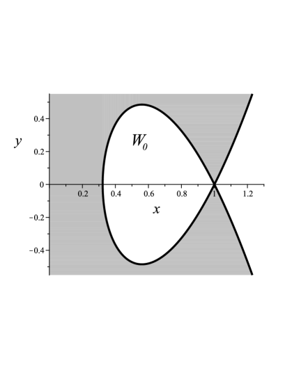
Figure 4. The components of $\{W<0\}$ (in white)

Therefore, as long as $\frac{3}{2}-x(t)f(t)<0$, we have a-priori bounds on $x(t)$ and $y(t)$, and $x(t)$ stays positive and bounded away from zero. Moreover, $K(t_{\varepsilon,M})$ is small positive. Using the expression of $K$ and the a-priori bounds on $x(t)$ and $y(t)$, one also finds a-priori bounds on $z(t)$, as long as $\frac{3}{2}-x(t)f<0$.

If we choose $M>300$ in (4.41), then $\frac{3}{2}-x(t_{\varepsilon,M})f<0$ so, by the bounds on $x(t)$ and by (4.40) $f$ will increase in $t$, so we obtain global existence if $\varepsilon>0$ is sufficiently small.

Since $x(t)$ stays bounded, positive and bounded away from zero, by (4.20) we find immediately that $K(t)\to 0$ as $t\to+\infty$. It remains to prove that $Q\to\Lambda_{\varepsilon}\in(-28,-26]$ as $t\to+\infty$. Notice that, since $K(0)>0$ and since $K(t)$ stays positive, $Q$ is monotone decreasing.

Now, for a small constant $\eta>0$ and large constant $B>0$ (to be chosen properly), we consider the set

(4.43) $$\Omega_{\eta,B}:=\left\{0\leq K\leq\frac{28-\eta+Q}{B}\right\}.$$

One has that $\nabla K\neq 0$ on $\{K=0\}\cap\{Q\in[-28,-26]\}$ (recall that $\mathcal{D}\subseteq\{K=0\}$ and the third equation in (4.20)), so for $B$ large and $\eta$ small $\Omega_{\eta,B}$ is a thin neighborhood of the set $\{K=0\}\cap\{-28+\eta\leq Q\leq-26\}$, on the side of $\{K\geq 0\}$.

Using (4.20) and (4.22) and the bounds on $x(t)$, one can check that if $B$ is large then $\Omega_{\eta,B}$ is positive invariant in $t$. Moreover, from the fact that $f(t)\to+\infty$ as $t\to+\infty$, we can find $t$ large and $\eta$ small such that $X(t)\in\Omega_{\eta,B}$. Since $Q(t)$ is monotone decreasing and since $Q\geq-28+\eta$ in $\Omega_{\eta,B}$, we obtain that $Q(t)\to\Lambda_{\varepsilon}\in(-28,26]$ as $t\to+\infty$, which is the desired conclusion.  

In Figure 5 a numerical solutions $X^{\varepsilon}$ of (4.14) is drawn, shadowing one of the periodic orbits in $\mathcal{D}$.

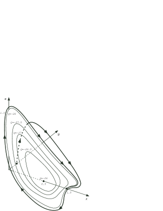
Figure 5. A solution of (4.14) approaching $\mathcal{D}$

4.4. A continuity argument

In this subsection we deform the value of the parameter $\varepsilon$ in (4.39) in order to obtain geometrically admissible solutions, namely the conditions in (4.4).

Given $\varepsilon>0$, we let $X^{\varepsilon}=(x^{\varepsilon}(t),y^{\varepsilon}(t),z^{\varepsilon}(t))$ denote the solution of (4.14) with initial condition (4.39), and we let $T(\varepsilon)$ be the largest number such that $X^{\varepsilon}$ is defined on $[0,T(\varepsilon))$. We then let $\mathcal{E}$ be the family of values of $\varepsilon\geq 0$ such that

$$\left\{\begin{array}[]{ll}T(\varepsilon)=+\infty;&\\ K(X^{\varepsilon}(t))\to 0&\hbox{ as }t\to+\infty;\\ Q(X^{\varepsilon}(t))\to\Lambda_{\varepsilon}\in[-28,-26]&\hbox{ as }t\to+\infty.\end{array}\right.$$

We also set

(4.44) $$\overline{\varepsilon}=\sup\left\{\tilde{\varepsilon}\;:\;[0,\tilde{\varepsilon}]\subseteq\mathcal{E}\right\}.$$

First, we show that $\overline{\varepsilon}$ is finite.

Lemma 4.7.

For $\varepsilon>0$ sufficiently large $T(\varepsilon)$ is finite, and hence $\overline{\varepsilon}<+\infty$.

Proof.  If we define

(4.45) $$\mathcal{G}(t)=x^{\prime}(t)+2x(t)^{2}=y(t)+2x(t)^{2},$$

we see that $\mathcal{G}$ satisfies the differential inequality

(4.46) $$\mathcal{G}^{\prime\prime}=-\frac{20}{3}\mathcal{G}+\frac{32}{3}x^{2}x^{\prime}+6(x^{\prime})^{2}+\frac{32}{3}x^{4}+\frac{8}{3}\geq\frac{8}{3}(\mathcal{G}^{2}+1)-\frac{20}{3}\mathcal{G},$$

and for $t=0$ we have

(4.47) $$\mathcal{G}(0)=1-\varepsilon;\qquad\qquad\mathcal{G}^{\prime}(0)=z(0)+2x(0)y(0)=0.$$

If we consider the function

$$\mathcal{F}(\mathcal{G},\mathcal{G}^{\prime})=\frac{1}{2}(\mathcal{G}^{\prime})^{2}-\frac{9}{8}\mathcal{G}^{3}+\frac{10}{3}\mathcal{G}^{2}-\frac{8}{3}\mathcal{G},$$

then by (4.46) one has that

(4.48) $$\frac{d}{dt}\mathcal{F}(\mathcal{G}(t),\mathcal{G}^{\prime}(t))=\mathcal{G}^{\prime}(t)\left[\mathcal{G}^{\prime\prime}-\frac{8}{3}(\mathcal{G}^{2}+1)+\frac{20}{3}\mathcal{G}\right].$$

For $s>\frac{8}{9}$ one can check that the level set $\mathcal{F}(\mathcal{G},\mathcal{G}^{\prime})=s$ has only one component, it is symmetric with respect to the $\mathcal{G}$ axis, it intersects it only once and that

$$\left\{\mathcal{F}(\mathcal{G},\mathcal{G}^{\prime})=s\right\}\cap\{\mathcal{G}^{\prime}\geq 0\}=\left\{(\mathcal{G},\tilde{F}_{s}(\mathcal{G}))\;:\;\mathcal{G}\in[a_{s},+\infty)\right\},$$

where

$$a_{s}<0\hbox{ is decrasing in }s\hbox{ and }a_{s}\to-\infty\qquad\quad\hbox{ as }s\to+\infty;$$

$$\tilde{F}_{s}(\mathcal{G})>0,\tilde{F}_{s}(\mathcal{G})\to+\infty\qquad\quad\hbox{ as }\mathcal{G}\to+\infty.$$

Moreover, all these level sets are non degenerate and foliate an open subset of $\mathbb{R}^{2}$.

¿From this description it follows that if $\varepsilon$ is large enough, which implies that $\mathcal{F}(\mathcal{G}(0),\mathcal{G}^{\prime}(0))$ is also large, from (4.46), (4.47) and (4.48) we deduce that $\mathcal{G}^{\prime}(t)>\delta_{\varepsilon}>0$ for all $t\in[0,T(\varepsilon))$ and that $\mathcal{F}(\mathcal{G}(t),\mathcal{G}^{\prime}(t))$ increases for all $t\in[0,T(\varepsilon))$.

As a consequence, $\mathcal{G}(t)$ becomes large positive with positive derivative in finite time, so from (4.46) we deduce that $\mathcal{G}(t)$ must blow up in finite time.  

Lemma 4.8.

Let $\varepsilon\in(0,\overline{\varepsilon})$. Then $\mathcal{G}(t)$ and $\mathcal{G}^{\prime}(t)$ are uniformly bounded in $t$.

Proof.  Similar to the previous proof one can check that for $s<\frac{8}{9}$

$$\left\{\mathcal{F}(\mathcal{G},\mathcal{G}^{\prime})=s\right\}\cap\{\mathcal{G}^{\prime}\geq 0\}\cap\{\mathcal{G}>2\}=\left\{(\mathcal{G},\hat{F}_{s}(\mathcal{G}))\;:\;\mathcal{G}\in[b_{s},+\infty)\right\},$$

where

$$b_{s}>0\hbox{ is decrasing in }s\hbox{ and }b_{s}\to+\infty\qquad\quad\hbox{ as }s\to-\infty;$$

$$\hat{F}_{s}(\mathcal{G})>0,\hat{F}_{s}(\mathcal{G})\to+\infty\qquad\quad\hbox{ as }\mathcal{G}\to+\infty.$$

With the same argument one can prove that if for some $t$ $\mathcal{G}(t)>2$ and $\mathcal{G}^{\prime}(t)>0$, then there is blow-up in finite time.

As a consequence of this, we deduce that if $\varepsilon\in(0,\overline{\varepsilon})$ then $\mathcal{G}$ is uniformly bounded. In fact, since $\mathcal{G}(0)$ is uniformly bounded for $\varepsilon\in(0,\overline{\varepsilon})$, if $\mathcal{G}(t)$ becomes large negative for some $t$ by (4.46) there exists $t_{1}>t$ such that $\mathcal{G}(t_{1})$ is large negative and $\mathcal{G}^{\prime}(t_{1})=0$: we then reason as in the proof of Lemma 4.7. If on the other hand $\mathcal{G}(t)$ becomes large positive for some $t$, then we can argue as before.

Let us now prove the bounds on $\mathcal{G}^{\prime}(t)$. If by contradiction $\mathcal{G}(t)$ stays bounded and $\mathcal{G}^{\prime}(t)$ becomes large positive, then $\mathcal{F}(\mathcal{G}(t),\mathcal{G}^{\prime}(t))$ also becomes large positive, and we can obtain blow-up in finite time as in the proof of Lemma 4.7, which would give a contradiction.

On the other hand, if $\mathcal{G}^{\prime}(t)$ becomes large negative, it follows from (4.46) (arguing as before, but going backwards in $t$) that $\mathcal{G}(t_{2})$ has to be large negative for some $t_{2}<t$: we then get a contradiction from the arguments of the previous paragraph. This concludes the proof.  

We have next the following result, in which we show that $x^{\varepsilon}(t)$ stays bounded away from zero for $t$ large enough.

Proposition 4.9.

There exist $T>0$ and $\delta>0$ such that, for all $\varepsilon\in(0,\overline{\varepsilon})$, $x^{\varepsilon}(t)\geq\delta$ for $t\geq T$.

Since the proof of this proposition is rather long, we begin by stating some preliminary lemmas, after introducing some useful notation. In the rest of the section we will always assume that $\varepsilon\in(0,\overline{\varepsilon})$, and we will often write $X(t),x(t),\dots$ for $X^{\varepsilon}(t),x^{\varepsilon}(t),\dots$.

Recalling the definition of $Q$ in (4.21), the ordinary differential equation in (4.14) becomes

(4.49) $$9x^{\prime\prime}=9z=-Q(t)-60x+32x^{3}.$$

This is a Newton equation corresponding to a potential $V_{t}$ depending on $t$, which is given by

$$V_{t}(x)=\frac{1}{9}\left(Q(t)x+30x^{2}-8x^{4}\right).$$

For $t=0$ one has $Q=0$, so the potential is a reversed double well. Let us examine the situation for $t>0$, see Figure 6.

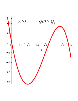
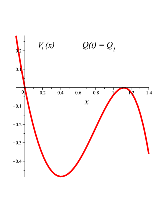
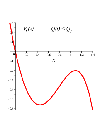
Figure 6. The graph of $V_{t}$ for $Q(t)<Q_{1},Q(t)=Q_{1},Q(t)>Q_{1}$, $Q_{1}\simeq 22.5$

Lemma 4.10.

For $t>0$ $V_{t}(x)$ has negative slope at $x=0$, and it has a unique local maximum at $x=\mathfrak{x}_{t}$ when $x$ positive. Moreover, we have that

(4.50) $$\frac{d}{dt}\mathfrak{x}_{t}<0;\qquad\frac{d}{dt}V_{t}(\mathfrak{x}_{t})<0\qquad\qquad\hbox{ for all }t,$$

and $V_{t}(\mathfrak{x}_{t})<0$ if $Q(t)\in(-28,-26]$. Furthermore, for all $t$ either $x(t)<\mathfrak{x}_{t}$ or $x(t)\geq\mathfrak{x}_{t}$ and $x^{\prime}(t)<0$.

Proof.  Recalling that $K$ satisfies $\frac{d}{dt}K(t)=-4x(t)K(t)$, see (4.20), we have that

$$K(t)=K(0)e^{-4\int_{0}^{t}x(s)ds}.$$

Since $K(0)=4+\alpha^{2}$, $K(t)$ stays positive for every $t$, $Q(t)$ decreases to its limit value $\Lambda_{\varepsilon}\in(-28,-26]$ monotonically in $t$. In particular we have that

$$\frac{\partial}{\partial x}V_{t}(x)|_{x=0}<0\qquad\quad\hbox{ for }t>0.$$

The uniqueness of a local maximum in $x$ for $x>0$ follows from elementary calculus, as well as the fact that $V_{t}(\mathfrak{x}_{t})<0$ if $Q(t)\in(-28,-26]$ and that $\mathfrak{x}_{t}\geq 1$ for all $t>0$. The value $\mathfrak{x}_{t}$ is defined by the equation

$$-Q(t)-60\mathfrak{x}_{t}+32\mathfrak{x}_{t}^{3}=0.$$

Differentiating with respect to $t$ we obtain

$$\left(96\mathfrak{x}_{t}^{2}-60\right)\frac{d}{dt}{\mathfrak{x}}_{t}=\frac{d}{dt}Q(t).$$

The coefficient of $\frac{d}{dt}\mathfrak{x}_{t}$ in the latter formula is positive by the fact that $\mathfrak{x}_{t}\geq 1$, and therefore from $\frac{d}{dt}Q(t)<0$ and from some elementary computations we obtain (4.50).

It remains to prove the last statement. Suppose by contradiction that there exists a first $t_{0}$ for which

(4.51) $$x(t_{0})\geq\mathfrak{x}_{t_{0}};\qquad\qquad x^{\prime}(t_{0})\geq 0.$$

¿From (4.49), from the fact that $Q(t)$ is decreasing and from the fact that $V_{t}(x)$ has no critical points for $x\geq\mathfrak{x}_{t_{0}}$, we deduce that there exists a fixed $\alpha>0$ such that

$$x^{\prime\prime}(t)\geq\alpha(x(t)-\mathfrak{x}_{t_{0}})^{3}\qquad\quad\hbox{ if }x(t)\geq\mathfrak{x}_{t_{0}}.$$

Using the condition (4.51) and some comparison arguments we would then obtain blow-up of $x(t)$ in finite time, which is a contradiction to the fact that $\varepsilon\in(0,\overline{\varepsilon})$.  

We next derive some uniform bounds on $X^{\varepsilon}(t)$, together with some useful consequences.

Lemma 4.11.

There exists a fixed constant $C_{0}>0$ such that $\|X^{\varepsilon}(t)\|\leq C_{0}$ for all $\varepsilon\in(0,\overline{\varepsilon})$ and for all $t>0$.

Proof.  We prove first uniform bounds on $x(t)$. We know that $x(0)=0$, so if $x(t)$ becomes large positive or large negative the function $\mathcal{G}$ becomes large positive (either $x(t)$ is large positive and $x^{\prime}(t)>0$ for some $t$, or $x(t)$ is large negative and $x^{\prime}(t)=0$ for some $t$: for the latter case, recall that $\varepsilon\in(0,\overline{\varepsilon})$, and hence $x(t)$ becomes eventually positive) and has to blow-up in finite time (see Lemma 4.8). This shows uniform bounds on $x(t)$.

Once we have uniform bounds in $x$ we also get uniform bounds in $y=x^{\prime}$ from those on $\mathcal{G}$. By Lemma 4.8 we have that $\mathcal{G}^{\prime}$ stays uniformly bounded, which implies that also $z=y^{\prime}=x^{\prime\prime}$ has to stay uniformly bounded. Then, using (4.14), we also get uniform bounds on $x^{\prime\prime\prime}$, as required. This concludes the proof.  

Corollary 4.12.

There exist $\delta_{1},\delta_{2}>0$ such that

$$\frac{d}{dt}Q(t)<-\delta_{1}<0\qquad\quad\hbox{ for all }t\in[0,\delta_{2}]\hbox{ and for all }\varepsilon\in(0,\overline{\varepsilon}).$$

Moreover $\frac{d^{2}}{dt^{2}}Q(t)$ is uniformly bounded for all $t\geq 0$ and for all $\varepsilon\in(0,\overline{\varepsilon})$.

Proof.  The first statement simply follows from the fact that $\frac{d}{dt}Q(t)=-6K(t)$, that $K(0)=4+\alpha^{2}$, the continuity of $K(t)$ and from Lemma 4.11. The second statement is immediately deduced from $\frac{d^{2}}{dt^{2}}Q(t)=-6K^{\prime}(t)=24xK$ and also from Lemma 4.11.  

We next analyze the behavior of solutions when $x(t)$ attains some small positive value.

Lemma 4.13.

There exist $\delta_{3},\delta_{4}>0$ small and $T_{0}>0$, both independent of $\varepsilon$, such that if $x^{\varepsilon}(\overline{t})=\delta_{3}$ then either

$$\delta_{3}<x^{\varepsilon}(s)\leq 3\qquad\hbox{ for all }s>\overline{t},$$

or

$$\hbox{ there exists }s\in[\overline{t}+\delta_{4},\overline{t}+T_{0}]\hbox{ such that }x^{\varepsilon}(s)=\delta_{3}.$$

Proof.  First, we show that there exist $T_{1}>0$ large and $\delta_{3}>0$ small such that we have the following implication

(4.52) $$\left\{\begin{array}[]{ll}t_{1}<t_{2};&\\ x(t_{1})=x(t_{2})=\delta_{3};&\\ x(t)\geq\delta_{3}\hbox{ for }t\in[t_{1},t_{2}]&\end{array}\right.\qquad\qquad\Rightarrow\qquad\qquad|t_{1}-t_{2}|\leq T_{1}.$$

In fact, suppose that $x(t)\geq\delta_{3}$ on $[t_{1},t_{2}]$. Since $\frac{d}{dt}K(t)=-4xK$, it means that $K$ shrinks exponentially fast for $t\in[t_{1},t_{2}]$. Hence, since $K$ is uniformly bounded (and in particular for $t=t_{1}$) it will get close to zero if $|t_{1}-t_{2}|$ becomes large. Now notice that

(4.53) $$\frac{1}{6}K=\frac{2}{3}+\frac{1}{2}y^{2}+V_{t}(x)$$

and that, by Corollary 4.12, $V_{t}$ at $x=0$ has negative slope (in fact, bounded away from zero for $t\geq t_{1}$). Therefore by $\frac{1}{2}y^{2}+V_{t}(x)\simeq-\frac{2}{3}$, following from (4.53) and the fact that $K$ is small, we deduce that $x(t_{2})$ cannot approach zero if $K$ is close to zero. This implies then (4.52) for $\delta_{3}$ small enough.

Let us now prove the statement of the lemma, assuming by contradiction that none of the two alternatives holds. Let us first suppose that also $x^{\prime}(\overline{t})\geq 0$. By (4.49) and by Corollary 4.12 we have that $x^{\prime}(s)>0$ and $x^{\prime\prime}(s)>\delta_{5}>0$ for $s$ in a right neighborhood of $\overline{t}$ (of size independent of $\varepsilon$). Therefore, by Lemma 4.11 (in particular by the bounds on $z$) $x(s)>\delta_{3}$ for $s\in(\overline{t},\overline{t}+\delta_{4})$ if $\delta_{3},\delta_{4}$ are sufficiently small. Since we are disclaiming the first alternative of the lemma, there will be a first $\tilde{t}>\overline{t}$ for which again $x(\tilde{t})=\delta_{3}$. But then we can apply (4.52) to see that we are in the second alternative.

Suppose now that $x^{\prime}(\overline{t})<0$. By Corollary 4.12 we have that $\frac{d}{dx}V_{t}(x)$ is negative and bounded away from zero for $x(t)\leq\delta_{3}$ and for $t>1$. By (4.49), this means that $x^{\prime\prime}(s)\geq\delta_{6}>0$ for $s>\overline{t}$, as long as $x(s)\leq\delta_{3}$. Therefore (also using the a-priori bounds in Lemma 4.11), we will find $T_{2}>0$ fixed and $\hat{t}\in(\overline{t},\overline{t}+T_{2})$ such that $x(\hat{t})=\delta_{3}$ and for which $x^{\prime}(\hat{t})=\delta_{7}>0$, so we end up in the previous situation ($x^{\prime}(\overline{t})>0$).  

Proof of Proposition 4.9. By Lemma 4.13, (taking $\delta=\delta_{3}$ small), the only case we have to exclude is when $x$ equals $\delta$ along a sequence $\{t_{n}\}$, for which $\delta\leq t_{n+1}-t_{n}\leq T_{0}$. In this case we must have that (see the monotonicity properties in Lemma 4.10)

$$\lim_{t\to+\infty}V_{t}(\mathfrak{x}_{t})\geq-\delta^{2}$$

($\delta$ is taken small), otherwise by (4.49) we would deduce blow-up in finite time (by arguments similar to the proof of Lemma 4.7).

This means that $Q(t)$ (which is monotone decreasing) stays close to some value $Q_{1}>26$ (again, we are using the smallness of $\delta$ and Lemma 4.10) on a sequence of intervals $I_{n}$ of the variable $t$ such that $|I_{n}|\to+\infty$. By Corollary 4.12, we must also have that $\frac{d}{dt}Q(t)$ is small on a sequence of intervals $\tilde{I}_{n}$ with $|\tilde{I}_{n}|\to+\infty$, which means (recall the relation $\frac{d}{dt}Q(t)=-6K(t)$) that $K$ stays close to zero on the sequence of intervals $\tilde{I}_{n}$. But this implies that the function

$$\frac{1}{2}y^{2}+V_{t}(x),$$

the Hamiltonian energy of the trajectory, is negative for $t\in\tilde{I}_{n}$ (see (4.53)), so $x(t)$ cannot reach $\delta$ for $t\in\tilde{I}_{n}$. This concludes the proof.  

We can now prove the main result of this section.

Proposition 4.14.

The solution $X^{\overline{\varepsilon}}$ is globally defined and satisfies condition (4.4), therefore it is geometrically admissible.

Proof.  We begin by proving the following claim

(4.54) $$\Lambda_{\varepsilon}\hbox{ is continuous in }\varepsilon\hbox{ if }\Lambda_{\varepsilon}\in(-28,-26].$$

To see this, let us consider $\varepsilon$ such that $\Lambda_{\varepsilon}\in(-28,-26]$, and choose $\delta>0$ such that $28+\Lambda_{\varepsilon}>200\,\delta>0$. Let us fix a value of $t$ for which $K(t)<\delta$ and $Q(t)-\Lambda_{\varepsilon}<\delta$. ¿From (4.42) and the subsequent arguments one can check that the function $W$ is negative at $t$, and hence $x(t)$ is positive and bounded away from zero (independently of $\varepsilon$ and $\delta$ and the times subsequence to $t$).

Choosing now $\tilde{\varepsilon}$ for which

$$|K^{\varepsilon}(t)-K^{\tilde{\varepsilon}}(t)|<\delta^{2};\qquad\qquad|Q^{\varepsilon}(t)-Q^{\tilde{\varepsilon}}(t)|<\delta^{2},$$

and using (4.20), (4.22) together with the bounds on $x(t)$ we get

$$\frac{d}{dt}\left|K^{\tilde{\varepsilon}}(t)-Q^{\tilde{\varepsilon}}(t)\right|\leq 200K^{\tilde{\varepsilon}}(t),$$

which implies, by integration from $t$ to $\infty$, that

$$\lim_{s\to+\infty}\left|K^{\tilde{\varepsilon}}(s)-Q^{\tilde{\varepsilon}}(s)\right|=\left|K^{\tilde{\varepsilon}}(t)-Q^{\tilde{\varepsilon}}(t)\right|+O(\delta).$$

By our choice of $t$ and $\tilde{\varepsilon}$ then it follows that

$$|\Lambda_{\varepsilon}-\Lambda_{\tilde{\varepsilon}}|\leq O(\delta),$$

which implies the continuity of $\Lambda_{\varepsilon}$.

We show next that

(4.55) $$\lim_{\varepsilon\nearrow\overline{\varepsilon}}\Lambda_{\varepsilon}=-28.$$

This follows from the fact that the sets $\Omega_{\eta,B}$ defined in (4.43) are positively invariant in $t$. In fact, suppose that there exist a sequence $\varepsilon_{n}\nearrow\overline{\varepsilon}$ and a fixed $\delta>0$ such that $\Lambda_{\varepsilon_{n}}\geq-28+\delta$.

By Proposition 4.9 we deduce uniform (in $\varepsilon_{n}$) exponential decay of $K(t)$ and of $Q(t)-\Lambda_{\varepsilon_{n}}$. This means that we can find $T>0$ large, $\eta>0$ small and $B>0$ large such that $X^{\varepsilon_{n}}(T)\in\Omega_{\eta/2,2B}$ for every $n$. But then, by continuity with respect to the initial data, we an also find $\tilde{\varepsilon}>0$ fixed such that $X^{\varepsilon}\in\Omega_{\eta,B}$ for $|\varepsilon-\varepsilon_{n}|\leq\tilde{\varepsilon}$. ¿From the positive invariance of $\Omega_{\eta,B}$ then we reach a contradiction to the definition of $\overline{\varepsilon}$.

Having (4.55), we can now prove the admissibility conditions (4.4). By Proposition 4.9 we know that, if global existence holds, we have uniform exponential convergence to one of the periodic orbits (by (4.20) and (4.22) $K$ and $Q$ converge exponentially to their limit values uniformly in $\varepsilon\in(0,\overline{\varepsilon})$). When $\Lambda_{\varepsilon}$ approaches $-28$, these periodic orbits have longer and longer period, and shadow the homoclinic orbit $X_{0}$ (see the proof of Proposition 4.3). This means that $x(t)$ will be close to $1$ for larger and larger intervals of the parameter $t$, implying

$$\lim_{t\to+\infty}x_{\overline{\alpha}}(t)=1.$$

Therefore our solution is admissible (see Figure 7).  

Figure 7. A numerical plot of the admissible solution $X^{\overline{\varepsilon}}$

5. The case of general coefficients

In this section we consider general determinant functionals of the form

(5.1) $$F_{A}[w]=\gamma_{1}I[w]+\gamma_{2}II[w]+\gamma_{3}III[w].$$

For convenience we set

(5.2) $$\beta=\frac{\gamma_{2}}{12\gamma_{3}}.$$

Our goal is to analyze how the arguments in Sections 3 and 4 may be modified as $\beta$ varies (notice that on locally conformally flat spaces the term $I[w]$ vanishes identically). We are interested in negative values of $\beta$, since it is for these that $\gamma_{2}$ and $\gamma_{3}$ have competing effects. To avoid repetitions, we do not state explicit results but only limit ourselves to a discussion of the proofs.

5.1. The zero U-curvature case

If we study the counterpart of (3.1) with a general choice of the coefficients $\gamma_{i}$’s in $\mathbb{R}^{4}$ and work on the cylinder $\mathfrak{C}=\mathbb{R}\times S^{3}$, (3.3) becomes

(5.3) $$(1+\beta)u^{\prime\prime\prime\prime}-6(u^{\prime})^{2}u^{\prime\prime}+(2-4\beta)u^{\prime\prime}=0.$$

When $\beta=-1$ the only solution is $u^{\prime}=\frac{1}{3}(1-2\beta)$, so from now on we assume that $\beta\neq-1$. The case $\mathcal{C}<0$ is similar to $\mathcal{C}>0$, as one can replace $v$ by $-v$.

Integrating (5.3) and setting $v=u^{\prime}$ we arrive to

$$v^{\prime\prime}=-V_{\mathcal{C},\beta}^{\prime}(v),$$

where

$$V_{\mathcal{C},\beta}(v)=-\frac{1}{2(1+\beta)}v^{4}+\frac{1-2\beta}{1+\beta}v^{2}-\frac{\mathcal{C}}{9}v+\frac{2}{3}.$$

When $\beta<-1$, the potential $V_{\mathcal{C},\beta}$ is coercive, and periodic solutions always exist. For $\mathcal{C}=0$ there are two periodic families of solutions with $v>0$ and $v<0$ respectively, two solutions homoclinic to zero (giving rise to an asymptotically cylindrical metric), and one family of periodic changing-sign solutions.

Letting

$$\mathcal{C}_{\beta}=-\frac{12(1-2\beta)}{1+\beta}\sqrt{\frac{1-2\beta}{3}},$$

a similar qualitative picture, but with a broken symmetry, will persists if $\mathcal{C}\in(0,\mathcal{C}_{\beta})$ (notice that $\mathcal{C}_{\beta}>0$ if $\beta<-1$). For $\mathcal{C}=\mathcal{C}_{\beta}$ only one homoclinic solution will exist, while there will be none for $\mathcal{C}>\mathcal{C}_{\beta}$.

We consider next the case $\beta>-1$. When $\mathcal{C}=0$ we obtain a one-parameter family of Delaunay type solutions as in Proposition 3.1 as well as one heteroclinic solution as in Remark 3.2. When $\mathcal{C}\in(0,-\mathcal{C}_{\beta})$ (notice that now $\mathcal{C}_{\beta}<0$), the heteroclinic solution is replaced by a homoclinic solution, while when $\mathcal{C}=-\mathcal{C}_{\beta}$ only two constant solutions persist.

5.2. The positive U-curvature case

The Euler equation in this case is given by

(5.4) $$(1+\beta)u^{\prime\prime\prime\prime}-6u^{\prime\prime}(u^{\prime})^{2}+(2-4\beta)u^{\prime\prime}=ce^{4u},$$

where the value of $c$ depends on the normalization of $u$.

Imposing evenness in $t$ and requiring the conditions in (4.4) (meaning the we can lift to a solution on $S^{4}$) we find

(5.5) $$c=6\beta,$$

so the ODE under interest is

(5.6) $$(1+\beta)u^{\prime\prime\prime\prime}-6u^{\prime\prime}(u^{\prime})^{2}+(2-4\beta)u^{\prime\prime}=6\beta e^{4u},$$

and the integrated version is

(5.7) $$(1+\beta)u^{\prime\prime\prime}-2(u^{\prime})^{3}+(2-4\beta)u^{\prime}=6\beta\int_{0}^{t}e^{4u}.$$

For the conformal Laplacian $\beta=1/2$, and the round metric is known to be the unique even solution. We discuss some features of the values of $\beta$ smaller than $1/2$, since for $\beta=-7/16$ (corresponding to the determinant of the Paneitz operator), a second solution exists.

We can now follow the same procedure of reducing the ODE to a third-order system. The counterpart of (4.5) is

(5.8) $$-\frac{1}{2}(1+\beta)[u^{\prime\prime}(0)]^{2}=-\left(2\beta+\frac{1}{2}\right)+\frac{3}{2}\beta e^{4u(0)},$$

giving the equation

(5.9) $$\begin{split}\frac{1}{4}(1+\beta)u^{\prime\prime\prime\prime}&-(1+\beta)u^{\prime\prime\prime}u^{\prime}+\frac{1}{2}(1+\beta)(u^{\prime\prime})^{2}-\frac{3}{2}u^{\prime\prime}(u^{\prime})^{2}\\ &+\frac{1}{4}(2-4\beta)u^{\prime\prime}+\frac{3}{2}(u^{\prime})^{4}+(2\beta-1)(u^{\prime})^{2}-\left(2\beta+\frac{1}{2}\right)=0.\end{split}$$

As before, let $x=-u^{\prime}$, $y=x^{\prime}$, $z=y^{\prime}$, we end up with the system

(5.10) $$\begin{split}x^{\prime}&=y,\\ y^{\prime}&=z,\\ z^{\prime}&=-4xz+\frac{6}{1+\beta}x^{2}y+2y^{2}+2\left(\frac{2\beta-1}{1+\beta}\right)y\\ &+\frac{6}{1+\beta}x^{4}+4\left(\frac{2\beta-1}{1+\beta}\right)x^{2}-2\left(\frac{4\beta+1}{1+\beta}\right),\end{split}$$

with initial conditions

(5.11) $$\begin{split}x(0)&=0,\\ y(0)&=-u^{\prime\prime}(0)>0,\\ z(0)&=0.\end{split}$$

For general $\beta$, we define $K_{\beta}$ and $Q_{\beta}$ by

(5.12) $$K_{\beta}=-6xz+3y^{2}+\frac{9}{1+\beta}x^{4}-6\frac{(1-2\beta)}{(1+\beta)}x^{2}-3\frac{(1+4\beta)}{(1+\beta)},$$

(5.13) $$Q_{\beta}=-16(1+\beta)z+32x^{3}+32(2\beta-1)x.$$

Then along solutions of (5.10) one finds

(5.14) $$\frac{dK_{\beta}}{dt}=-4xK_{\beta},$$

(5.15) $$\frac{dQ_{\beta}}{dt}=-\frac{32}{3}(1+\beta)K_{\beta}.$$

Repeating the arguments in the previous subsection one can see that the limit values of $K_{\beta}$ and $Q_{\beta}$ for an admissible solution are $0$ and $64\beta$ respectively. The counterpart of (4.49) is

$$x^{\prime\prime}=\frac{1}{1+\beta}\left[2x^{3}+2(2\beta-1)x-4\beta\right],$$

namely a Newton equation with potential

$$V_{t,\beta}(x):=\frac{Q_{\beta}(t)}{16(1+\beta)}x-\frac{1}{2(1+\beta)}x^{4}-\frac{2\beta-1}{1+\beta}x^{2}.$$

In the limit $t\to+\infty$, namely when $Q_{\beta}(t)$ tends to $64\beta$, $V_{t,\beta}$ attains a negative maximum at some positive $x$ if and only if $-1<\beta<-\frac{1}{4}$. For these values of $\beta$ then, the above argument can be repeated with minor changes to get existence of a second solution. Notice that this applies to the half-torsion case, for which $\beta=-\frac{31}{58}$.

For $\beta=-1$, $Q_{\beta}$ has the wrong monotonicity by (5.15), while $\lim_{t\to+\infty}V_{t,\beta}$ has a qualitatively different profile. For $\beta>-\frac{1}{4}$ instead, the uniform estimates in Proposition 4.9 break down. A numerical simulation indeed indicates that, although the counterpart of Proposition 4.6 holds, $X^{\overline{\varepsilon}}$ is not admissible.

References

- [AAR] Pierre Albin, Clara L. Aldana, and Frederic Rochon, Ricci flow and the determinant of the laplacian on non-compact surfaces, preprint, 2009. http://arxiv.org/abs/0909.0807.
- [Ada88] David R. Adams, A sharp inequality of J. Moser for higher order derivatives, Ann. of Math. (2) 128 (1988), no. 2, 385–398.
- [AS64] Milton Abramowitz and Irene A. Stegun, Handbook of mathematical functions with formulas, graphs, and mathematical tables, National Bureau of Standards Applied Mathematics Series, vol. 55, For sale by the Superintendent of Documents, U.S. Government Printing Office, Washington, D.C., 1964.
- [BCY92] Thomas P. Branson, Sun-Yung A. Chang, and Paul C. Yang, Estimates and extremals for zeta function determinants on four-manifolds, Comm. Math. Phys. 149 (1992), no. 2, 241–262. MR 1186028 (93m:58116)
- [BM] Dmitriy M. Belov and Gregory W. Moore, Holographic action for the self-dual field, preprint, 2006. http://arxiv.org/abs/hep-th/0605038v1.
- [BN83] Haim Brézis and Louis Nirenberg, Positive solutions of nonlinear elliptic equations involving critical Sobolev exponents, Comm. Pure Appl. Math. 36 (1983), no. 4, 437–477.
- [BO91] Thomas P. Branson and Bent rsted, Explicit functional determinants in four dimensions, Proc. Amer. Math. Soc. 113 (1991), no. 3, 669–682.
- [Bra96] Thomas P. Branson, An anomaly associated with 4-dimensional quantum gravity, Comm. Math. Phys. 178 (1996), 301–309.
- [CGY99] Sun-Yung A. Chang, Matthew J. Gursky, and Paul C. Yang, Regularity of a fourth order nonlinear PDE with critical exponent, Amer. J. Math. 121 (1999), no. 2, 215–257.
- [Con94] Alain Connes, Noncommutative geometry, Academic Press, San Diego, CA, 1994.
- [CY95] Sun-Yung A. Chang and Paul C. Yang, Extremal metrics of zeta function determinants on -manifolds, Ann. of Math. (2) 142 (1995), no. 1, 171–212.
- [DM08] Zindine Djadli and Andrea Malchiodi, Existence of conformal metrics with constant -curvature, Ann. of Math. (2) 168 (2008), no. 3, 813–858.
- [GOAR08] Hans-Christoph Grunau, Mohameden Ould Ahmedou, and Wolfgang Reichel, The Paneitz equation in hyperbolic space, Ann. Inst. H. Poincaré Anal. Non Linéaire 25 (2008), no. 5, 847–864. MR 2457814 (2009h:58076)
- [Gur97] Matthew J. Gursky, Uniqueness of the functional determinant, Comm. Math. Phys. 189 (1997), no. 3, 655–665.
- [Gur99] by same author, The principal eigenvalue of a conformally invariant differential operator, with an application to semilinear elliptic PDE, Comm. Math. Phys. 207 (1999), no. 1, 131–143.
- [Juh09] Andreas Juhl, Families of conformally covariant differential operators, -curvature and holography, Progress in Mathematics, vol. 275, Birkhäuser Verlag, Basel, 2009.
- [Mon] Samuel Monnier, Geometric quantization and the metric dependence of the self-dual field theory, preprint, 2010. http://arxiv.org/abs/1011.5890v2.
- [OPS88a] B. Osgood, R. Phillips, and P. Sarnak, Compact isospectral sets of surfaces, J. Funct. Anal. 80 (1988), no. 1, 212–234.
- [OPS88b] by same author, Extremals of determinants of laplacians, J. Funct. Anal. 80 (1988), no. 1, 148–211.
- [Pol81] Alexander M. Polyakov, Quantum geometry of fermionic strings, Phys. Lett. B 103 (1981), no. 3, 211–213.
- [RS71] D. B. Ray and I. M. Singer, -torsion and the Laplacian on Riemannian manifolds, Advances in Math. 7 (1971), 145–210. MR 0295381 (45 #4447)
- [UV00] Karen K. Uhlenbeck and Jeff A. Viaclovsky, Regularity of weak solutions to critical exponent variational equations, Math. Res. Lett. 7 (2000), no. 5-6, 651–656.
- [Via00] Jeff A. Viaclovsky, Conformal geometry, contact geometry, and the calculus of variations, Duke Math. J. 101 (2000), 283–316.
- [Wit97] Edward Witten, Five-brane effective action in M-theory, J. Geom. Phys. 22 (1997), 103–133.