CANDELS: The Cosmic Assembly Near-infrared Deep Extragalactic Legacy Survey

Abstract

The Cosmic Assembly Near-infrared Deep Extragalactic Legacy Survey (CANDELS) is designed to document the first third of galactic evolution, over the approximate redshift ($z$) range 8–1.5. It will image $>$250,000 distant galaxies using three separate cameras on the Hubble Space Telescope, from the mid-ultraviolet to the near-infrared, and will find and measure Type Ia supernovae at $z>1.5$ to test their accuracy as standardizable candles for cosmology. Five premier multi-wavelength sky regions are selected, each with extensive ancillary data. The use of five widely separated fields mitigates cosmic variance and yields statistically robust and complete samples of galaxies down to a stellar mass of $10^{9}{\rm M}_{\odot}$ to $z\approx 2$, reaching the knee of the ultraviolet luminosity function (UVLF) of galaxies to $z\approx 8$. The survey covers approximately 800 arcmin² and is divided into two parts. The CANDELS/Deep survey ($5\sigma$ point-source limit $H=27.7\,$mag) covers $\sim 125$ arcmin² within GOODS-N and GOODS-S. The CANDELS/Wide survey includes GOODS and three additional fields (EGS, COSMOS, and UDS) and covers the full area to a $5\sigma$ point-source limit of $H\gtrsim 27.0$ mag. Together with the Hubble Ultra Deep Fields, the strategy creates a three-tiered “wedding cake” approach that has proven efficient for extragalactic surveys. Data from the survey are nonproprietary and are useful for a wide variety of science investigations. In this paper, we describe the basic motivations for the survey, the CANDELS team science goals and the resulting observational requirements, the field selection and geometry, and the observing design. The Hubble data processing and products are described in a companion paper.

1. Introduction

During the past decade, the Hubble Space Telescope (HST) and other telescopes have fueled a series of remarkable discoveries in cosmology that would have seemed impossible only a few short years ago. Galaxies are now routinely found when the Universe was only 5% of its current age and before 99% of present-day stars had formed. Distant Type Ia supernovae (SNe Ia) showed that the expansion of the Universe was decelerating for the first $\sim 9$ Gyr, followed by acceleration due to a mysterious “dark energy” whose nature remains completely unknown. The troika of Hubble, Spitzer, and Chandra revealed a complex interplay between galaxy mergers, star formation, and black holes over cosmic time that spawned the new concept of galaxy/black hole “co-evolution.”

This rapid progress can be attributed in part to an unprecedented degree of coordination between observatories across the electromagnetic spectrum in which a few small regions of sky were observed as deeply as possible at all accessible wavelengths. Such regions have become “magnet” regions whose total scientific value now far exceeds that of their individual surveys.

The Great Observatories Origins Deep Survey (GOODS; Giavalisco et al. 2004) possesses the deepest data on the sky from virtually every telescope: Hubble, Spitzer, Chandra, Herschel, the VLA, and many other observatories both in space and on the ground. However, the GOODS-North and GOODS-South fields together subtend only about 300 arcmin², which makes them too small for science goals involving rare and/or massive objects. Samples are limited, and count fluctuations tend to be large owing to the high intrinsic bias and cosmic variance of massive halos. GOODS HST images furthermore probe only optical wavelengths, which are strongly biased toward ongoing star-forming regions and miss the older stars beyond redshift $z\approx 1.3$.

With a survey speed gain of a factor of $\sim 30$ over NICMOS for galaxy imaging, the new WFC3/IR (infrared) camera enables much more ambitious near-IR surveys than were previously possible with Hubble. For example, the single-filter GOODS NICMOS Survey (GNS; Conselice et al. 2011a) required 180 HST orbits to survey 45 arcmin² to a limiting magnitude of $H_{\rm AB}\approx 26.5$. By comparison, WFC3/IR enables a two-filter survey of five times the GNS area to limiting magnitudes of $H_{\rm AB}\gtrsim 27.1$ and $J_{\rm AB}\gtrsim 27.0$ — using half the orbits required for the GNS. The capacity for longer-wavelength and larger-area surveys now allows Hubble to: follow galaxies well into the reionization era; measure spectra and light curves for SNe Ia in the deceleration era; and measure rest-frame optical shapes and sizes of galaxies at a time ($z\approx 2$) when cosmic luminosity peaked for both star formation and active galactic nuclei (AGNs), and when the Hubble sequence was starting to take shape. The power of WFC3/IR imaging for distant galaxies is demonstrated in Figure 1, which compares GOODS-depth 4-orbit F775W images from the Hubble Advanced Camera for Surveys (ACS) with 2-orbit images from WFC3/IR. Regions with red colors due to heavy dust or old stars leap out with the WFC3/IR, in many cases leading to a new interpretation of the object.

Figure 1.— Four-orbit images of HUDF galaxies from ACS vs. 2-orbit images from WFC3/IR illustrate the importance of WFC3/IR for studying distant galaxy structure. WFC3/IR unveils the true stellar mass distributions of these galaxies unbiased by young stars and obscuring dust. The new structures that emerge in many cases inspire revised interpretations of these objects, as indicated.

Given the power of this gain, there is strong motivation to extend deep-field WFC3/IR imaging beyond the GOODS regions to larger areas. Three well-studied regions in the sky are natural candidates for this extension: COSMOS (Scoville et al. 2007), the Extended Groth Strip (EGS; Davis et al. 2007), and the UKIDSS Ultra-deep Survey field (UDS; Lawrence et al. 2007; Cirasuolo et al. 2007). These fields are larger than GOODS and already have high-quality (though generally shallower) multi-wavelength data. Establishing multiple, statistically independent WFC3/IR regions over the sky would also minimize cosmic variance and facilitate follow-up observations by ground-based telescopes.

Several teams responded to the Hubble Multi-Cycle Treasury Program Call for Proposals with programs targeting high-latitude fields using WFC3/IR to study galaxy evolution. Two teams targeted the above five fields and also proposed to find high-redshift SNe Ia to improve constraints on cosmic deceleration and acceleration. The program led by Ferguson proposed to observe the full 300 arcmin² of the GOODS fields to uniform depth in $YJH$. This proposal contained time for both spectroscopic and photometric SN Ia follow-up observations and took advantage of GOODS-N in the Hubble Continuous Viewing Zone (CVZ) to obtain far-ultraviolet (UV) images on the day side of the orbit when the sky is too bright for broadband IR imaging. The second program, led by Faber, proposed imaging half the area of the two GOODS fields to about twice the depth of the Ferguson program and also added shallower imaging over $\sim 1000$ arcmin² in EGS, COSMOS, UDS, and the Extended Chandra Deep Field South. ACS parallels were included to broaden total wavelength coverage, deepen existing ACS mosaics, and add a new ACS mosaic in UDS, where none existed. SN Ia searches were also included, but the proposal did not contain time for SN follow-up observations, nor did it feature UV imaging.

The Hubble time-allocation committee (TAC) saw merit in both proposals and charged the two teams to craft a joint program to retain the best features of both programs yet fit within 902 orbits. This was challenging, owing to four requirements mandated by the TAC: (1) visit all WFC3/IR tiles at least twice with the proper cadence for finding SNe Ia ($\sim 60$ days; this severely restricts the range of allowable dates and ORIENTs in each field), (2) discriminate SNe Ia candidates from other interlopers (requires very specific multi-wavelength data at each visit), (3) put as many ACS parallels as possible on top of each WFC3/IR tile (further restricting Hubble observation dates and ORIENTs), and (4) maximize the overlap of Hubble data on top of existing ancillary data (compatible dates and ORIENTs become vanishingly small). Further complicating matters, the Hubble TAC also approved the CLASH program on clusters of galaxies by Postman et al. (GO 12065), including SN discovery and follow-up observations, with the mandate that it be coordinated with the SN Ia program here. The SN portions of both proposals were consolidated under a separate program by Riess et al. (GO 12099), and the SN Ia follow-up orbits from both programs were pooled. Our program takes prime responsibility for the highest-redshift SNe ($z>1.3$), while CLASH addresses SNe at lower redshifts.

The resulting observing program, now entitled the Cosmic Assembly Near-infrared Extragalactic Legacy Survey (CANDELS), targets five distinct fields (GOODS-N, GOODS-S, EGS, UDS, and COSMOS) at two distinct depths. Henceforth, we will refer to the deep portion of the survey as “CANDELS/Deep” and the shallow portion as “CANDELS/Wide.” Adding in the Hubble Ultra Deep Fields (HUDF) makes a three-tiered “wedding cake” approach, which has proven to be very effective with extragalactic surveys. CANDELS/Wide has exposures in all five CANDELS fields, while CANDELS/Deep is only in GOODS-S and GOODS-N.

The outline of this paper is as follows. We first provide a brief synopsis of the survey in §2. We follow in §3 with a detailed description of the major science goals along with their corresponding observational requirements that CANDELS addresses. We synthesize the combined observing requirements in §4 with regard to facets of our survey. A description of the particular survey fields and an overview of existing ancillary data are provided in §5. Section 6 describes the detailed observing plan, including the schedule of observations. Section 7 summarizes the paper, along with a brief description of the CANDELS data reduction and data products; a much more complete description is given by Koekemoer et al. (2011), which is intended to be read as a companion paper to this one.

Where needed, we adopt the following cosmological parameters: $H_{0}=70$ km s^-1 Mpc^-1; $\Omega_{\rm tot},\Omega_{\Lambda},\Omega_{\rm m}=1,0.3,0.7$ (respectively), though numbers used in individual calculations may differ slightly from these values. All magnitudes are expressed in the AB system (Oke & Gunn 1983).

2. CANDELS Synopsis

Table 1 provides a convenient summary of the survey, listing the various filters and corresponding total exposure within each field, along with each field’s coordinates and dimensions. The Hubble data are of several different types, including images from WFC3/IR and WFC3/UVIS (both UV and optical) plus extensive ACS parallel exposures. Extra grism and direct images will also be included for SN Ia follow-up observations (see §3.5), but their exposure lengths and locations are not pre-planned. They are not included in Table 1. In perusing the table, it may be useful to look ahead at Figures 5–9, which illustrate the layout of exposures on the sky.

Table 1CANDELS at a glance

Field	Coordinates	Tier	WFC3/IR Tiling	HST Orbits/Tile	IR Filters	UV/Optical Filters
GOODS-N	189.228621, $+$62.238572	Deep	$\sim 3\times 5$	$\sim$13	YJH	UV,UI(WVz)
GOODS-N	189.228621, $+$62.238572	Wide	2 @ $\sim 2\times 4$	$\sim$3	YJH	Iz(W)
GOODS-S	53.122751, $-$27.805089	Deep	$\sim 3\times 5$	$\sim$13	YJH	I(WVz)
GOODS-S	53.122751, $-$27.805089	Wide	$\sim 2\times 4$	$\sim$3	YJH	Iz(W)
COSMOS	150.116321, $+$2.2009731	Wide	$4\times 11$	$\sim$2	JH	VI(W)
EGS	214.825000, $+$52.825000	Wide	$3\times 15$	$\sim$2	JH	VI(W)
UDS	34.406250, $-$5.2000000	Wide	$4\times 11$	$\sim$2	JH	VI(W)

The three purely Wide fields (UDS, COSMOS, and EGS, Figs. 7–9) consist of a contiguous mosaic of overlapping WFC3/IR tiles (shown in blue) along with a contemporaneous mosaic of ACS parallel exposures (shown in magenta). The two cameras are offset by $\sim 6^{\prime}$, but overlap between them is maximized by choosing the appropriate telescope roll angle. The Wide exposures are taken over the course of two HST orbits, with exposure time allocated roughly 2:1 between F160W and F125W. The observations are scheduled in two visits separated by $\sim 52$ days in order to find SNe Ia. The stacked exposure time is effectively twice as long in ACS (i.e., 4 orbits) on account of its larger field of view, and its time is divided roughly 2:1 between F814W and F606W. In the small region where the WFC3/IR lacks ACS parallel overlap, we sacrifice WFC3/IR depth to obtain a short exposure in the WFC3/UVIS “white-light” filter F350LP for SN type discrimination.

The GOODS fields contain both Deep and Wide exposure regions. In addition, GOODS-S also contains the ERS data (Windhorst et al. 2011), which we have taken into account in our planning and include in the CANDELS quoted areas because its filters and exposure times match well to ours (see §6.2). The two GOODS layouts are shown in Figures 5 and 6. The Deep portion of each one is a central region of approximately $3\times 5$ WFC3/IR tiles, which is observed to an effective depth of 3 orbits in F105W and 4 orbits in F125W and F160W. To the north and south lie roughly rectangular “flanking fields” each covered by 8–9 WFC3/IR tiles, which are observed using the Wide strategy of 2 orbits in $J$+$H$. The flanking fields additionally receive an orbit of F105W. The net result is coverage over most of the GOODS fields to at least $\sim 1$-orbit depth in $YJH$, plus deeper coverage in all three filters within the Deep areas.

Executing the GOODS exposures requires $\sim 15$ visits to each field, and virtually all $J$+$H$ orbits are employed in SN Ia searching. The filter layouts at each visit are shown for GOODS-S in Figures 11 and 12 (detailed visits for GOODS-N have not yet been finalized). Because the telescope roll angle cannot be held constant across so many visits, the matching ACS parallel exposures (which are always taken) are distributed around the region in a complicated way. These parallels are taken in F606W, F814W, and F850LP according to a complex scheme explained in §6.2. For now, it is sufficient to note that most of the ACS parallels use F814W, for the purpose of identifying high-$z$ Lyman-break “drop-out” galaxies. Because there is poor overlap between WFC3/IR exposures and their ACS parallels during any given epoch, all GOODS $J$+$H$ orbits include a short WFC3/UVIS F350LP exposure as noted above for CANDELS/Wide. Finally, Table 1 also lists special WFC3/UVIS exposures taken during GOODS-N CVZ opportunities, of total duration $\sim 13$ ks in F275W and $\sim 7$ ks in F336W. Exposure maps of the expected final data in GOODS-S are shown in Figures 17 and 18, including all previous legacy exposures in HST broadband filters (the GOODS-N maps in Figs. 20 and 21 are preliminary).

Realizing the full science potential of this extensive but complex dataset will require closely interfacing with many other ground-based and space-based surveys. Among these we particularly mention SEDS, the Spitzer Warm Mission Extended Deep Survey, whose deep 3.6 $\micron$ and 4.8 $\micron$ data points provide vital stellar masses (the CANDELS fields are completely embedded within the SEDS regions). The total database is rich, far richer than our team can exploit. Because of this, and the Treasury nature of the CANDELS program, we are moving speedily to process and make the Hubble data public (for details, see Koekemoer et al. 2011). The first CANDELS data release occurred on 12 January 2011, 60 days after the first epoch was acquired in GOODS-S. As a further service to the community, we are constructing separate websites for each CANDELS field to collect and serve the ancillary data. For further information, please visit the CANDELS website.

3. Science Goals

The Multi-Cycle Treasury (MCT) Program was established to address high-impact science questions that require Hubble observations on a scale that cannot be accommodated within the standard time-allocation process. MCT programs are also intended to seed a wide variety of compelling scientific investigations. Deep WFC3/IR observations of well-studied fields at high Galactic latitudes naturally meet these two criteria.

In this section we outline the CANDELS science goals, prefixed by a brief discussion in §3.1 of the theoretical tools that are being developed for the CANDELS program. Most of our investigations of galaxies and AGNs divide naturally into two epochs. In §3.2 (“cosmic dawn”), we discuss studies of very early galaxies during the reionization era. In §3.3 (“cosmic high noon”), we discuss the growth and transformation of galaxies during the era of peak star formation and AGN activity. Section 3.4 describes science goals enabled by UV observations that exploit the GOODS-N CVZ. Section 3.5 describes the use of high-$z$ SNe to constrain the dynamics of dark energy, measure the evolution of SN rates, and test whether SNe Ia remain viable as standardizable candles at early epochs. Finally, §3.6 describes science goals enabled by the grism portion of the program. The complete list of goals is collected for reference in Table 2. Work is proceeding within the team on all of these topics.

Table 2CANDELS Primary Scientific Goals

No.	Goal
Cosmic Dawn (CD): Formation and early evolution of galaxies and AGNs
CD1	Improve constraints on the bright end of the galaxy LF at $z\approx 7$ and 8 and make $z\approx 6$ measurements more robust. Combine with WFC3/IR data on fainter magnitudes to constrain the UV luminosity density of the Universe at the end of the reionization era.
CD2	Constrain star-formation rates, ages, metallicities, stellar masses, and dust contents of galaxies at the end of the reionization era, $z\approx 6$–10. Tighten estimates of the evolution of stellar mass, dust and metallicity at $z=4$–8 by combining WFC3 data with very deep Spitzer IRAC photometry.
CD3	Measure fluctuations in the near-IR background light, at sensitivities sufficiently faint and angular scales sufficiently large to constrain reionization models.
CD4	Use clustering statistics to estimate the dark-halo masses of high-redshift galaxies with double the area of prior Hubble surveys.
CD5	Search deep WFC3/IR images for AGN dropout candidates at $z>6$–7 and constrain the AGN LF.
Cosmic High Noon (CN): The peak of star formation and AGN activity
CN1	Conduct a mass-limited census of galaxies down to $M_{*}=2\times 10^{9}$ M⊙ at $z\approx 2$ and determine redshifts, star-formation rates, and stellar masses from broadband spectral-energy distributions (SEDs). Quantify patterns of star formation versus stellar mass and other variables and measure the cosmic-integrated stellar mass and star-formation rates to high accuracy.
CN2	Obtain rest-frame optical morphologies and structural parameters of $z\approx 2$ galaxies, including morphological types, radii, stellar mass surface densities, and quantitative disk, spheroid, and interaction measures. Use these to address the relationship between galactic structure, star-formation history, and mass assembly.
CN3	Detect galaxy sub-structures and measure their stellar masses. Use these data to assess disk instabilities, quantify internal patterns of star formation, and test bulge formation by clump migration to the centers of galaxies.
CN4	Conduct the deepest and most unbiased census yet of active galaxies at $z\gtrsim 2$ selected by X-ray, IR, optical spectra, and optical/NIR variability. Test models for the co-evolution of black holes and galaxies and triggering mechanisms using demographic data on host properties, including morphology and interaction fraction.
Ultraviolet Observations (UV): Hot stars at $1<z<3.5$
UV1	Constrain the Lyman-continuum escape fraction for galaxies at $z\approx 2.5$.
UV2	Identify Lyman-break galaxies at $z\approx 2.5$ and compare their properties to higher-$z$ Lyman-break galaxy samples.
UV3	Estimate the star-formation rate in dwarf galaxies to $z>1$ to test whether dwarf galaxies are “turning on” as the UV background declines at low redshift.
Supernovae (SN): Standardizable candles beyond $z\approx 1$
SN1	Test for the evolution of SNe Ia as distance indicators by observing them at $z>1.5$, where the effects of dark energy are expected to be insignificant but the effects of the evolution of the SN Ia white-dwarf progenitor masses ought to be significant.
SN2	Refine constraints on the time variation of the cosmic equation-of-state parameter, on a path to more than doubling the strength of this crucial test of a cosmological constant by the end of HST’s life.
SN3	Measure the SN Ia rate at $z\approx 2$ to constrain progenitor models by detecting the offset between the peak of the cosmic star-formation rate and the peak of the cosmic rate of SNe Ia.

3.1. Theory Support

Theoretical predictions have been an integral part of the project’s development since its inception. We have extracted merger trees from the new Bolshoi N-body simulation (Klypin et al. 2010), which also track the evolution of sub-halos. We then extract lightcones that mimic the geometry of the CANDELS fields, with many realizations of each field in order to study cosmic variance. These lightcones are populated with galaxies using several methods: (1) Sub-Halo Abundance Matching (SHAM), a variant of Halo Occupation Distribution modeling, in which stellar masses or luminosities are assigned to (sub-)halos such that the observed galaxy abundance is reproduced (Behroozi et al. 2010); (2) semi-analytic models (SAMs), which use simplified recipes to track the main physical processes of galaxy formation. We are using three different, independently developed SAM codes, based on updated versions of the models developed by Somerville et al. (2008b), Croton et al. (2006), and Lu et al. (2010), that are being run in the same Bolshoi-based merger trees. This will allow us to explore the impact of different model assumptions on galaxy observables.

All three SAM models include treatments of radiative cooling of gas, star formation, stellar feedback, and stellar population synthesis. The Somerville and Croton SAMs also include modeling of black hole formation and growth, and so can track AGN activity. We are developing more detailed and accurate modeling of the radial sizes of disks and spheroids in the SAMs, using an approach based on the work of Dutton & van den Bosch (2009) in the case of the former, and using the recipe based on mass ratio, orbit parameters, and gas content taken from merger simulations by Covington et al. (2011) for the latter. Using simple analytic prescriptions for dust extinction, we will use the SAMs to create synthetic images based on these mock catalogs, assuming smooth parameterized light profiles for the galaxies. A set of mock catalogs, containing physical properties such as stellar mass and star-formation rate (SFR), as well as observables such as luminosities in all CANDELS bands, will be released to the public through a queryable database. The synthetic images will also be made publicly available.

In addition, several team members are pursuing N-body and hydrodynamic simulations using a variety of approaches. To complement Bolshoi, Piero Madau is computing Silver River, a higher-resolution version of his previous N-body Via Lactea Milky Way simulation. Romeel Davé is using a proprietary version of Gadget-2 to track gas infall, star formation, and stellar feedback in very high-redshift galaxies (Finlator et al. 2011). Working with multiple teams, Avishai Dekel is guiding the computation of early disky galaxies at $z\approx 2$ with particular reference to clump formation; early results were presented in Ceverino et al. (2010). The simulation efforts make use of a wide range of codes and numerical techniques, including ART, ENZO, RAMSES, GADGET, and GASOLINE. Finally, the theory effort includes postprocessing of hydrodynamic simulations with the SUNRISE radiative transfer code to produce realistic images and spectra, including the effects of absorption and scattering by dust (Jonsson et al. 2010). Our goal is to create a library of $z\gtrsim 2$ galaxy images that can be used to help interpret the CANDELS observations. These images will also be released to the public.

3.2. Galaxies and AGNs: Cosmic Dawn

The science aims of CANDELS for redshifts $z\gtrsim 3$ are collected together under the rubric “cosmic dawn.” Within a few months of installation, WFC3 proved its power for galaxy studies in this era by uncovering a wealth of new objects at $z>6$ (e.g., Bouwens et al. 2010a; McLure et al. 2010; Yan et al. 2010). WFC3/IR can potentially detect objects as distant as $z\gtrsim 10$, for which all bands shortward of F160W drop out (Bouwens et al. 2011a). It also enables proper 3-band color selection of Lyman-break galaxies (LBGs) at $5<z<10$, which ACS would detect in only two, one, or zero filters, and it offers multiple bands for better constraining stellar populations and reddening of galaxies at $3<z<7$.

We describe five science drivers for the cosmic dawn epoch, and summarize them in Table 2.

(CD1) Improve constraints on the bright end of the galaxy luminosity function at $z\approx 7$–8 and make $z\approx 6$ measurements more robust. Combine with WFC3/IR data on fainter magnitudes to constrain the UV luminosity density of the Universe at the end of the reionization era.

Quasi-stellar object (QSO) spectra (Fan et al. 2006) and WMAP polarization (Page et al. 2007; Spergel et al. 2007) both indicate that the intergalactic medium (IGM) was reionized between 0.5 and 1 Gyr after the Big Bang. Moreover, the IGM was seeded with metals to $Z\approx 4\times 10^{-4}$ within the first billion years, and the energy released by the stars that produced these metals appears sufficient to reionize the IGM (Songaila 2001; Ryan-Weber et al. 2006). However, the exact stars emitting this radiation have not yet been identified. The bright end of the UVLF of star-forming galaxies is evolving rapidly at $4<z<7$ (e.g., Dickinson et al. 2004, Bouwens et al. 2007, 2008, 2011b), but the UV flux from these bright galaxies thus far appears insufficient to explain reionization. Estimates of stellar masses and ages at $z=5$–6 also hint that some galaxies may have experienced a rapid burst of star formation in the first Gyr (Yan et al. 2005, 2006; Eyles et al. 2005, 2007; Mobasher et al. 2005; Wiklind et al. 2008), but the connection with reionization is unclear. Finally, the bright end of the UVLF is itself worthy of study, as these bright high-$z$ galaxies are statistically the most likely forerunners of massive galaxies today (Papovich et al. 2011).

The rapid evolution of the UVLF reflects an interplay between the growth of dark matter halos, fueling of star formation, regulation by feedback, and dust obscuration. Empirical constraints on these basic elements of early galaxy growth are essential. CANDELS will provide several fundamental tools needed for this, including measurements of the rest-frame UVLF, the stellar-mass function, the color-luminosity and size-luminosity relations, and the angular correlation function. Many CANDELS galaxies will be bright enough for detailed morphological study and will be detected individually beyond $3\,\,\mu\rm m$ by the Spitzer/SEDS IRAC survey. For others, CANDELS will provide large statistical samples for IRAC stacking.

Table 3Numbers of Representative Objects

Object class	Redshift range	$H\tablenotemark{a}$	Deep+Wide	Deep only
$M_{\rm UV}<-19.0$	6.5–7.5	27.9	$\cdots$	280–480
$M_{\rm UV}<-20.0$	6.5–7.5	26.9	160–240	25–35
$M_{\rm UV}<-21.3$	6.5–7.5	25.6	$\sim 10$	$\sim 1$
$M_{\rm UV}<-19.0$	7.5–8.5	28.1	$\cdots$	120–280
$M_{\rm UV}<-20.0$	7.5–8.5	27.1	70–150	10–20
$M_{\rm UV}<-21.2$	7.5–8.5	25.9	$\sim 10$	$\sim 1$
$M_{*}>10^{9}$M⊙	1.5-2.5	28.0	$\cdots$	1000
$M_{*}>10^{10}$M⊙	1.5-2.5	25.5	3000	450
$M_{*}>10^{11}$M⊙	1.5-2.5	23.0	300	40
$M_{*}>10^{11.6}$M⊙	1.5-2.5	21.5	$\sim$10	$\sim$1
Detailed morphologies, Wide	1.5–2.5	24.0	1200	$\cdots$
Detailed morphologies, Deep	1.5–2.5	24.7	$\cdots$	250
X-ray sources	1.5–2.5	$\cdots$	200	30
Mergers	1.5–2.5	$\cdots$	300	45

Note. — $H$-band magnitude limits for various classes of galaxies, together with the estimated number of objects brighter than this limit within CANDELS.

Nailing down the number of bright galaxies impacts the shape of the LF as a whole, and hence the estimate of total UV density. The distribution of galaxy luminosities is traditionally characterized by the Schechter (1976) function:

$$N(M)dL=\phi^{*}(L/L^{*})^{\alpha}\exp(-L/L^{*})d(L/L^{*}),$$ (1)

which thus far fits distant galaxies fairly well. The goal is to robustly identify samples of high-redshift galaxies and measure the characteristic luminosity $L^{*}$, the space density $\phi^{*}$, and faint-end slope $\alpha$. However, the LF cannot be reliably constrained with galaxies in only a narrow range of sub-$L^{\ast}$ luminosities alone — accurate measurements at the bright end and near the knee are also needed, which CANDELS will provide.

At $z\approx 8$, current LFs are based on small fields with only a handful of objects, most with $L_{\rm UV}\lesssim L^{\ast}$ (there are only $\sim 1.0$ galaxies with $L>L^{\ast}$ per $\Delta z=1$ per WFC3/IR field at $z\geq 6$; see Table 3). The uncertainty in the luminosity density at $L>L^{*}$ prior to the WFC3 era was $\sim 100$%. The population of $z\gtrsim 8$ galaxies now has grown to the low dozens from early Hubble WFC3/IR data (Trenti et al. 2011; Grazian et al. 2011; Yan et al. 2011; Bouwens et al. 2011b; McLure et al. 2011; Oesch et al. 2011) and some heroic efforts from the ground (Ouchi et al. 2009, 2010; Ota et al. 2010; Castellano et al. 2010b; Vanzella et al. 2011); recent results are summarized in Figure 3.2. Nonetheless, it is worth noting that there is no particularly good physical reason to adopt the exponential cutoff at the bright end of the LF given by Equation 1. If one drops this assumption, then estimates of the overall UV luminosity density are as sensitive to the shape of the LF at the bright end as they are to the slope at the faint end.

Collected data on luminosity functions (LFs) of distant LBGs at $z\approx 7$ (left) and $z\approx 8$ (right). The colored regions show where data from each level of the three-tiered survey strategy is strongest. The vertical right-hand edges of the shaded areas indicate the $5\sigma$ point-source limits from Table 3. The horizontal edges indicate the level in the LF (black curves, from McLure et al. 2010) where the number of galaxies detected per magnitude bin in the survey is $\sim 10$. In a well-designed survey, the colored areas should overlap. This requirement helps to define the areas of the Deep and Wide surveys, respectively.

The expected sensitivity of CANDELS data is compared to other existing datasets in Figure 2. Here we have used the deepest photometry samples now available over sizeable regions of the sky for studying distant galaxy evolution. The tips of the triangles are $5\sigma$ point-source limits, as appropriate for $z>6$ galaxies, most of which are nearly point-like in all detectors. Green triangles show the data pre-CANDELS, and red and yellow triangles show what CANDELS will contribute. Sample SEDs of distant galaxies are superposed to illustrate how the combination of deep HST and Spitzer/SEDS data can be used to distinguish old red foreground interloper galaxies from true distant blue galaxies with similar brightness at $\sim 1.3\,\mu$m. Note that existing ground-based $JHK$ photometry falls well short of matching the AB sensitivity of associated HST/ACS and Spitzer/IRAC. This shortfall spans crucial wavelengths where Balmer/4000 Å breaks occur for $z\approx 2$–5 galaxies and Lyman breaks occur for $z\gtrsim 8$ galaxies.

The new CANDELS data fill most of this photometry gap. Noteworthy in Figure 2 is the yellow triangle, which is designed to verify the Lyman breaks of very distant galaxies and is achieved by stacking 28 ks of parallel F814W exposure time in the CANDELS/Deep regions (we are indebted to R. Bouwens for suggesting this maximally efficient filter). With the combination of Hubble $V_{606}$, $i_{775}$, $I_{814}$, $z_{850}$, $Y_{105}$, $J_{125}$, and $H_{160}$, the Deep filter set will enable robust LBG color selection at $\langle z\rangle=5.8$, 6.6, and 8.0, a necessary requirement since most objects will be too faint for spectroscopic confirmation in the near future.

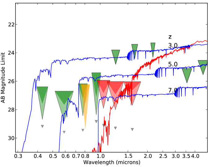
Figure 2.— Limiting magnitudes of CANDELS photometry compared to existing photometry and to the SEDs of model blue and red galaxies. HST observations are shown in two-toned triangles. Each triangle encodes three brightness limits. The bottoms of the light-colored inverted triangles are $5\sigma$ point-source limits for Deep data. The bottoms of the darker triangles show the approximate $5\sigma$ limits for aperture photometry of a fiducial Lyman-break galaxy with a half-light radius of $0.25^{\prime\prime}$, also in Deep data. The tops of the triangles show the approximate $5\sigma$ limits for LBGs in the CANDELS/Wide survey using the exposure times from Table 6 (except for F814W, see below). The green triangles at left show the GOODS/ACS data ($BViz$), the red triangles are for WFC3/IR ($YJH$). The yellow triangles denote CANDELS F814W, with the triangle bottoms corresponding to the fiducial 28 ks exposure in CANDELS/Deep and the top corresponding to a 1-orbit exposure. The points of the solid green triangles in the IR show point-source depths (valid for distant galaxies) for the GOODS VLT ISAAC $JHK$ observations (Retzlaff et al. 2010) and the GOODS Spitzer IRAC data at 3.6$\micron$ and 4.5$\micron$ (Dickinson et al. 2003). The blue SEDs are for $L^{*}$ Lyman-break galaxies at redshifts $z=3,5,$ and 7; the red SED shows a maximally old galaxy at $z=3$ with rest-frame $M_{V}=-21$ mag. For comparison, we also plot the $5\sigma$ sensitivities of the deepest existing HST images (gray triangles), covering the much smaller areas of the HUDF ($BViz$) and the HUDF09 ($YJH$) as reported by Oesch et al. (2011).

Figure 3.2 illustrates the three-tiered observing strategy for distant objects, and Table 3 sets forth estimated numbers of sources in various redshift and magnitude ranges. Based on the LFs of Bouwens et al. (2011b) and McLure et al. (2011), we anticipate finding hundreds of galaxies at $z\approx 7$ and $z\approx 8$ down to $H=27.9$ mag in CANDELS/Deep (green areas in Fig. 3.2). These objects also have the deepest available observations from Spitzer, Chandra, Herschel, the VLA, and other major facilities, which is important if we are to have any near-term hope of constraining their stellar populations, dust content, and AGN contribution.

CANDELS/Wide is designed to firm up measurements of brighter high-$z$ galaxies over a larger area. The Wide survey consists of two orbits of $J$+$H$, accompanied by four effective parallel orbits in $V$+$I$ over nearly three-quarters of the area (see a sample Wide layout in Fig. 7). The Wide filter depths are well matched to each other and to Spitzer/SEDS for detecting LBG galaxies in the range $z\approx 6.5$–8.5 down to $M_{\rm UV}\approx-20.0$ mag ($H\approx 27.0$ mag; yellow regions in Fig. 3.2). Several hundred such objects are expected. More precise redshifts will eventually require either spectra or adding $z$+$Y$ photometry, but the number density is well matched to current multi-object spectrographs. The Wide portions within GOODS, including ERS in GOODS-S, already have $z$-band imaging and already or soon will have $Y$-band imaging.

Eventual spectroscopic confirmation of galaxy redshifts at $z\gtrsim 7$ will be challenging but not impossible. For $J=27$ mag at $z=8$, a Ly$\alpha$ line with rest-frame equivalent width 30 Å yields a line flux of $4\times 10^{-18}$ erg s^-1 cm^-2, which approaches the present capabilities of near-IR spectroscopy. Current attempts have already yielded plausible single-line detections (Lehnert et al. 2010; Vanzella et al. 2011) and useful upper limits (Fontana et al. 2010). As part of CANDELS itself, there are opportunities for spectroscopic confirmation of high-$z$ candidates with grism observations that will be taken as part of the SN follow-up observations (see §3.6). Ultimately, objects at the Spitzer/SEDS sensitivity limit of $\sim 26$ mag should be spectroscopically accessible with JWST.

Observational requirements: The prime goal for Deep data is to reach 1 mag below $L^{\ast}$ at $z=8$ with $5\sigma$ accuracy, corresponding to $M_{\rm UV}\approx-19.0$ mag and hence $H=27.9$ mag (see green regions in Fig. 3.2). All three $YJH$ filters are required in the Deep program for secure detection and redshifts of the faintest galaxies. This strategy complements the HUDF09 (GO-11563; P.I. Illingworth), which used the same three filters, going $\sim 1.1$ mag deeper, but over $1/10$ the area. Our SED-fitting simulations suggest that achieving secure redshifts further requires $I_{814}$ data to be 1.5 mag deeper than $YJH$, and thus a minimum total exposure time in F814W of 28 ks in the Deep regions. Placing that much $I$-band exposure time in ACS parallels uniformly across both Deep regions is a major driver for the CANDELS observing strategy (§6.2).

The required area of the Deep fields is set by various counting statistics. First, the horizontal lines in Figure 3.2 correspond to counting 10 objects per mag, which is roughly the number needed to reduce Poisson noise below cosmic variance (§5.3). Increasing the area of any one tier of the survey extends its “sweet spot” downward and to the left. A basic requirement is that all three tiers — HUDF, Deep, and Wide — need to be large enough to make their sweet spots overlap. Figure 3.2 shows that this has been achieved with the adopted survey sizes. Second, observing only half of each GOODS field in the Deep program yields cosmic-variance uncertainties that are only 20% worse than two whole GOODS fields, at a savings of half the observing time. As shown in §5.3, the resulting cosmic variance for $6.5<z<7.5$ galaxies in the Deep survey is $\sim 20$%, sufficient to detect number density changes from bin to bin of a factor of two at $3\sigma$.

In the Wide program (yellow regions in Fig. 3.2), two orbits total in $J$+$H$ reach to 27.0–27.1 mag in each filter individually, which corresponds to $L^{\ast}$ for galaxies at $z\gtrsim 7$ . The prime goal of Wide is to return a rich sample of luminous high-$z$ candidate galaxies for future follow-up observations. A total field size in Deep+Wide of 0.22 deg² is required to obtain a total of $\sim 30$ bona fide $z=6.5$–8.5 galaxies to $H=26$ mag and 200–400 galaxies to $H=27$ mag. If divided into several separate fields, the resulting cosmic variance is again $\sim 20$% per $\delta z=1$.

(CD2) Constrain star-formation rates, ages, metallicities, stellar masses, and dust contents of galaxies at the end of the reionization era, $z\approx 6$–10. Tighten estimates of the evolution of stellar mass, dust, and metallicity at $z=4$–8 by combining WFC3/IR data with very deep Spitzer/IRAC photometry.

Existing data have revealed tantalizing trends in the stellar populations of high-redshift galaxies, which are providing important clues to the progress of star formation and its dependence on galaxy properties. Bouwens et al. (2010b) claim that the UV continuum slopes of galaxies at $z\approx 7$ are very steep, implying that these galaxies are younger, less dusty, and/or much lower in metallicity ($<10^{-3}\,Z_{\odot}$) than LBGs at lower redshift. Furthermore, the data, though noisy, show a constant ratio of SFR to stellar mass at all redshifts $z>3$ (González et al. 2010). This constant specific SFR conflicts strongly with the traditional assumption that SFRs of galaxies are either constant or exponentially declining and indeed implies that SFR and stellar mass are both exponentially increasing (Papovich et al. 2011). This implies that the long-sought era of galaxy turn-on has finally been detected, at redshifts that are accessible to Hubble.

CANDELS data are crucial for following up these results. At $z>6$, current trends are based on fewer than 100 galaxies spanning a small dynamic range in luminosity. CANDELS observations will increase both the number of available galaxies and the dynamic range. Estimates of stellar masses at $z\approx 6$–8 connect these galaxies to reionization by constraining the total number of ionizing photons emitted by previous stellar generations and to their progenitors and descendants at other redshifts. At $z<6$, the combination of WFC3/IR and SEDS/IRAC bridges the Balmer break and removes much of the degeneracy between dust and age. Color criteria also reveal whether there are non-star-forming galaxy candidates lurking at these redshifts. Such searches have been severely hampered by the lack of adequate NIR data, and the few reports of massive aging galaxies at high $z$ are highly controversial (Mobasher et al. 2005; Wiklind et al. 2008; Chary et al. 2007; Dunlop et al. 2007). Finally, better photometric redshifts from more accurate SEDs will inform all of this work.

Observational requirements: Most of the requirements for modeling high-$z$ stellar populations are already met by goal CD1. The main new requirement is that fields have both deep optical images and deep Spitzer/IRAC. The latter reaches rest-frame $B$ to $V$ and is crucial for measuring stellar masses (see Fig. 2). Choosing fields within the Spitzer/SEDS survey satisfies this need, increasing the total sample of galaxies at $z>6$ with suitably deep IRAC+WFC3/IR data by tenfold. Other high-$z$ WFC3/IR surveys (e.g., those with WFC3/IR in parallel) lack Spitzer imaging as well as all the other multi-wavelength data needed for excellent photometric redshifts and SED modeling. A few dozen bright LBGs at $z>6$ will be visible individually in the Spitzer/SEDS Deep regions, and stacking can extend IRAC constraints to fainter samples (Labbé et al. 2010; Finkelstein et al. 2011).

(CD3) Measure fluctuations in the near-IR background light, at sensitivities sufficiently faint and angular scales sufficiently large to constrain reionization models.

Most galaxies prior to reionization — including those dominated by Population III stars — are too faint to be detected individually even with WFC3, but they contribute to the spatial fluctuations of the extragalactic background light (EBL). First-light galaxies should be highly biased and trace the linear regime of clustering at scales of tens of arcminutes when projected on the sky (Cooray et al. 2004; Fernandez et al. 2010). Recent attempts to detect the EBL have been controversial. Kashlinsky et al. (2005) detected fluctuations in deep Spitzer/IRAC observations and interpreted these as evidence for a large surface density of reionization sources. Subsequent work, which stacked NICMOS data (Thompson et al. 2007a, b) at at the positions of $z_{850}\approx 27$ sources (Chary et al. 2008), suggested that about half the power in the Spitzer fluctuations can be attributed to $z\approx 1.5$ galaxies.

The deepest current observations appear to show a declining SFR density at $z>6$ among bright LBGs. This could imply that galaxies below the WFC3/IR detection limit are producing the bulk of the ionizing photons. Alternately, the very small volume surveys that probe these redshifts (such as the HUDF) could be probing unusually low-density parts of the Universe due to bad luck with cosmic variance. Observations of lensing cluster fields trace too small a volume and suffer from uncertainties in magnification that vitiate robust galaxy LFs at the faint end. Prior to JWST, EBL fluctuations in WFC3/IR data are arguably the most powerful probe of very faint sources responsible for reionization.

Observational requirements: EBL measurements are essentially impossible from the ground because of high and variable sky background. EBL measurements are best done in fields with deep ACS observations, where simultaneous optical and near-IR fluctuation measurements can be used to constrain the redshift distribution of the faint sources. Relative to existing Hubble near-IR deep fields, CANDELS observations will increase the angular scales over which the fluctuations can be measured by a factor of 2–3, which will enable the contribution of the first-light sources to be measured at $\sim 0.8$ nW m^-2 sr^-1, at wavelengths where the contribution of these sources to the EBL is thought to peak. This is illustrated in Figure 3.2, which shows the power spectrum of fluctuations on arcminute scales expected if the reionization sources trace linear clustering on large scales at $z\approx 10$ (green curve), along with the predicted uncertainties from CANDELS and the measured values from deep NICMOS observations (Thompson et al. 2007a). The observing strategy and data reduction will require careful attention to flatfielding, scattered light, bad pixels, and latent images from previous observations.

Fast-reionization scenarios, involving rapid ($\Delta z\approx 2$–4) transition from a neutral to an ionized universe ending at $z\approx 6$–7, are consistent with the WMAP measured optical depth and the Sloan observations of the Gunn-Peterson trough in $z\approx 6$ QSOs (Chary & Cooray, in prep.). Because the redshift range is narrow and the sources are brighter than in scenarios extending to higher redshift, the EBL fluctuations are expected to be stronger in such fast scenarios. A nondetection of the fluctuations in the proposed data would point toward a more extended epoch of reionization with significant contributions from fainter sources.

(CD4) Use clustering statistics to estimate the dark-halo masses of high-redshift galaxies with double the area of previous Hubble surveys.

The biggest challenge in galaxy formation studies is relating the visible parts of galaxies to the properties of their invisible dark matter halos. Galaxy clustering statistics such as two-point correlation functions can provide strong constraints on the masses of the dark matter halos that harbor a given observed population (Conroy et al. 2006; Lee et al. 2006, 2009). This is done by taking advantage of our excellent understanding of the clustering properties of dark matter halos, and adopting a prescription to populate halos with galaxies (often called “Halo Occupation Distribution” or “Conditional Luminosity Function” formalism (e.g., van den Bosch et al. 2007). The CANDELS fields will likely be too small for clustering to yield strong constraints at the highest redshifts, but it should be possible to apply these kinds of techniques at the lower range of the “cosmic dawn” redshift window ($z\approx 6$–7), which is still very interesting.

Observational requirements: Cosmic variance is a dominant source of error in clustering measurements for small-area surveys, and it can be mitigated in two ways. The most effective is to break up the imaging area into several separate regions that are widely distributed on the sky. Secondly, elongated field geometries sample larger scales that are more weakly correlated, and thus suffer less cosmic variance than compact geometries. However, the narrowest field dimension should not drop too close to the correlation length $r_{0}$, which at moderate redshifts is a few Mpc. The adopted sizes and layouts of the CANDELS fields are well optimized in these respects.

Extragalactic background fluctuations. The green curve is a model (Cooray et al. 2004; Trac & Cen 2007) that provides the star formation necessary to reionize the universe by $z\approx 7$–8. The purple points are the Thompson et al. (2007a) measurement of fluctuations in the NICMOS HUDF. The red points with error bars illustrate the proposed CANDELS measurements, which are set to match the NICMOS measurements on small scales and the predicted linear fluctuations due to reionization sources on scales of $10^{\prime}$. Under these assumptions, the measurements would yield a $7\sigma$ detection of the expected spatial clustering at scales larger than $1^{\prime}$. The dashed line shows the “shot noise” Poisson fluctuations due to the finite number of faint galaxies. The solid curve shows the linear clustering of halos at $z\approx 10$ projected on the sky.

(CD5) Search the deep WFC3/IR images for AGN drop-out candidates at $z>6$–7 and constrain the AGN luminosity function.

In the very early universe, AGNs are expected to play a significant role both in the evolution of the first galaxies and the reionization of the universe. Wide-area optical/NIR surveys have found QSOs out to $z\approx 6$ (e.g., Fan et al. 2003) but are limited to the most luminous and massive objects; the populations of both more typical ($L^{*}$) and obscured AGNs are almost completely unknown. Deep X-ray surveys can readily detect $L^{*}$ (and fainter) AGNs at $z>6$, but extremely deep near-IR data are required to verify them. Candidate high-redshift AGNs have already been postulated among the “EXOs”: X-ray sources without optical counterparts even in deep HST/ACS images (Koekemoer et al. 2004). Drop-out techniques should be effective for identifying high-$z$ AGNs, just as for galaxies; ultra-deep near-IR data are critical for distinguishing true high-$z$ candidates from interlopers via SED fitting.

Semi-analytic models make significantly varying predictions of the low-luminosity AGN population at high $z$, differing by over an order of magnitude (e.g., Rhook & Haehnelt 2008; Marulli et al. 2008). CANDELS will distinguish decisively between these models: we estimate $\sim 10$ AGNs at $z>6$ in the Wide survey accounting for the X-ray detection limits in all fields, but with a factor $\sim 2$–3 uncertainty in each direction depending on which evolutionary model is employed (Aird et al. 2008; Brusa et al. 2009; Ebrero et al. 2009). Once appropriate candidates have been found, it will be possible to probe the physical processes associated with the formation of the first AGNs. For example, if early black hole growth is mainly merger-driven (Li et al. 2007), one would expect both coeval star formation and a substantial stellar population associated with the AGN. CANDELS multi-wavelength data will provide the first clues to this.

Observational requirements: Many of the requirements for detecting the host galaxies of these high-$z$ AGNs are already met by the requirements for goal CD1, namely the combination of area and depth in $J$+$H$ as well as the bluer bands, to enable robust selection of a sufficient number of drop-out sources. Additional requirements specifically related to high-$z$ AGNs are the existence of sufficiently deep X-ray imaging, to enable selection of $L^{*}$ AGNs up to at least $z\approx 6$–7, as well as deep Spitzer mid-IR imaging for detection of warm dust emission from the AGN torus the can expand the sample to obscured/Compton-thick sources. These datasets exist to varying depths across all 5 CANDELS fields, thereby enabling a sufficient number of high-$z$ AGNs to be identified in conjunction with the deep HST imaging.

3.3. Galaxies and AGNs: Cosmic High Noon

Our use of the term “cosmic high noon” covers roughly $z=1.5$ to 3. This epoch features several critical transformations in galaxy evolution, as follows. (1) The cosmic SFR and number density of luminous QSOs peaked. (2) Nearly half of all stellar mass formed in this interval. (3) Galaxies had much higher surface densities and gas fractions than now, and the nature of gravitational instabilities and the physics of star formation may have been different or more extreme. (4) Despite the overall high SFR, SFRs in the most massive galaxies had begun to decline, and red central bulges had appeared in some star-forming galaxies. Mature, settled disks were starting to form in some objects.

Theoretical models of galaxy assembly suggest that the $z\approx 2$ era was particularly important. The cosmic-integrated accretion rate of fresh gas likely peaked at $z\approx 2$, and stellar and AGN-powered outflows were probably also at maximum strength. Certain massive galaxies may have been transitioning from accreting gas via dense, filamentary “cold flows” to forming a lower density halo of hot gas (Kereš et al. 2005; Dekel & Birnboim 2006), susceptible to heating by radio jets powered by the recently formed population of massive black holes, and this transition may be a factor in the onset of “senescence” among massive galaxies. Galaxy mergers may also be a driving force in the assembly, star-formation, and black-hole accretion of massive galaxies at this epoch, turning star-forming disks into quenched spheroidal systems hosting massive black holes (Hopkins et al. 2006).

The above complex of phenomena make cosmic high noon a unique era for studying processes that transformed the rapidly star-forming galaxies of cosmic dawn into the mature Hubble types of today. We outline below four science goals to be addressed at this redshift.

(CN1) Conduct a mass-limited census of galaxies down to $M_{*}=2\times 10^{9}{\rm M}_{\odot}$ at $z\approx 2$ and determine redshifts, SFRs, and stellar masses from broadband spectral-energy distributions. Quantify patterns of star formation versus stellar mass and other variables and measure the cosmic-integrated stellar mass and star formation rates to high accuracy.

CANDELS measurements will be used to compare the universally averaged SFR and the stellar mass density over cosmic time. Current estimates of integrated cosmic SFR disagree with the observed stellar mass density by roughly a factor of two at redshifts $z<3$ (Hopkins & Beacom 2006; Wilkins et al. 2008), leading to suggestions that the stellar initial mass function may be non-universal. However, better constraints on the properties of low-mass galaxies could also resolve this discrepancy (Reddy et al. 2008). Therefore it is critical to push measurements of the stellar mass function well below current ground-based data stellar-mass limits of $10^{10}$ M_⊙ at $z\approx 2$ (e.g., Marchesini et al. 2009).

CANDELS will also be used to study how star formation proceeds and is shut down in individual galaxies during this epoch of rapid galaxy assembly. The individual SFRs in star-forming galaxies correlate closely with their stellar masses in a narrow “star-forming main sequence” seen at $z<3$ (Brinchmann et al. 2004; Noeske et al. 2007; Daddi et al. 2007b; Pérez-González et al. 2008). The zero-point of this sequence declines steadly from $z\approx 2.5$ to $z\approx 0$ (Noeske et al. 2007; Daddi et al. 2007b), resulting in the rapid decline of the cosmic SFR over this epoch (Madau et al. 1996; Lilly et al. 1996). As early as $z\approx 3$, star formation begins to shut down rapidly in massive galaxies (e.g., Juneau et al. 2005; Papovich et al. 2006), leading to the formation of a quenched “red sequence” that grows with time (Bell et al. 2004; Faber et al. 2007; Brown et al. 2007). Improved photometric redshifts, stellar masses, and SFRs at cosmic high noon will place tighter constraints on the origin and evolution of the SFR-stellar mass correlation and galaxy quenching.

Plotted is the difference between two sets of photometric redshifts for galaxies in the ERS region. One set uses the best available space-based and ground-based photometry at optical and near-IR wavelengths. The second set substitutes new $YJH$ data from WFC3/IR. For brighter galaxies ($H<25$ṁag), the substitution makes little difference, but for fainter galaxies ($H>25$ mag), photometric redshifts change significantly with the newer (and presumably more accurate) WFC3/IR values.

Observational requirements: The above science goals require a mass-limited census of galaxies down to $2\times 10^{9}$ M_⊙ out to $z\approx 2.5$. The reddest galaxies at this mass will have $H\approx 27.3$ mag and will be detected in the Deep regions only. We estimate finding $\sim 500$ objects in total above $2\times 10^{9}$ M_⊙ in the redshift range $z=1.5$–2.5 (Table 3). The Wide survey limit is roughly 1 mag brighter and will sample $\sim 5000$ objects above $5\times 10^{9}$ M_⊙. Mass limits for blue galaxies are nearly ten times smaller. Both Deep and Wide survey limits improve several-fold over current limits. As shown in §5.3, we expect that CV errors with the current survey design will be $<$20% for both massive galaxies ($m_{\rm star}\approx 10^{11}$ M_⊙) in the Wide survey and also for low-mass galaxies ($m_{\rm star}\approx 2\times 10^{9}$ M_⊙) in the Deep regions, each for redshifts $z=1.5$–2.5.

High quality photometric redshifts and SEDs are needed for all galaxies, requiring multi-band WFC3/IR data, ACS parallel imaging and other ancillary data deep enough to match WFC3/IR for all galaxy colors. At CANDELS faintest levels, photometric redshifts will be the main source of redshifts for the foreseeable future; $YJH$ filters span the Balmer/4000 Å break at $z\approx 2$, which makes them crucial for photometric redshifts (Figure 2). Figure 3.3 compares photometric redshifts with and without recent high-quality Hubble ERS $YJH$ photometry. Brighter than $K=24.3$ mag, there is little difference, but below $K=24.3$  mag, the differences can be huge, particularly at cosmic high noon. Better $YJH$ data will also tighten SEDs across the Balmer break, helping to disentangle the age-dust degeneracy and improving stellar population estimates from SED fitting. Existing GOODS ACS images do not reach faint red galaxies at $z\approx 2$, and thus the $\gtrsim 28$ ks F814W parallels in the Deep fields, designed for high-$z$ galaxy detection (see goal CD1, §3.2), are essential.

Combined with SEDS/IRAC photometry from Spitzer, CANDELS will obtain good stellar masses for all $z\approx 2$ galaxies regardless of color down to the $H$-band magnitude limit (Fig. 2). The resulting stellar-mass inventory should be a considerable advance over present data, especially when paired with improved SFRs from HST rest-frame UV, Spitzer, and Herschel mid/far-IR data available in all CANDELS fields (see §5).

(CN2) Obtain rest-frame optical morphologies and structural parameters of $z\approx 2$ galaxies, including morphological types, radii, stellar mass surface densities, and quantitative disk, spheroid and interaction measures. Use these to address the relationship between galactic structure, star-formation history, and mass assembly.

Previous HST studies have characterized the rest-frame UV structure of galaxies at $1.5<z<2.5$ below the Balmer break. The impression from these images is that a “galactic metamorphosis” occurred near $z\approx 1.5$: galaxies at earlier times displayed a much higher degree of irregularity than later generations (e.g., Driver et al. 1995; Abraham et al. 1996; Giavalisco et al. 1996). However, Figure 1 shows that rest-frame UV images can be biased toward young stars and may not show the true underlying structure of the galaxy, which is better seen in the older, redder stars. Recent results using WFC3 have demonstrated the importance of high-resolution NIR for characterizing morphology of the massive galaxies in this redshift range (Conselice et al. 2011b; Law et al. 2011). Covering much larger area than these early WFC3/IR studies, CANDELS will more comprehensively measure the frequency of disk, spheroidal and peculiar/irregular structures in rest-frame optical light for $1.5<z<3$ galaxies, as evidenced by visual properties and quantitative measures such as Sersic index, bulge-to-disk ratio, axial ratio distributions, and concentration/Gini-M₂₀.

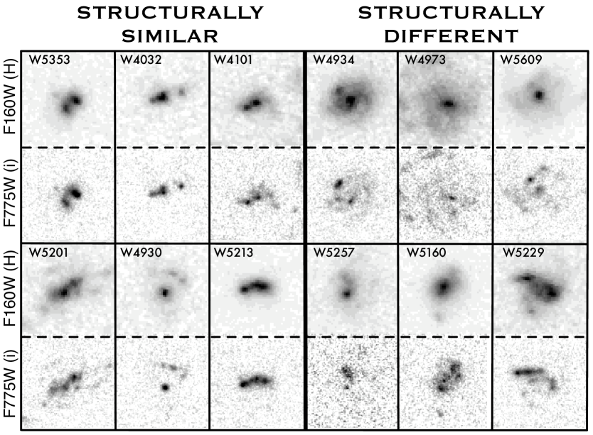
Figure 3.— Clumpy $z\approx 2$ galaxies from WFC3 Early Release Science (ERS) images taken in F160W (2-orbit depth) versus F775W (3-orbit depth). Object IDs are from the FIREWORKS (Wuyts et al. 2008) and MUSYC (Cardamone et al. 2010) catalogs. Galaxies are arranged in two groups. On the left are objects for which the two images look quite similar, while objects on the right look substantially different. Cases like W4934, W4973, and W5609 on the right appear to have underlying disks composed of older stars and may be candidates for inherently regular galaxies in which clump formation has occurred via in situ disk instabilities. Cases on the left like W4032, W5201, and W5353 lack such underlying disks and are more likely to be separate galaxies now merging. F160W also highlights the presence and location of central potential wells, as in W4934, W5160, and W5229.

Theoretical models of disk formation make quantitative predictions for disk scaling relations and their evolution with cosmic time (Somerville et al. 2008a; Dutton et al. 2011), which may be compared with the rest-frame optical sizes that will be measured by CANDELS. The distribution of disk axial ratios and the frequency of bars and spiral structures will be used to probe the degree of disk settling and the development of dynamically cold and gravitationally unstable disk structures (Förster Schreiber et al. 2009; Ravindranath et al. 2006). Radii also yield stellar mass surface densities, which have been implicated as a threshold parameter for quenching and evolution to the red sequence (Kauffmann et al. 2003; Franx et al. 2008). We will attempt to link the structural and dynamical properties of disks with their SFRs and to confront the latest theoretical ideas for the processes that regulate and stimulate star formation with these observations.

Major mergers occupy a central role in hierarchical theories of galaxy formation, and are a favorite mechanism for building spheroids, triggering BH growth and igniting starbursts (e.g., Sanders et al. 1988; Hopkins et al. 2006; Somerville et al. 2008b). Quenching by mergers and associated feedback (e.g., Hopkins et al. 2006) tends to destroy disks, whereas quenching through declining accretion (or “strangulation”) tends to preserve them. Measuring disk and spheroid fractions of red sequence galaxies versus mass and time is therefore a clue to how galaxies have transited to the red sequence at different epochs.

Passive galaxies must have evolved substantially along the red sequence as well. Galaxies with very low specific SFRs are present to at least $z=2.5$ but with sizes that are much smaller than those of nearby ellipticals of the same mass (e.g., Daddi et al. 2005; Trujillo et al. 2007; Cimatti et al. 2008; van Dokkum et al. 2008). If these sizes are correct, the implication is that massive spheroids must have accreted considerable stellar mass after $z\approx 2$ and that their extended stellar envelopes grew by dry minor mergers (Naab et al. 2009; van Dokkum et al. 2010). These outer envelopes may be quite red and can be observed using stacked images from WFC3/IR, from which evolution in both radii and concentration indices can be measured.

Direct measurements of major and minor merger rates are also needed to inform theory, especially at $z\approx 2$, where QSOs peak. Galaxy interactions, disturbances, and mergers will be identified directly in the CANDELS images using both visual and quantitative methods such as CAS (Conselice et al. 2003) and Gini/M₂₀ (Lotz et al. 2004). Detailed numerical simulations of merging galaxies are able to predict the visibility of mergers using different methods (e.g., Lotz et al. 2008; Conselice 2006). Thus observed galaxy merger fractions may be converted into major and minor merger rates and compared to theoretical predictions.

Comparison of galaxy structural parameters derived from Wide-quality 4/3-orbit images (synthesized from HUDF F160W) vs. values obtained from the full 28-orbit data. In order, the quantities plotted are effective radius, Sersic index, axial ratio, Gini, and M₂₀. The adopted useful limit for Wide data is the vertical dotted line at $H=24.0$ mag; Deep data will go 0.7 mag fainter, which is $M_{*}\approx 2\times 10^{10}$ M_⊙ at $z\approx 2.5$ (see Table 3).

Observational requirements: Answering these questions requires measuring accurate radii and axial ratios, tracking spheroids and disks, searching for substructure in the form of bars and spiral arms, and identifying merger-induced distortions. Given the small angular sizes of most $z\approx 2$ galaxies, detailed structural parameters depend on extracting the highest possible spatial resolution from WFC3/IR images, which requires multiple exposures and fine dithering. The WFC3 Y, J, and H bandpasses will be used to track evolution of galaxy structure at a uniform rest-frame optical ($\sim B$-band) wavelength from $z\approx 1.5$ to $z\approx 3$.

The quality of structural data to be expected in the Wide program is illustrated in Figure 3.3, which shows several quantitative morphological statistics (effective radius, Sersic index, axial ratio, Gini, and M₂₀) computed on 4/3-orbit F160W data compared with the same quantities computed with 28-orbit data from the HUDF. The vertical line is the adopted “acceptable” limit, which is at $H=24.0$ for Wide, and $H=24.7$ mag for Deep. These correspond to stellar masses of $4\times 10^{10}$ M_⊙ and $2\times 10^{10}$ M_⊙ respectively at $z=2.5$ (Table 3), which is deep enough to capture most galaxies transiting to the red sequence if they do so at a similar mass as the observed transition mass in the local Universe ($\sim 3\times 10^{10}$ M_⊙, Kauffmann et al. (2003)).

Interpolating in Table 3 predicts $\sim 225$ galaxies in the Deep regions above this level in the range $z=1.5$–2.5. The Wide program will mainly sample rarer objects such as massive galaxies and mergers. The expected limit in Wide is two times brighter ($H=24.0$), and $\sim 1200$ objects are expected above this level in the same redshift range. If major mergers involve roughly $\geq$ 10% of galaxies at $z\approx 2$ (Lotz et al. 2008), $\geq$75 bright mergers will be available for detailed morphological modeling in Wide+Deep.

(CN3) Detect galaxy sub-structures and measure their stellar masses. Use these data to assess disk instabilities, quantify internal patterns of star formation, and test bulge formation by clump migration to the centers of galaxies.

Many star-forming galaxies at $z\approx 2$ have compact sizes, high surface densities and high gas fractions (Tacconi et al. 2010), and exhibit star-forming clumps more massive than local star clusters (Elmegreen et al. 2009). This is qualitatively consistent with state-of-the-art cosmological simulations, which indicate that massive galaxies can acquire a large fraction of their baryonic mass via quasi-steady cold gas streams that penetrate effectively through the shock-heated hot gas within massive dark matter halos (e.g., Kereš et al. 2005; Dekel & Birnboim 2006; Dekel et al. 2009). Angular momentum is largely preserved as matter is accreted, early disks survive and are replenished, and instabilities in fragmenting disks create massive self-gravitating clumps that rapidly migrate towards the center and coalesce to form a young bulge (Dekel et al. 2009; see also Noguchi 1999; Immeli et al. 2004; Bournaud et al. 2007; Elmegreen et al. 2008).

Testing this picture requires distinguishing between clumps generated from internal disk instabilities and substructure accreted by external interactions and mergers. As shown in Figure 3, high-spatial resolution multi-band HST images may be able to do this, permitting us to classify disturbed galaxies into the two camps (though this needs to be checked with simulations). Rest-frame UV images from ACS provide a map of where unobscured stars are forming, while rest-frame optical images from WFC3/IR give improved dust maps and clump stellar masses. The numbers, spatial distribution, stellar masses and SFRs of the clumps can then be compared to cosmological simulations of forming galaxies to test the new paradigm of cold streams and their impact on disk star formation.

Observational requirements: Deep and high-spatial resolution imaging is needed to extract reliable clump information, and may require deconvolved high signal-to-noise ratio ($S/N$) Deep WFC3/IR images for resolved stellar population studies. A full inventory of star-formation properties for clumpy star-forming galaxies will require both WFC3/IR and ACS/optical imaging as well as extensive ancillary data on integrated SEDs, SFRs, emission line strengths, and dust temperatures from a wide range of ground and space telescopes.

(CN4) Conduct the deepest and most unbiased census yet of active galaxies at $z\gtrsim 2$ selected by X-ray, IR, optical spectra, and optical/NIR variability. Test models for the co-evolution of black holes and galaxies and triggering mechanisms using demographic data on host properties, including morphology and interaction fraction.

The discovery of the remarkably tight relation between black hole masses and host spheroid properties (Magorrian et al. 1998; Gebhardt et al. 2000; Ferrarese & Merritt 2000; Häring & Rix 2004) has given birth to a new paradigm: the co-evolution of galaxies and their central supermassive black holes (BHs). However, since only a small fraction of galaxies appear to be building BHs at any instant, it is unclear how the galaxy-black hole connection was either first established or subsequently maintained. One suggested mechanism is major mergers, which scramble disks into spheroids, feed BHs, and quench star formation via AGN or starburst driven winds (e.g., Sanders et al. 1988; Hopkins et al. 2006). A testable feature of this model is the strong merging and disturbance signatures predicted for AGN host galaxies, as shown in Figure 4. The total Wide volume in the 1.6 Gyr period $1.5<z<2.5$ contains roughly 3000 galaxies with stellar mass $>10^{10}$ M_⊙ (Table 3). Models predict that a typical galaxy suffered one major merger during this period. If this picture is correct, we would therefore expect $\gtrsim$300 galaxies in the highly disturbed phase and 300 in the visible QSO phase. Hubble imaging has not thus far shown much evidence for excess merger signatures in X-ray sources at $z\approx 1$ (Grogin et al. 2005; Pierce et al. 2007), but triggering processes in brighter QSOs, which are more common at $z\approx 2$, may differ. A second prediction, though not unique to this model, is that massive black holes should be found only in galaxies possessing major spheroids. Suggestion of this from the GOODS AGN hosts at $z<1.3$ (Grogin et al. 2005) may now be scrutinized over a much broader redshift range, $z\lesssim 3$, with CANDELS.

Figure 4.— Top panels show simulated rest-frame $urz$ images of a gas-rich major merger. The image was created using a hydrodynamic simulation of a binary galaxy merger including star formation, black hole accretion, and AGN feedback (Di Matteo et al. 2005). The simulation results were post-processed through the dust and radiative transfer code Sunrise (Jonsson et al. 2010). Successive merger stages are labeled (1–6). The middle and bottom panels show the predicted IR luminosity and rest-frame optical asymmetry vs. merger stage for the same simulation. This picture predicts that the maximal asymmetry should be measured during the relatively early stages of the merger, while the object would be identified as an obscured or optical QSO in the late stages, when the two nuclei may have largely coalesced and faint tidal features may be the only remaining signs of morphological disturbance (see also Hopkins et al. 2008).

The CANDELS fields, with their superior X-ray imaging area and depth (now extended to an unprecedented 4 Ms in GOODS-S), plus multi-epoch ACS imaging, ultra-deep Spitzer, Herschel, and radio coverage (see §5), provide by far the best data with which to identify and study distant AGNs — not only X-ray AGNs but also their heavily obscured counterparts. Between 20 and 50% of $z\approx 2$ galaxies may host a Compton-thick AGNs undetected in X-rays (Daddi et al. 2007a) but appearing as luminous IR power-law SEDs in Spitzer and Herschel data (Alonso-Herrero et al. 2006; Donley et al. 2008, Juneau & Dickinson, in prep.). These highly obscured sources might hide key phases of BH growth. They might also be the very ones most likely to show mergers and asymmetries (Figure 4; see also Hopkins et al. 2008). The multi-wavelength ancillary data combined with CANDELS HST imaging will also allow us to connect and compare this active BH accretion phase of galaxy formation to active star-formation phases that produce ultra-luminous IR and sub-mm galaxies (e.g., Donley et al. 2010; Pope et al. 2008; Alexander et al. 2008; Coppin et al. 2008).

Table 4Number of X-ray Sources

Field	Area	Telescope	Exposure	Total number	Number in	$F_{lim}$
	arcmin2			in field	$z=1.5$–2.5	erg s-1 cm-2
COSMOS	176	Chandra	200 ks	106	10	$2\times 10^{-16}$
EGS	180	Chandra	800 ks	240	40	$3\times 10^{-17}$
GOODS-N	132	Chandra	2 Ms	175	32	$2\times 10^{-17}$
GOODS-S	124	Chandra	4 Ms	317	90	$1\times 10^{-17}$
UDS	176	XMM	100 ks	70	5	$6\times 10^{-16}$

Note. — Table shows numbers of X-ray sources, in total over each CANDELS field and in the $z=1.5$–2.5 redshift bin. The former is based on actual counts, while the latter is based on extrapolations from sources with measured redshifts and is quite uncertain.

Observational requirements: In addition to multi-wavelength data for AGN identification, co-evolution studies need the redshifts, stellar masses, stellar population and dust data, bulge and disk fractions, and disturbance indicators to be obtained with the CANDELS HST data. X-ray AGNs at $z\approx 2$ are found mainly above $\sim 2\times 10^{10}$ M_⊙ (Kocevski et al., in prep.), which is fortuitously equal to the limit for detailed morphologies in Deep data (goal CN2 above). However, AGNs are rare, and the larger area of the Wide survey, even though it does not go quite as deep, is clearly crucial for obtaining a valid sample of these objects.

Predicted numbers of X-ray objects in CANDELS fields are given in Table 4 based on current observed X-ray counts. If all CANDELS fields were surveyed to a depth of 800 ks (as in EGS), roughly 200 X-ray AGNs would be found within the CANDELS area in the range $z=1.5$–2.5 (Table 3). Figure 4 predicts that the number of obscured AGNs should be similar. Due to their extremely red colors, some 25% of obscured AGNs lack ACS counterparts, and 60% lack ground-based NIR counterparts. WFC3/IR is the only hope for imaging such objects in the near future. Finally, multi-epoch ACS data in all fields, especially GOODS, will be unparalleled for AGN variability studies.

3.4. Ultraviolet Observations

GOODS-N is in the HST continuous viewing zone (by design). Thus we can boost HST efficiency by using the bright day-side of the orbit to observe in the UV with WFC3/UVIS (specifically the F275W and F336W filters). We conservatively plan on 100 orbits with UV observations, but this could be as high as $\sim 160$ orbits if we are able to make use of all the available opportunities.

Because these observations are read-noise limited, we have chosen to bin the UVIS data to reduce read noise and gain $\sim 0.5$ mag of sensitivity in each filter. To facilitate the selection of Lyman-break drop-outs at $z\approx 2$ and to increase the sensitivity to LyC radiation at $z\approx 2.5$, we expose twice as long in F275W as in F336W. Due to scheduling constraints, we anticipate that many of the orbits may not have full CVZ duration, and the UVIS exposure times on the day side of the orbit may be scaled back. Nonetheless, we expect to get the equivalent of $\sim 100$ orbits of UVIS imaging in the field. Depending upon final exposure times and the degradation of the UVIS detectors’ charge-transfer efficiency, we expect depths of $\sim 27.9$ and $\sim 27.7$ mag in F275W and F336W, respectively ($5\sigma$ in a 0.2 arcsec² aperture).

These data enable three important scientific investigations.

(UV1) Constrain the Lyman-continuum (LyC) escape fraction for galaxies at $z\approx 2.5$.

A composite spectrum of distant LBGs is shown in Figure 3.4 as it would appear redshifted to $z=2.4$. Overplotted are the transmission curves of the WFC3/UVIS filters being used in the GOODS-N CVZ day-side observations. At $z>2.38$, the Lyman limit shifts redward of any significant transmission in the F275W filter, and this filter therefore probes the escaping Lyman continuum radiation for galaxies in the range $2.38<z<2.55$ (where the upper limit is dictated by IGM opacity).

The composite LBG spectrum of Shapley et al. (2003) is shifted to $z=2.4$ (the spectrum at $\lambda_{\rm rest}<912$ Å is an estimate). Overplotted (with arbitrary scaling) are the transmission curves of the UVIS filters being used in the GOODS-N CVZ day-side observations. At $z>2.38$, the Lyman limit shifts redward of any significant transmission in the F275W filter. Therefore, this filter will probe the escaping Lyman continuum radiation for galaxies at $2.38<z<2.55$ (where the upper limit is dictated by IGM opacity). Also demonstrated is the ability to efficiently select star-forming galaxies via a decrement in the F275W flux due to Lyman continuum opacity from Hi in both the IGM and the interstellar medium of the galaxy (see text for details).

Within the CANDELS/Deep portion of GOODS-N, there are about 20 LBGs (depending upon final pointings and orientations) with spectroscopic redshifts at the optimal redshift ($2.38<z<2.55$) that are luminous enough ($R>24.7$, $L_{\rm UV}>0.6L^{*}$) so that the Lyman continuum escape fraction can be significantly constrained ($f_{esc,rel}<0.5$ to $3\sigma$). Because the spectroscopy is only $\sim 40$% complete, we expect to double this sample with additional spectroscopy and get strong constraints on the LyC escape fraction in a large, unbiased sample of more than 40 LBGs. (cf. Shapley et al. 2006; Iwata et al. 2009; Siana et al. 2010). Importantly, these galaxies are at redshifts that allow H$\alpha$ measurements from the ground for an independent measure of the ionizing continuum. The resolved LyC distributions will test different mechanisms for high $f_{esc}$ including SN winds (Clarke & Oey 2002; Fujita et al. 2002), and galaxy interactions (Gnedin et al. 2008).

(UV2) Identify Lyman-break galaxies at $z\approx 2$ and compare their properties to higher-$z$ Lyman-break galaxy samples.

Star-forming galaxies at $z\approx 2$ will be selected via identification of the Lyman break in the F275W passband, analogous to HST Lyman break studies at $4<z<8$ (Bouwens et al. 2007, 2010a). These data will help identify the large population of faint galaxies that are suggested by initial findings of a steep LF (Oesch et al. 2010) and provide a more accurate census of the SFR density at this epoch. Furthermore, the existing ACS GOODS data will allow an investigation of the dependence on the UV attenuation by dust as a function of UV luminosity, to compare to existing studies at higher redshift (Reddy et al. 2008; Bouwens et al. 2010b).

(UV3) Estimate the star-formation rate in dwarf galaxies at $z>1$.

It has been hypothesized that the UV background heats the gas in low-mass halos enough to prevent cooling and star formation at $z>2$, solving the missing-satellite problem (Babul & Rees 1992; Bullock et al. 2000). An important test of this idea is to measure the SFR in dwarf galaxies as a function of lookback time to see if they are beginning to form stars toward low redshift as the ionizing background decreases. CANDELS F275W observations can detect dwarf galaxies at $1<z<1.5$ forming stars at $>0.3M_{\odot}$ yr^-1.

3.5. Supernova Cosmology

Observations of high-redshift SNe Ia provided the first and most direct evidence of the acceleration of the scale factor of the Universe (Riess et al. 1998; Perlmutter et al. 1999), indicating the presence of “dark energy”. Elucidating the nature of dark energy remains one of the most pressing priorities of observational cosmology. HST and ACS have played a unique role in the ongoing investigation of dark energy by enabling the discovery of 23 SNe Ia at $z>1$, beyond the reach of ground-based telescopes (Riess et al. 2004, 2007). From these data we have learned that (1) the cosmic expansion rate was decelerating before it recently began accelerating, a critical sanity test of the model; (2) dark energy was acting even during this prior decelerating phase; (3) SNe Ia from 10 Gyr ago, spectroscopically and photometrically, occupy the small range of diversity seen locally; (4) a rapid change is not observed in the equation-of-state parameter of dark energy, $w=P/(\rho c^{2})$, though the constraint on the time variation, ${dw\over dz}$, remains an order of magnitude worse than on the recent value of $w$; and (5) the rate of SNe Ia at $z>1$ declines, suggesting a nontrivial delay between stellar birth and SN Ia stellar death (Dahlen et al. 2008).

WFC3/IR opens an earlier window into the expansion history at $1.5<z<2.5$, beyond the reach of prior HST/ACS $z$-band SN searches including GOODS and the follow-on PANS (Program 10189; PI A. Riess). CANDELS will exploit this added reach in order to test the foundations of SNe Ia as distance indicators: the nature of their progenitor systems and their possible evolution. Simultaneously and in parallel, HST will continue to find lower-redshift SNe Ia at $z>1$, which offer additional constraints on the time variation of $w$. In Figure 3.5, we show the predicted redshift distributions of SNe Ia detectable at $5\sigma$ with one-orbit HST observations separated by 52 days (approximately optimal for high-$z$ SN Ia detection) in the filters $zYJH$. CANDELS will be searching at one-orbit depth with a combination of $J+H$ exposures. Predicted redshift distributions of detected SNe Ia assuming a 52 day separation between observational epochs and assuming that the search was done entirely in each filter shown. The magnitude limit assumed for detecting SNe corresponds to the $S/N=5$ limit reached in one orbit for each filter. The curves are normalized so that the integral under the distributions recovers the total number of SNe Ia expected in the combined CANDELS and CLASH programs for the mixed model of Figure 3.5.

High-redshift SNe Ia continue to be a leading indicator on the nature of dark energy. The consensus goal is to look for $w_{0}\neq-1$ or ${dw\over dz}\neq 0$, either of which would invalidate an innate vacuum energy (i.e., cosmological constant) and would point towards a present epoch of “weak inflation”. Further, any discrepancy between the expansion history and the growth history of structure expected for $w(z)$ would suggest that general relativity suffers a scale-dependent flaw and might provide guidance for the repair of this flaw.

The primary aim for the CANDELS SN program is assessing the evolution of SNe Ia as distance indicators by observing them at redshifts $z>1.5$, where the effects of dark energy are expected to be insignificant but the effects of the evolution of the SN Ia white-dwarf progenitors ought to be significant. At present, the evolution of SNe Ia as distance indicators is the thorniest and most uncertain contributor to the future dark-energy error budget. We will attempt to make a direct measurement of SN evolution (first suggested by Riess & Livio 2006) that is independent of the most uncertain aspects of the present cosmology. By extending the Hubble diagram of SNe Ia to the fully dark-matter dominated epoch, $1.5<z<2.5$, we can begin to distinguish the effects of dark energy (which decays relative to dark matter as $(1+z)^{3w}$) from the evolution of SNe Ia. Since the change in distance with redshift by $z>1.5$ depends primarily upon the matter density, a departure from the cosmological concordance model seen among these earliest SNe Ia — perhaps the very first SNe Ia — would directly constrain evolution in SN Ia distance measurements. The near-IR capability of WFC3 provides a timely opportunity for HST to perform this critical test when results may still inform the design of future space-based dark energy missions.

The possibility that SNe Ia evolve is motivated by the anticipated change in the composition of their fuel with lookback time. Depending on the time elapsed between the formation of the progenitor star and its SN (which may be 1–3 Gyr), the formation metallicity of $z\approx 2$ SNe Ia may be extremely low. Although modelers do not agree on the sign of a metallicity effect upon SN Ia luminosity, they agree that it is one of the likeliest sources of evolution.

Evolution of the SN Ia rate. The points represent observed rates, where black dots are from Botticella et al. (2008) and Dilday et al. (2010), while red dots are from Dahlen et al. (2008). The solid red curve shows a fit to the data assuming a $\sim 3$ Gyr delay between the formation of the progenitor star and the explosion of the SN (Strolger et al. 2010). The blue line shows the prediction from a model where the rate is dominated by a prompt component (Scannapieco & Bildsten 2005). The green line is based on a “mixed” model that gives similar weight to the prompt and delayed components (Panagia et al. 2007). Finally, the purple line and dots are also based on the Dahlen et al. measured data but assume that extinction due to dust in host galaxies of SNe Ia increases significantly at higher redshift, requiring large corrections to the derived rates at $z>1.5$. Asterisks show the predicted rates for the combined CANDELS and CLASH programs assuming the four different rate scenarios.

At higher redshift, only more massive stars have time to evolve into white dwarfs, providing another possible cause for SN Ia evolution. Shorter-lived, more massive stars produce white dwarfs with a higher initial mass and a smaller ratio of carbon to oxygen. Such white dwarfs, in a Type Ia explosion, yield less energy per gram and a decrease in the ⁵⁶Ni mass synthesized (e.g., Becker & Iben 1980). Figure 3.5 (blue curve) shows the calculation from Domínguez et al. (2001) that predicts a change in the peak luminosity of roughly 3% per 1 M_⊙ change in the progenitor star mass. At $z<1.5$, stars with masses 1–1.5 $M_{\odot}$ have time to evolve to white dwarfs and may produce the SNe Ia we see. At $z\approx 2$, the minimum mass rises to 2–6 $M_{\odot}$ for a formation delay of a few Gyr (Riess & Livio 2006). Our program can provide a direct, empirical constraint on the degree of such evolution. A significant departure from the concordance model at $z>1.5$ would mean that either SNe Ia are evolving or that the cosmological model is even more complex than assumed.

This first measurement of the SN Ia rate at $z\approx 2$ can also help to constrain progenitor models by measuring the offset between the peak of the cosmic SFR and the peak of the cosmic rate of SNe Ia. The CANDELS observing program will extend SN Ia rate measurements to $z\approx 2.5$, providing a rare clue to the nature of SN Ia progenitors (Ruiz-Lapuente & Canal 2000). Prior HST surveys for SNe Ia at $z>1$ suggest a long delay of $\sim 3$ Gyr between star formation and SN Ia production (Dahlen et al. 2004; Kuznetsova et al. 2008; Strolger et al. 2004). However, this finding is at odds with the correlation between SN Ia rate and SFR locally, which requires an explanation. Whether there are two channels that produce SNe Ia (e.g., Mannucci et al. 2005), or lower metallicity at high redshift reduces the efficiency of accretion (Kobayashi & Nomoto 2009), or there is more host extinction at high redshift than previously believed (Greggio et al. 2008) are hypotheses we can test with a sample extended in redshift. Of particular interest is WFC3’s ability to distinguish between models dominated by prompt or delayed channels because their predicted rates diverge significantly at $z>1.5$ (Fig. 3.5). Models consistent with current data predict that our present WFC3/IR search will yield anywhere from 8 (delayed model) to 30 (prompt model) SNe at $z>1.5$. Also, searching the volume at $0.7<z<1$ in the IR will reduce uncertainties in host extinction by more than a factor of two over our previous optical-only searches with HST. This allows us to determine whether dust is a factor in the declining high-$z$ SN Ia rate.

A new SN Ia sample at $z\gtrsim 1$ can also refine the only constraints we currently have upon the time variation of the cosmic equation of state, following the ambitious goal of more than doubling the strength of this crucial test of a cosmological constant by the end of HST’s life. Such SNe Ia at $1<z<1.5$, the epoch when dark matter and dark energy were vying for dominance over expansion (i.e., $\Omega_{M}\approx\Omega_{\rm DE}$), can be discovered in the CANDELS ACS parallel images. These SNe Ia remain incredibly valuable, as they presently offer a rare chance to learn more about the time variation of $w$. At the rate HST collected $1<z<1.5$ SNe Ia in Cycles 11–13 (Riess et al. 2004, 2007), a total of 100 could be collected during the final years of HST, more than doubling the precision of $dw\over dz$.

3.6. Grism Observations

As part of the CANDELS and CLASH SN follow-up program, we obtain relatively deep observations with a WFC3/IR grism, usually G141, to determine the SN type and to measure a redshift of the SN host. While optimized for the SNe, these observations can be used for galaxy science as well and are likely to be among the deepest grism observations available. Eight such follow-ups are presently budgeted; a typical depth will be $\sim 23$ ks. HST slitless grism spectra in the near-IR have low resolution but are highly competitive with ground-based near-IR spectra due to sensitivity, low sky background, stable flux calibration, access to spectral regions blocked by the atmosphere, and multiplex advantage.

The orientation of the observations is typically constrained by the need to avoid contamination of the SN spectra by the host galaxy and other galaxies in the field and by the limited roll angles available to HST. We attempt to divide the observations between two orientations to provide redundancy against inter-object contamination. Because the spectra subtend only $<20^{\prime\prime}$ on the detector, there is latitude to shift the center of the field to include other sources of interest in the grism pointing.

Grism data are just now being obtained, and it is too early to state well-defined scientific goals. The following are among the science topics of interest:

High-redshift galaxies. Spectra with the G141 grism cover the Ly$\alpha$ line in galaxies at $8.0<z<12.5$. The $3\sigma$ line flux limit with eight orbits of observations is $1.5\times 10^{-17}{\rm erg\,cm^{-2}\,s^{-1}}$. Based on the $z=6.6$ LF of Ly$\alpha$ emitters (Ouchi et al. 2010), these spectra will be sensitive to bright objects at $\sim 3L^{*}$. The volume probed in eight grism pointings is about $16/\phi^{*}$.

Low redshift H$\alpha$ science. G141 spectra cover the H$\alpha$ + [N II] lines at redshift $0.7<z<1.5$. The line flux limit is $1.5\times 10^{-17}{\rm erg\,cm^{-2}\,s^{-1}}$. From the Shim et al. (2009) LF, we expect $\gtrsim 25$ ${\rm H}\alpha$ emitters per field. With eight follow-up fields, CANDELS should find at least twice as many ${\rm H}\alpha$ emitters as NICMOS found in all the years of parallel slitless observations. About 30% of the galaxies will be in the redshift range $1.3<z<1.5$, where the spectra also include [O III] and ${\rm H}\beta$, and some fraction will have detectable ${\rm H}\beta$.

${\rm H}\alpha$ and $[{\rm N~{}II}]$ are blended at the resolution of the G141 grism ($R\equiv\lambda/\Delta\lambda\approx 130$). However, the ${\rm H}\alpha$ luminosity can be corrected for the $[{\rm N~{}II}]$ contribution (e.g., Gallego et al. 1997). With the corrected ${\rm H}\alpha$ luminosity it will be possible to (i) constrain the faint end of the ${\rm H}\alpha$ LF; (ii) compare ${\rm H}\alpha$ luminosity and mid-IR properties of galaxies, possibly as a function of redshift; (iii) compare the slope of the UV with the Balmer ratio ${\rm H}\alpha/{\rm H}\beta$, and with the integrated IR luminosity, providing constraints on extinction and on the initial mass function; (iv) measure the size of the star forming region; and (v) for resolved galaxies, compare ${\rm H}\alpha$ and UV star-formation indicators in star-forming clumps or subregions.

Continuum and [O III] spectroscopy at $z\approx 2$. The G141 spectra cover [O III] at $1.2<z<2.3$ and the 4000 Å break at $1.75<z<3.1$. These spectra will determine redshifts for galaxies at $z\approx 2$, where spectroscopic redshifts have been difficult to obtain, measure $L_{\rm[O~{}III]}$ for AGNs and star forming galaxies, and allow modeling of stellar populations using spectral features and continuum breaks. The latter goal is challenging because absorption lines are diluted by the low resolution of the grism but is achievable for bright objects (e.g., van Dokkum & Brammer 2010).

4. Summary of Program Properties and Rationale

We summarize here a list of key program properties that have been designed to address the aforementioned science goals.

4.1. CANDELS/Wide

The Wide survey is the prime tool for covering large area and sampling rare and massive objects:

$\bullet$ Filters: $H$ (F160W) is the workhorse filter for reaching rest-frame $B$ at redshifts up to $\sim 2.5$. This is augmented with $J$ (F125W) to improve photometric redshifts near $z\approx 2$ and identification of high-redshift galaxies at $z\gtrsim 6$.

$\bullet$ Photometric depth, structural parameters: The $5\sigma$ point-source limits in $J$ and $H$ are $\sim 27.0$ mag in each filter individually, sufficient to reach $L^{*}$ in the luminosity function at $z\approx 7$, count all objects regardless of color down to $4\times 10^{9.0}$ M_⊙ ($H=26.5$ mag) at $z\approx 2$, and obtain high-quality structural information (concentrations, axis ratios, bulge-disk ratios, Gini/M₂₀) down to $4\times 10^{10}$ M_⊙ ($H=24.0$ mag) at $z\approx 2.5$.

$\bullet$ Area, geometry, counts, and cosmic variance: A total of 0.22 deg² (including both Deep and ERS) is imaged in five separate fields to maximize sample size and overcome cosmic variance (CV). Roughly 100 objects are expected above $L^{*}$ at $z\approx 8$ (per $\Delta z=1$) and $\sim 300$ massive galaxies above $10^{11}$ M_⊙ at $z\sim 2$ (per $\Delta z=1.0$). Table 5 gives expected fractional CV counting errors for objects with various bias values and redshifts. If a goal is to measure a factor-of-two change in the co-moving space density of rare objects between adjacent redshift bins to $3\sigma$ accuracy, the required counting error is $<$23% per bin. We show that this requirement is more than met for bias factors $b<5.5$ at $z\approx 2$ (for $\Delta z=0.75$) and $b<15$ at $z=7$ (for $\Delta z=1$). These bias factors apply to highly clustered, massive galaxies — typical galaxies should have even lower errors (see §5.3). The Wide fields are long and thin to decorrelate clustering on the long axis to further reduce CV. Observing the same area as CANDELS over a single field would yield CV errors that are 50% higher than our design.

$\bullet$ Number of high-z galaxies: A prime goal of Wide is to return a rich sample of luminous candidate galaxies for future follow-up. The 0.22 deg² field size will contain a total of $\sim 20$ high-$z$ galaxies at $z>6.5$ to 25.6 mag and 300 galaxies to 27 mag (Table 3).

$\bullet$ Number of mergers: Assuming a 10% merger fraction, we expect to detect $\sim 150$ major mergers per $\Delta z$ bin = 0.5 at $z\approx 2$, sufficient to detect a 35% change in the merger rate from $z=2.5$ to $z=1.5$ to $3\sigma$ accuracy.

$\bullet$ Correlation functions and environments: Correlation functions are an important tool for estimating the halo masses of faint galaxies. Each Wide region should be $\gtrsim$2 correlation lengths across, which is 10 comoving Mpc at high redshift (Lee et al. 2009). The Wide field widths of $~{}\sim 8\arcmin$ span 11 Mpc at $z\approx 2$ and 23 Mpc at $z\approx 8$, meeting this requirement. The long dimensions of 22–30′ are comfortably a factor of 4–5 longer.

4.2. CANDELS/Deep

The Deep program (in both GOODS fields) adds important depth for fainter galaxies plus the extra $Y$ filter color information:

$\bullet$ Filters: The addition of $Y$ to $J$+$H$ strengthens the detection and redshifts of high-$z$ galaxies and improves photoz’s for galaxies at $z\approx 2$. With $BViz$ added from ACS, the Hubble filter suite covers the spectrum densely from 400–1800 nm, providing accurate color gradients and rest-frame $B$-band structural parameters seamlessly for $z\lesssim 2.5$.

$\bullet$ Photometric depth: Four-orbit exposures in $Y$, $J$, and $H$ reach a 5$\sigma$ limit of $>27.7$ mag in each filter, sufficient to reach 0.5$L^{*}$ at $z\approx 8$. The same data provide detailed structural parameters to $H=24.7$ mag ($2\times 10^{10}$ M_⊙) at $z\approx 2.5$, covering even low-mass galaxies fading to the red sequence.

$\bullet$ Area, counts, and cosmic variance: A total area of 0.033 deg² divided into two separate regions is needed to attain sufficient sample size and limit cosmic variance for typical-to-small galaxies at all redshifts. Roughly 200 galaxies are expected in the Deep regions above $10^{10}$ M_⊙ at $z\approx 2$ per $\Delta z=0.5$, and $\sim 200$ galaxies above $0.5L^{*}$ at $z\approx 8$ per $\Delta z=1$. Expected cosmic variance uncertainties are 20% per $\Delta z=1$ for very massive galaxies at $z\approx 7$ but three times smaller for less biased (less massive) objects (see §5.3). Observing only $\sim 40$% of each GOODS field in the Deep survey increases CV uncertainty by only 25% compared to two entire GOODS fields and saves more than a factor of two in observing time.

$\bullet$ Galaxy environments: With a comoving size of $\sim 3\times 5$ Mpc at $z=2$, each Deep region is marginal for correlation functions but big enough for Nth-nearest-neighbor density measurements.

5. The CANDELS Fields

To address our diverse set of science goals, the CANDELS survey consists of a two-tiered Wide+Deep survey. The CANDELS/Deep survey covers $\sim 130$ arcmin² to $\sim 10$-orbit depth within the GOODS-N and GOODS-S Fields, while the CANDELS/Wide survey covers a total of $\sim 720$ arcmin² to $\sim 2$-orbit depth within five fields, namely GOODS-N, GOODS-S, EGS, COSMOS, and UDS. The use of five widely separated fields mitigates cosmic variance (see §5.3) and our “wedding-cake” approach will yield statistically robust samples of both bright/rare and faint/common extragalactic objects. When combined with the existing Hubble Ultra Deep Field (Beckwith et al. 2006) within GOODS-S, the CANDELS Wide and Deep surveys will document galaxy demographics over the widest feasible ranges of mass, luminosity, and redshift.

The five CANDELS fields were chosen because the breadth and depth of the ancillary data available in these fields far exceeds what is available in other regions. Highlights include the largest spectroscopic redshift surveys (DEEP2+3, zCOSMOS), the deepest Hubble/ACS imaging (GOODS-S, GOODS-N), ground optical photometry (COSMOS) and near-IR photometry (UKIDSS/UDS), the deepest X-ray observations (GOODS-S, GOODS-N, EGS), and the deepest VLA radio data (GOODS-N). Furthermore, all five fields are the targets of the Spitzer Extended Deep Survey (SEDS; Fazio et al., in prep.), which aims to cover these fields with deep Spitzer/IRAC 3.6 $\mu$m and 4.5 $\mu$m imaging to a total depth of 12 hr per pointing.

Each CANDELS pointing is located at a “sweet spot” within the parent region where the multi-wavelength data are best. In this section we describe in greater detail the data available in each of the CANDELS Deep and Wide fields and our survey strategy in each region, including the precise location and layout of CANDELS WFC3 and ACS imaging. We end the section with a discussion on how our survey strategy helps mitigate cosmic variance compared to simpler scenarios. We defer the particulars of the observing strategy in each field to §6.

5.1. CANDELS Deep Fields

The CANDELS/Deep fields consist of the central portion of GOODS-S and GOODS-N. The primary constraint on the exact size and location of the WFC3/IR mosaics in these fields was overlap with ancillary data. In the following subsections we discuss the existing data in each field and present our mosaic layouts.

5.1.1 The GOODS-South Field

The GOODS-S field is a region of sky located near the southern Chandra Deep Field (Giacconi et al. 2002) that has been targeted for some of the deepest observations ever taken by NASA’s Great Observatories Hubble, Chandra, and Spitzer. The field is centered at $\alpha$(J2000) = $03^{\rm h}$ $32^{\rm m}$ $30^{\rm s}$ and $\delta$(J2000) = $-27^{\circ}$ $48^{\prime}$ $20^{\prime\prime}$. The GOODS region of the field has been imaged in the optical with Hubble/ACS in the $B,V,i$, and $z$-bands as part of the GOODS Hubble Treasury Program (P.I. Giavalisco). This imaging covers a region $10^{\prime}\times 16^{\prime}$ in size and reaches $5\sigma$ depths of $B=28.0,V=28.0,i=27.5$ and $z=27.3$ (extended source). The field has also been imaged in the mid-IR (3.6–24 $\mu$m) as part of the GOODS Spitzer Legacy Program; this imaging reaches $5\sigma$ depths of 0.13, 0.22, 1.44, and 1.6 $\mu$Jy in the IRAC 3.6, 4.5, 5.8, and 8.0 $\mu$m bands, respectively, and 20 $\mu$Jy in the MIPS 24 $\mu$m band. Furthermore, the GOODS-S region has the deepest Chandra observations ever taken, which now have a total integration time of 4 Ms.

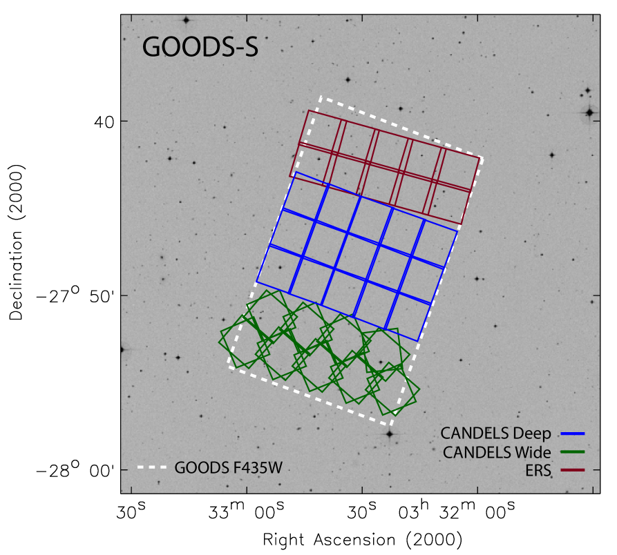
Figure 5.— A simplified footprint of the CANDELS observations in the GOODS-S field with WFC3/IR. The “Wide” portion of the CANDELS observations (green) and the pre-existing observations of the WFC3 ERS (brown) are reproduced faithfully. However the “Deep” portion of the field, represented here as a $3\times 5$ raster (blue), will in practice be observed across several epochs with slightly varying geometries. The individual epochs, as well as the footprints of the ACS parallel observations, are illustrated in Figures 11 and 12.

Additional multi-wavelength data in the GOODS-S field include $U$-band imaging obtained with VIMOS on the Very Large Telescope (VLT; Nonino et al. 2009), near-IR imaging in the $Y$ band with HAWK-I (Castellano et al. 2010a) and in the $J,H,$ and $K$-bands with ISAAC (Retzlaff et al. 2010) on the VLT, additional mid-IR imaging with Spitzer/IRAC (3.6–8.0 $\mu$m) from the SEDS program and Spitzer/MIPS (24 $\mu$m) from the Far-Infrared Deep Extragalactic Legacy survey (FIDEL; PI. M. Dickinson), submillimeter observations (870 $\mu$m) taken with LABOCA on the Apex telescope (Weiß et al. 2009), and radio imaging (1.4 and 4.8 GHz) from the Very Large Array (VLA; Kellermann et al. 2008). Furthermore, the field has been the subject of numerous spectroscopic surveys (e.g., Le Fèvre et al. 2004; Szokoly et al. 2004; Mignoli et al. 2005; Vanzella et al. 2005; Ravikumar et al. 2007; Cimatti et al. 2008; Popesso et al. 2009; Balestra et al. 2010; Silverman et al. 2010)

The CANDELS/Deep WFC3/IR observations in the GOODS-S field consist of a rectangular grid of $3\times 5$ WFC3/IR tiles ($\sim 6\farcm{8}\times 10^{\prime}$) that are oriented at a position angle of $70^{\circ}$ (East of North, see Fig. 5). The spacing intervals of each tile in the grid is designed to allow for maximal contiguous coverage in WFC3/IR without introducing gaps between tiles as a result of pointing errors. The orientation and location of the mosaic were chosen to overlap with the deepest portion of the existing Spitzer/IRAC imaging in the field, which, due to an overlap strip, peaks in the center of the GOODS region and is matched in orient and size with the CANDELS/Deep mosaic. When combined with the CANDELS/Wide observations in the field (see §5.2.4) and the imaging from the ERS program (ERS; Windhorst et al. 2011), the entire $10^{\prime}\times 16^{\prime}$ GOODS region will be imaged by WFC3/IR. An overview of the resulting WFC3/IR coverage in GOODS-S from all of these observations is shown in Figure 5. Due to the observational requirements of our various science programs, the actual observing strategy in GOODS-S is quite complex. This is described in §6.2.

5.1.2 The GOODS-North Field

The GOODS-N field is located near the northern Hubble Deep Field (Williams et al. 1996) and like its southern counterpart has been extensively observed by NASA’s Great Observatories. The field is centered at $\alpha$(J2000) = $12^{\rm h}$ $36^{\rm m}$ $55^{\rm s}$ and $\delta$(J2000) = $+62^{\circ}$ $14^{\prime}$ $15^{\prime\prime}$. The GOODS region of the field has been imaged in the optical with Hubble/ACS in the $B,V,i$, and $z$-bands as part of the GOODS Hubble Treasury Program. As in the GOODS-S field, this imaging covers a region $10^{\prime}\times 16^{\prime}$ in size and reaches $5\sigma$ depths of $B=28.0$, $V=28.0$, $i=27.5$, and $z=27.3$ mag (extended source). The field has also been imaged in the mid-IR (3.6–24 $\mu$m) as part of the GOODS Spitzer Legacy Program; this imaging reaches $5\sigma$ depths of 0.58, 0.55, 1.09, and 1.20 $\mu$Jy in the IRAC 3.6, 4.5, 5.8, and 8.0 $\mu$m bands, respectively, and 20 $\mu$Jy in the MIPS 24 $\mu$m band. Furthermore, the field has been targeted for deep Chandra observations that have a total integration time of 2 Ms (Alexander et al. 2003).

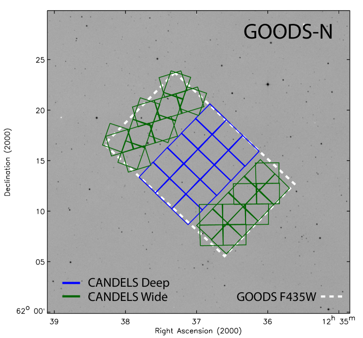
Figure 6.— A simplified footprint of the CANDELS observations in the GOODS-N field with WFC3/IR. The Wide portion of the CANDELS observations (green) is reproduced faithfully. However the Deep portion of the field, represented here as a $3\times 5$ raster (blue), will in reality will be observed across several epochs with slightly varying geometries. At the time of writing, the precise layout of each Deep epoch had not yet been determined. The ensemble will qualitatively resemble the progression in Figures 11 and 12.

Additional multi-wavelength data in the GOODS-N field include $U$-band imaging obtained with the MOSAIC camera on the KPNO Mayall 4m telescope (Capak et al. 2004), near-IR imaging in the $HK^{\prime}$-band taken with the QUIRC camera on the University of Hawaii 2.2 m telescope (Capak et al. 2004), additional mid-IR imaging with Spitzer/IRAC (3.6–8.0 $\mu$M) from the SEDS program and Spitzer/MIPS (24 $\mu$m) from the FIDEL survey and deep radio imaging (1.4 GHz) from the Very Large Array (VLA; Morrison et al. 2010). Furthermore, the field has been the subject of numerous spectroscopic surveys (e.g. Steidel et al. 2003; Wirth et al. 2004; Treu et al. 2005; Strolger et al. 2005; Reddy et al. 2006; Barger et al. 2008; Yoshikawa et al. 2010; Daddi et al. 2010; Cooper et al. 2011).

The CANDELS/Deep WFC3/IR observations in the GOODS-N field consist of a rectangular grid of $3\times 5$ WFC3/IR tiles ($\sim 6\farcm{8}\times 10^{\prime}$) that are oriented at a position angle of $45^{\circ}$ (East of North, see Fig. 6). As in GOODS-S, the orientation and location of the WFC3/IR mosaic were chosen to overlap with the deepest portion of the existing Spitzer/IRAC imaging in the field, which, due to an overlap strip, peaks in the center of the GOODS region and is matched in orient and size with the CANDELS/Deep mosaic. When combined with the CANDELS/Wide observations in the field (see §5.2.4), nearly the entire $10^{\prime}\times 16^{\prime}$ GOODS region will be imaged by WFC3/IR. An overview of the resulting WFC3/IR coverage in GOODS-N from all of these observations can be seen in Figure 6. The actual observing strategy in GOODS-N is quite complex and is described in §6.2.

5.2. CANDELS Wide Fields

The CANDELS/Wide fields consist of COSMOS, UDS, EGS and three smaller regions that bracket the CANDELS/Deep regions in GOODS-S and GOODS-N. In the three primary Wide fields (COSMOS, UDS, and EGS), we have chosen a long-thin geometry for the WFC3/IR observations in order to: i.) decorrelate clustering on the long axis, further reducing cosmic variance, ii.) maximize the area with overlapping and contemporaneous ACS/WFC parallel observations on top of the WFC3/IR mosaic, and iii.) increase the total lag over which correlation functions can be measured.

The precise location and orientation of the WFC3/IR mosaics on the sky were chosen based upon the location of ancillary data in each field and upon telescope scheduling constraints, namely roll angle visibility. The telescope’s roll angle determines the orientation of the WFC3/IR exposures and ultimately the placement of the ACS/WFC parallel exposures, which are offset from the prime exposures by roughly $6^{\prime}$. The visibility of a given roll angle is important because each CANDELS/Wide field is observed over two epochs separated by $\sim 50$ days in order to facilitate the search for high-$z$ SNe Ia. Therefore, to ensure a mosaic is repeated at the same orientation in each epoch, the observed roll angle must be accessible to the telescope for at least $\sim 50$ days and across both epochs of observation. This requirement severely limits the available observing windows. In the following subsections we discuss the existing data in each of the CANDELS/Wide fields and present our mosaic layouts.

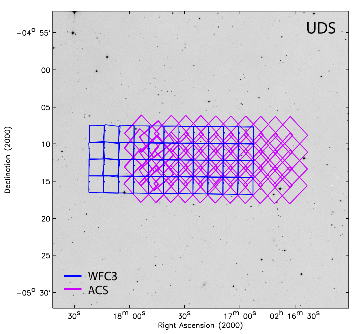
Figure 7.— Footprint of the CANDELS observations in the UDS field. The WFC3/IR prime exposures are shown in blue and the ACS/WFC parallel exposures shown in magenta.

5.2.1 The UDS Field

The UDS is the deepest component of the UKIRT Infrared Deep Sky Survey (UKIDSS; Lawrence et al. 2007). The full UDS field covers 0.8 sq degrees on the sky and is centered at $\alpha$(J2000) = $02^{\rm h}$ $17^{\rm m}$ $49^{\rm s}$ and $\delta$(J2000) = $-05^{\circ}$ $12^{\prime}$ $02^{\prime\prime}$. The field’s defining characteristic is deep J, H, and K imaging obtained with the UKIRT Wide Field Camera (WFCAM). When completed in 2012, this imaging will reach $5\sigma$ depths of $J=25.2,H=24.7$, and $K=25.0$ ($2^{\prime\prime}$-diameter aperture).

Optical imaging in the field consists of deep Subaru/SuprimeCam (Furusawa et al. 2008) observations in the $B,V,R,i$, and $z$-bands, which reach $3\sigma$ depths of $B=28.4,V=27.8,R=27.7,i=27.7$ and $z=26.6$ ($2^{\prime\prime}$-diameter aperture). Additional multi-wavelength data include $U$-band imaging obtained with MegaCam on the Canada-France-Hawaii Telescope (CFHT; P.I. O. Almaini), mid-IR (3.6–24 $\mu$m) observation taken with IRAC and MIPS on Spitzer as part of the Spitzer Ultra-Deep Survey (SpUDS; P.I. J. Dunlap) and the SEDS program, X-ray observations taken as part of the Subaru/XMM-Newton Deep Survey (SXDS; Sekiguchi et al. 2004); and deep radio imaging (1.4 GHz) from the VLA (Simpson et al. 2006). Furthermore, the UDSz program (P.I. O. Almaini) is carrying out a large redshift survey of the field using the VIMOS and FORS2 spectrographs on the VLT.

The CANDELS WFC3/IR observations in the UDS field consist of a rectangular grid of $4\times 11$ WFC3/IR tiles ($\sim 8\farcm{6}\times 23\farcm{8}$) that run East-to-West at a position angle of $-90^{\circ}$ (see Fig. 7). As with the CANDELS/Deep mosaics, the spacing intervals of each tile in the grid is designed to allow for maximal contiguous coverage in WFC3/IR without introducing gaps between tiles as a result of pointing errors. The exposures are all oriented so that the ACS/WFC parallels are offset along the long axis of the mosaic, thereby producing a similar-sized mosaic overlapping the bulk of the WFC3/IR mosaic except at its ends, where some tiles are covered only by WFC3/IR or by ACS/WFC and not by both.

The orientation and precise location of the mosaic was chosen with the following considerations in mind: i.) overlap with the SEDS IRAC imaging, ii.) alignment with the VIMOS spectroscopic observations, iii.) guide star availability, which ultimately shifted the entire mosaic $2^{\prime}$ to the west, and iv.) telescope roll angle visibility. The chosen position angle of $-90^{\circ}$ East-of-North fulfills the first and second requirements and it also corresponds to a telescope orient that can be held constant over both observing epochs. The layout of the mosaic and its position within the UDS field are shown in Figure 7.

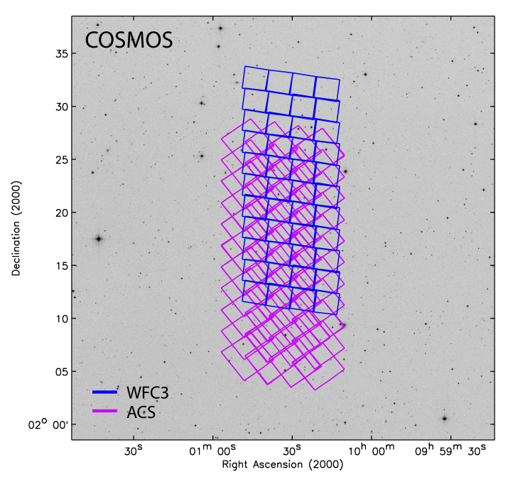
Figure 8.— Footprint of the CANDELS observations in the COSMOS field with WFC3/IR prime exposures shown in blue and ACS/WFC parallel exposures shown in magenta.

5.2.2 The COSMOS Field

The COSMOS field is a 2-degree region of sky surveyed with the Hubble/ACS in the F814W band by the COSMOS Treasury Program (Scoville et al. 2007; Koekemoer et al. 2007). The field is centered at $\alpha$(J2000) = $10^{\rm h}$ $00^{\rm m}$ $28^{\rm s}$ and $\delta$(J2000) = $+02^{\circ}$ $12^{\prime}$ $21^{\prime\prime}$ and has been extensively surveyed at a variety of wavelengths. Ground-based optical imaging of field includes deep Subaru/SuprimeCam observations in the $B,g^{\prime},V,r^{\prime},i^{\prime}$, and $z^{\prime}$-bands, which reach $3\sigma$ depths of $B=27.8,g^{\prime}=27.2,V=27.1,r^{\prime}=27.2,i^{\prime}=26.8$, and $z^{\prime}=25.9$ ($2^{\prime\prime}$-diameter aperture). In the near-IR, the Ultra-VISTA project (P.I. J. Dunlop) is imaging the central region of the field in the $Y$, $J$, $H$, and $K_{s}$ bands and when completed will reach $5\sigma$ depths of $\sim 25.5$ mag. The field is also being observed in five medium-band filters, which cover a wavelength range of 1–1.8$\mu$m using the NEWFIRM camera (P.I. P. van Dokkum; van Dokkum et al. 2009) on the Kitt Peak 4 m telescope.

Additional multi-wavelength data in the COSMOS field include X-ray observations with XMM-Newton (Hasinger et al. 2007), UV observations with GALEX (Zamojski et al. 2007), mid-IR (3.6–24 $\mu$m) observations with Spitzer (Sanders et al. 2007), submillimeter observations from the Caltech Submillimeter Observatory (CSO; Aguirre & Bolocam Galactic Plane Collaboration 2007), and radio observations with the VLA (Schinnerer et al. 2004, 2007). Furthermore, the zCOSMOS program (Lilly et al. 2007) is carrying out a large spectroscopic redshift survey of the field using the VIMOS spectrograph on the VLT, which will ultimately yield spectra for over 35,000 galaxies out to $z\approx 2.5$.

The CANDELS WFC3/IR observations in the COSMOS field consist of a rectangular grid of $4\times 11$ WFC3/IR tiles ($\sim 8\farcm{6}\times 23\farcm{8}$) that run North-to-South at a position angle of $180^{\circ}$ (see Fig. 8). The location of ancillary data in the COSMOS field constrained the location and orientation of the WFC3/IR mosaic to a greater degree than in the UDS field. The mosaic is positioned to lie within the overlap region of the mid-IR SEDS IRAC imaging, the medium-band NEWFIRM observations, and the near-IR Ultra-VISTA imaging. Unlike the UDS field, the telescope roll angle required to keep the WFC3/IR exposures aligned with the long axis of the mosaic is not visible throughout the two COSMOS observing epochs. To find a stable roll angle, we have rotated each WFC3/IR tile by $-8^{\circ}$ (East of North) relative to the mosaic’s position angle and used a slipped-lattice raster to maintain the North-South orientation for the overal mosaic. Due to the larger ACS/WFC footprint relative to WFC3/IR, the bulk of the ACS/WFC parallel exposures still overlap the WFC3/IR mosaic even with this rotation. The layout of the mosaic and its position within the COSMOS field are shown in Figure 8.

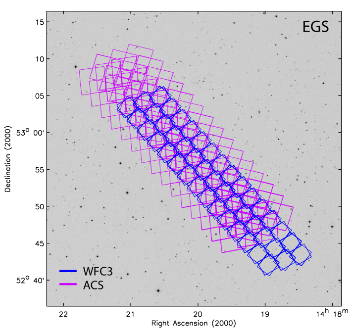
Figure 9.— Footprint of the CANDELS observations in the EGS field with WFC3/IR prime exposures shown in blue and ACS/WFC parallel exposures shown in magenta. Just over half of the area was observed in HST Cycle 18, while the remainder will be observed in HST Cycle 20. The two halves are shown independently in Figure 10.

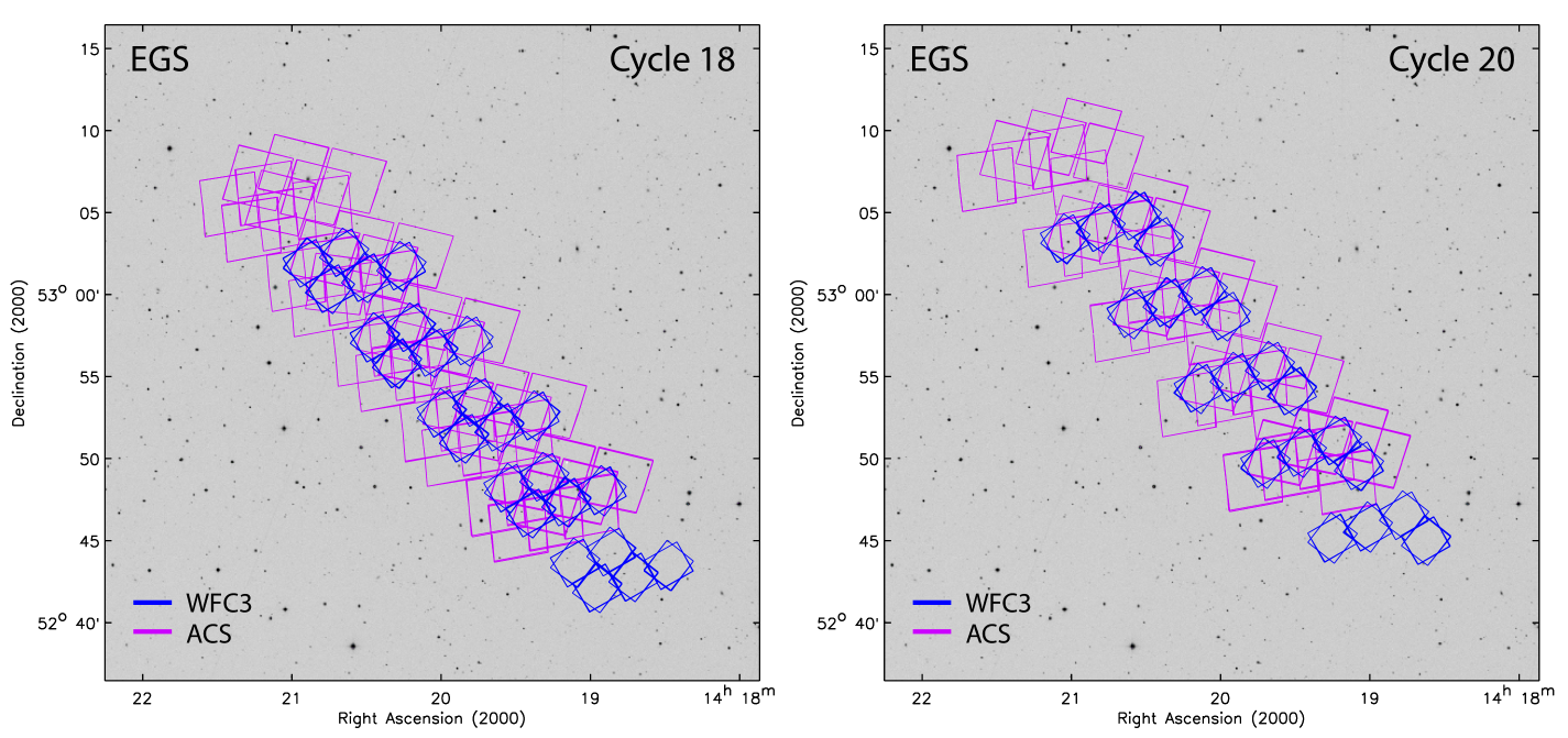
Figure 10.— Footprints of the two CANDELS campaigns in the EGS field. Slightly over half the total area was observed in HST Cycle 18 (left), while the remainder will be observed in HST Cycle 20 (right). The WFC3/IR prime exposures are shown in blue, and the ACS/WFC parallel exposures are shown in magenta.

5.2.3 The EGS Field

The EGS is a region of sky that has been extensively studied by the All-wavelength Extended Groth strip International Survey (AEGIS; Davis et al. 2007). The field is centered at $\alpha$(J2000) = $14^{\rm h}$ $17^{\rm m}$ $00^{\rm s}$ and $\delta$(J2000) = $+52^{\circ}$ $30^{\prime}$ $00^{\prime\prime}$ and owes its name to an early Hubble/WFPC2 survey carried out by the WFPC team (Rhodes et al. 2000). More recently the field has been imaged with ACS/WFC in the F606W and F814W bands (P.I. M. Davis), reaching $5\sigma$ depths of 28.75 and 28.1 mag, respectively. Ground-based optical imaging of the field includes deep CFHT/MegaCam observations in the $u^{*},g^{\prime},r^{\prime},i^{\prime}$, and $z^{\prime}$-bands, which reach $5\sigma$ depths of $u^{*}=28.3$, $g^{\prime}\approx 27.5$, $r^{\prime}$, $i^{\prime}=26.4$, and $z^{\prime}=26.4$ mag (Gwyn 2008). The field is also being observed in five medium-band filters, which cover a wavelength range of $1-1.8\mu$m, using the NEWFIRM camera (P.I. P. van Dokkum; van Dokkum et al. 2009) on the Kitt Peak 4 m telescope.

Additional multi-wavelength data in the EGS include $B,R,$ and $I$-band imaging obtained with the CFHT 12K mosaic camera (Cuillandre et al. 2001; Coil et al. 2004), near-IR imaging in the $J$ and $K_{s}$ bands taken with Wide-Field Infrared Camera (WIRC) on the Palomar 5m telescope, mid-IR (3.6–24 $\mu$m) observations taken with IRAC and MIPS on Spitzer as part of the GTO program 8 and the SEDS program, far-IR ($70\mu$m) observations taken with Spitzer/MIPS as part of the FIDEL survey, X-ray observations taken with Chandra (Laird et al. 2009), UV observations taken with GALEX, and radio imaging (1.4 and 4.8 GHz) from the VLA (Willner et al. 2006; Ivison et al. 2007). Furthermore, the DEEP2 and DEEP3 programs (Davis et al. 2003, , Newman et al. 2011, in prep.) have carried out an extensive spectroscopic survey of the EGS using the Deep Imaging Multi-Object Spectrograph (DEIMOS; Faber et al. 2003) on the Keck II 10m telescope.

The CANDELS WFC3/IR observations in the EGS consist of a rectangular grid of $3\times 15$ WFC3/IR tiles ($\sim 6\farcm{7}\times 30\farcm{6}$) that is oriented at a position angle of $42^{\circ}$ (see Fig. 9). As in the COSMOS field, the location of ancillary data in the EGS heavily constrains the location and orientation of the WFC3/IR mosaic. The existing Hubble/ACS imaging in the field is roughly $10^{\prime}$ wide and is oriented at a position angle of $40^{\circ}$. The CANDELS mosaic is positioned to lie within these existing data and to maximize overlap with the mid-IR SEDS imaging, the far-IR FIDEL imaging, and the deepest portion of the Chandra observations in the field. The EGS also has the strictest scheduling constraints; there exists no roll angle for the EGS that can be held fixed throughout both observing epochs. Therefore, we have devised a layout in which each WFC3/IR tile is rotated $+11^{\circ}$ (East-of-North) during the first imaging epoch and $-11^{\circ}$ during the second. This results in a larger portion of the ACS/WFC parallel exposures falling outside the WFC3/IR mosaic than in the UDS and COSMOS fields, but due to the larger ACS/WFC footprint, the mosaic remains nearly entirely covered by the ACS/WFC optical imaging. The layout of the mosaic and its position within the EGS are shown in Figure 9.

5.2.4 The GOODS South and North Fields

The Wide-depth CANDELS WFC3/IR observations in the GOODS-S and GOODS-N fields consist of three regions (one in GOODS-S and two in GOODS-N) that flank the CANDELS/Deep regions in each field. The location and orientation of these regions are shown in Figures 5 and 6. In GOODS-S this Wide-depth “flanking field” contains a total of nine WFC3/IR tiles oriented to place most of their ACS/WFC parallel exposures into the CANDELS/Deep region. In GOODS-N, the two flanking fields contain eight WFC3/IR tiles each and are again oriented such that their ACS/WFC parallel exposures fall within the CANDELS/Deep region. A second flanking field in GOODS-S is effectively provided by the existing WFC3/IR observations from the ERS program, which are adjacent and to the North of the CANDELS/Deep region. When combined with the CANDELS/Deep observations and the ERS imaging, these flanking fields will provide WFC3/IR coverage over nearly the entire $10^{\prime}\times 16^{\prime}$ extents of the two GOODS regions.

5.3. Mitigating Cosmic Variance

Table 5Cosmic Variance Estimates

CANDELS Field	Area	$CV_{z=2}$	$CV_{z=7}$
GOODS-North (Deep)	$6\farcm{8}\times 10\farcm{0}$	0.476 $(b/5.5)$	0.578 $(b/15)$
GOODS-South (Deep)	$6\farcm{8}\times 10\farcm{0}$	0.476 $(b/5.5)$	0.578 $(b/15)$
GOODS-North (Wide)	$9\farcm{7}\times 16\farcm{4}$	0.404 $(b/5.5)$	0.469 $(b/15)$
GOODS-South (Wide)	$9\farcm{9}\times 14\farcm{9}$	0.412 $(b/5.5)$	0.481 $(b/15)$
COSMOS	$9\farcm{0}\times 22\farcm{4}$	0.375 $(b/5.5)$	0.429 $(b/15)$
UDS	$9\farcm{4}\times 22\farcm{0}$	0.354 $(b/5.5)$	0.405 $(b/15)$
EGS	$6\farcm{4}\times 30\farcm{5}$	0.375 $(b/5.5)$	0.430 $(b/15)$
Deep Total	0.038 sq deg	0.337 $(b/5.5)$	0.409 $(b/15)$
Wide Total	0.290 sq deg	0.171 $(b/5.5)$	0.197 $(b/15)$

Note. — A single $32\farcm{4}\times 32\farcm{4}$ field covering the same total area as the Wide program results in $CV_{z=2}=0.250$ $(b/5.5)$ and $CV_{z=7}=0.259$ $(b/15)$.

The primary reason CANDELS has focused on five different fields, rather than one or two, is to minimize the impact of the variation in the mean density of matter (and hence also of galaxies of some class) from one region to another, commonly referred to as “sample variance” or “cosmic variance”. This effect can be comparable to or larger than Poisson variance, and hence will have large impact on the determination of the abundance of a class of objects (e.g., the normalization of the LF). The impact of cosmic variance is most simply reduced by surveying a larger volume of the Universe; however, that is expensive in terms of telescope time. Given a fixed survey area, it will be minimized by dividing that area amongst multiple widely-separated fields, as the density fluctuations in those fields will be statistically independent; for a single field, cosmic variance is reduced if the field has a long, narrow geometry as opposed to a square one, as that maximizes the typical distance between objects and ensures greater independence between different portions of the field (i.e., samples more quasi-independent volumes; cf. Newman & Davis 2002). Cosmic variance is also a driver for the geometry of individual CANDELS/Wide fields; we have made them as elongated as possible while maintaining overlap with other relevant datasets and retaining the ability to measure correlation functions accurately.

We have used the public QUICKCV code (Newman & Davis 2002) to predict the impact of cosmic variance for representative CANDELS samples, and compared to other simple scenarios. The fractional uncertainty in the abundance of some class of object will scale as its linear bias, $b$. We consider two fiducial scenarios: counting the abundance of galaxies at $z=1.75-2.25$ with stellar mass $10^{11}-10^{11.5}$, using the results of Faber et al. (2003) to predict their bias, or counting the abundance of a sample of galaxies at $z=6.5-7.5$ with the same clustering properties (in comoving coordinates) as the $z=2$ sample, corresponding to a bias of 15 compared to dark matter at the same redshift. These samples represent approximate upper limits to the impact of cosmic variance; any more biased sample at the same redshifts should be extremely rare and dominated by Poisson uncertainties. The results of these calculations are given in Table 5.

Hence, the net cosmic variance for the CANDELS/Wide survey should be roughly $17\%$ $(b/5.5)$ for a sample at $z=1.75-2.25$, or $20\%$ $(b/15)$ for a sample at $z=6.5-7.5$. Even for more typical galaxies with a large-scale structure bias one-third as large as our fiducial samples, cosmic variance should contribute significantly to errors so long as the sample contains more than $\sim 100$ objects over the CANDELS survey. These numbers are significant, but compare very favorably to a square (or nearly so) survey that covers a single field, such as the COSMOS survey. A single-field survey of the same total area as CANDELS (i.e. a $32.4\arcmin\times 32.4\arcmin$ field) would have errors from cosmic variance of 25% $(b/5.5)$ at $z\approx 2$ or 26% $(b/15)$ at $z\approx 7$, almost 50% larger than for our chosen geometry. To match the cosmic variance uncertainties from a CANDELS sample, a single field would have to be $55.5\arcmin\times 55.5\arcmin$ across, corresponding to an area (and hence time to survey) 2.94$\times$ larger than CANDELS.

Figure 11.— Footprints of the first eight epochs of CANDELS observations in the GOODS-S field with WFC3/IR and ACS/WFC. The blue and orange outlines are individual WFC3/IR pointings in the $J/H$ and $Y$ filters, respectively. The corresponding ACS/WFC parallels shown in magenta, red, or green according to the ACS filter selection. The black box is the fiducial CANDELS/Deep region, to guide the eye. At the top of each epoch is shown the pre-existing exposure map from the WFC3 ERS observations in this field (purple). These ERS observations are intermediate in depth between the CANDELS Deep and Wide components.

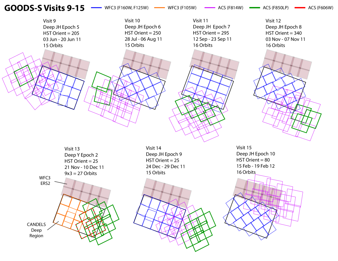
Figure 12.— Footprints of the last seven epochs of CANDELS observations in the GOODS-S field with WFC3/IR and ACS/WFC. See Figure 11 for a description.

6. Observing Strategy

The CANDELS observing strategy is very tightly constrained by several competing science goals and by the scheduling limitations of HST. Because CANDELS is an HST Multi-cycle Treasury Program, it will be observed over the three years of HST Cycles 18, 19, and 20. At the time of writing, only the Cycle 18 and 19 observations have officially been planned through to the so-called “Phase II” stage. In this section, we describe the observing strategy in detail, with particular attention to the constraints that have shaped our decisions.

The Cycle 18 observations include both epochs of the full UDS field, both epochs of the first half of the EGS field (see Figs. 9 and 10), and several epochs of the GOODS-S field. The latest specifics of these observations may be obtained from the STScI website as Programs 12060 (non-SN-searched GOODS-S), 12061 and 12062 (SN-searched GOODS-S), 12063 (first-half EGS), and 12064 (UDS). Program 12062 includes observations that extend into Cycle 19. The COSMOS and GOODS-N observations for Cycle 19 were planned through the Phase II stage in mid-2011. The COSMOS observations have been assigned Program 12440, and the GOODS-N observations have been assigned Programs 12442 (non-SN-searched GOODS-N), 12443, 12444, and 12445 (successive thirds of the SN-searched GOODS-N). The Cycle 20 observations will comprise the latter portion of GOODS-N (Programs 12444, 12445, and roughly half of 12442) and the second-half of EGS (Program 12063), whose specifics will have been largely pre-determined by our earlier observations of these fields in Cycles 19 and 18, respectively. The scheduling constraints upon all CANDELS fields are already sufficiently tight that we can describe the expected layouts and timings with reasonable certainty.

As in the previous section, the detailed description of the observing strategy is best split between the CANDELS/Wide fields and the CANDELS/Deep fields.

6.1. Wide-Field Strategy

In the CANDELS/Wide fields, the goal is to cover a large area at two-orbit depth while maintaining the ability to search for SNe in the near-IR with WFC3.

The SN search requires that we repeatedly observe a given location in WFC3 F125W and F160W with time separation(s) of $\sim 52$ days. Given that each of the CANDELS/Wide areas comprises dozens of WFC3/IR fields of view, the minimum efficient dwell time is one full orbit per pointing per epoch. The minimum SN search is a pair of epochs separated by 52 d, which gives us a total of two-orbit depth with WFC3/IR in the Wide fields.

It is crucial that we have nearly contemporaneous observations in an optical filter to discriminate the type (and the photometric redshift) of a WFC3-detected SN. We have therefore adopted a long and narrow geometry for the CANDELS/Wide fields, such that ACS parallel observations will overlap the majority of the WFC3/IR coverage (see Figs. 7, 8, and 9).

For the CANDELS UDS, our desired long-axis position angle (East–West) fortuitously corresponds to a telescope orientation that can be held constant across both epochs. The same is nearly true for the COSMOS field, where the desired North–South alignment is within several degrees of a stable HST orientation and permits a slipped-lattice WFC3/IR raster (see Fig. 8). The difference between this arrangement and an orthogonal raster is small enough that ACS parallel fields still overlap the WFC3/IR footprint, as desired for the SN search.

For the EGS field, there is no HST orientation near our desired Northeast–Southwest alignment that can be held for the entire duration of observing the full field at both epochs. We therefore observe half the field in one campaign (both epochs) in Cycle 18, and the other half in another campaign (also both epochs) in Cycle 20. Furthermore, in each EGS campaign the first epoch is observed at a position angle $11\arcdeg$ counterclockwise of the desired alignment; the second epoch at $11\arcdeg$ clockwise of the desired alignment. The rotations are necessary because of our inability to maintain a fixed roll angle of HST across the $\sim 8.5$ weeks spanned by the two epochs. As with the COSMOS field, the displacements away from the EGS tiling orientation are not so large that the ACS parallels miss the WFC3/IR footprint (see Fig. 9).

Some care must be taken in dividing the full EGS tiling so that WFC3/IR and ACS are overlapping in the respective halves. It is unavoidable, when dividing the EGS tilings into two campaigns, that there will be less contemporaneous overlap of WFC3/IR and ACS than if we could observe the entire field in a single campaign. Our solution, which we believe minimizes this overlap loss, is the tiling scheme shown in Figure 10. The key element is to divide the mosaic into bands separated by $\sim 6\arcmin$, matching the offset between the contemporaneous fields of view of WFC3/IR and ACS.

Because of the large offset between these fields of view, the first three rows of WFC3/IR pointings along the long axis of the CANDELS/Wide fields will inevitably lack ACS parallel coverage. As a corollary, the ACS parallel coverage of the CANDELS/Wide fields will extend several arcminutes past the WFC3/IR footprint at the other end of the long axis. Lacking parallel ACS coverage in the first three rows of WFC3/IR pointings, we have elected to use WFC3/UVIS in order to obtain the contemporaneous optical coverage needed for SN discrimination. This added UVIS exposure, which can be taken in the “white-light” filter F350LP for maximum throughput, foreshortens the WFC3/IR exposure depth in these first three rows by 410 s per epoch. The UDS and COSMOS fields, which are $4\times 11$ tilings, therefore have 12 tiles with reduced IR exposure. The EGS field, which is a $3\times 15$ tiling, has nine tiles with reduced IR exposure.

To even sensitivity in AB magnitudes, we seek to obtain a 2:1 ratio of exposure time in the WFC3/IR filters F160W and F125W. We also desire four WFC3/IR exposures per epoch, using the same filter and exposure combinations in each epoch, to make a well-dithered mosaic for SN detection (see Koekemoer et al. 2011 for details). We therefore strive at each WFC3/IR pointing to obtain two long F160W exposures and two short F125W exposures. Pointings that require an additional WFC3/UVIS exposure (see above) will have an F160W:F125W exposure ratio closer to 1:1. This variation in exposure ratio is necessary because the F125W exposures are already near the minimum duration to accommodate the HST buffer dump of the prior ACS (and sometimes WFC3) exposure in parallel with the current exposure. Shorter F125W exposure time would trigger a serial (rather than parallel) buffer dump, in effect precluding the exposure.

For the ACS parallel exposures in the CANDELS/Wide fields, the need for maximally efficient discovery of high-$z$ dropout galaxies pushes toward a 2:1 ratio of exposure in the filters F814W and F606W. In the EGS and COSMOS fields, which contain legacy ACS data in these filters (see §5.2 for details), the goal is to adjust the CANDELS exposure ratios such that the cumulative exposure is 2:1 for F814W:F606W. Because the ACS field of view is very nearly twice that of WFC3/IR, our abutting WFC3/IR raster results in most of the ACS parallel footprint having double the coverage, or effectively two-orbit depth per epoch. The two epochs thus provide a total of four-orbit depth of ACS parallel coverage divided between F814W and F606W.

In the CANDELS UDS field, where there exists no prior full-field coverage with ACS, each epoch yields 2/3-orbit F606W and 4/3-orbit F814W. In the CANDELS EGS field, which contains prior F606W and F814W images totaling one-orbit depth apiece (Program 10134; P.I.: M. Davis), we take no F606W data in the first epoch, and split between F606W and F814W in the second epoch, to achieve approximate 2- and 4-orbit total depth in F606W and F814W. In the CANDELS COSMOS field, where there exists one orbit of F814W, we allocate the new ACS parallels in a 1:2 ratio of F606W:F814W in the first epoch, and a 2:1 ratio in the second epoch, resulting in a total depth of 2- and 3-orbits in F606W and F814W.

Figures 13a-e show the planned exposure maps for the CANDELS UDS field in the filters F350LP (WFC3/UVIS), F606W (ACS/WFC), F814W (ACS/WFC), F125W (WFC3/IR), and F160W (WFC3/IR).

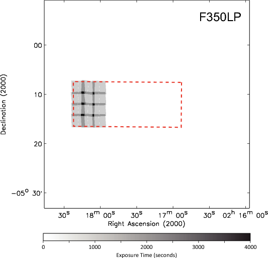
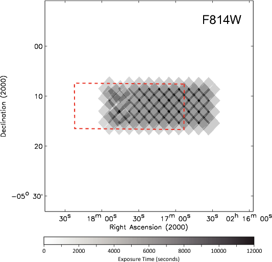
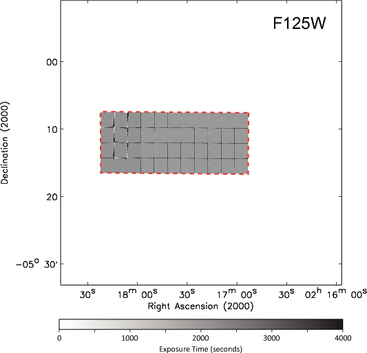
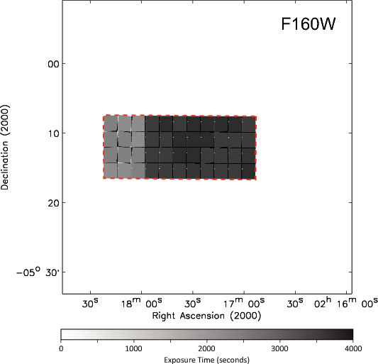
Figure 13.— Exposure maps for the CANDELS UDS region. The ACS exposure maps (F606W and F814W) are on a linear stretch from 0 to 12 ks. The WFC3 exposure maps (F350LP, F125W, and F160W) are on a linear stretch from 0 to 4 ks. The dotted red line indicates the bounds of the F160W coverage.

Figures 14a-e show the planned exposure maps for the CANDELS EGS field in the filters F350LP (WFC3/UVIS), F606W (ACS/WFC), F814W (ACS/WFC), F125W (WFC3/IR), and F160W (WFC3/IR). The ACS exposure maps include the legacy EGS imaging from Program 10134.

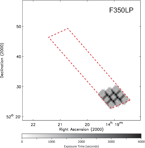
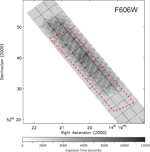
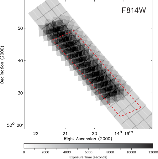
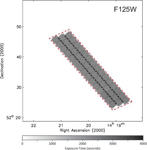
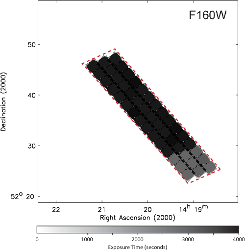
Figure 14.— Exposure maps for the CANDELS EGS region, including legacy ACS/WFC exposures. The ACS exposure maps (F606W and F814W) are on a linear stretch from 0 to 12 ks. The WFC3 exposure maps (F350LP, F125W, and F160W) are on a linear stretch from 0 to 4 ks. The dotted red line indicates the bounds of the F160W coverage.

Figures 15a-e show the planned exposure maps for the CANDELS COSMOS field in the filters F350LP (WFC3/UVIS), F606W (ACS/WFC), F814W (ACS/WFC), F125W (WFC3/IR), and F160W (WFC3/IR). The ACS exposure maps include the legacy COSMOS imaging from Programs 9822 and 10092.

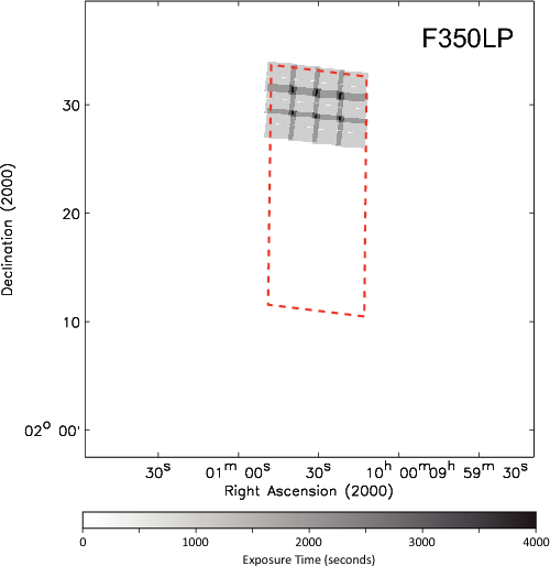
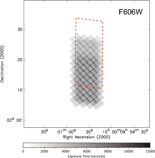
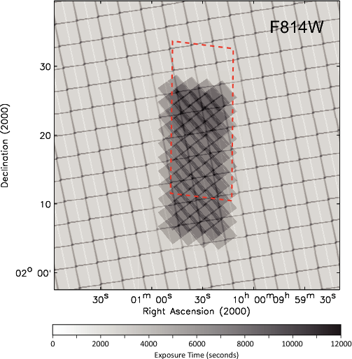
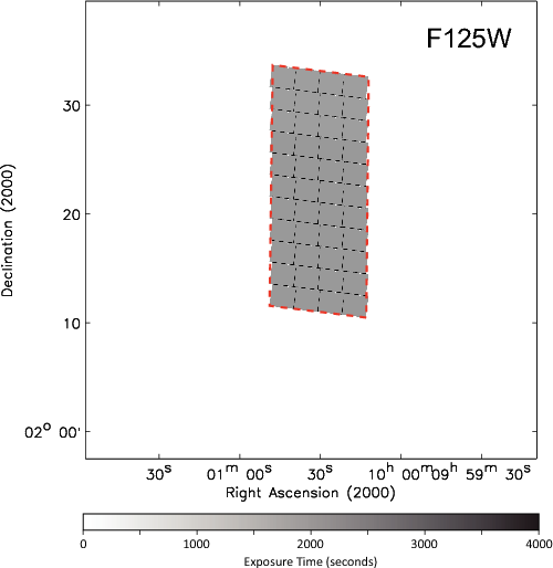
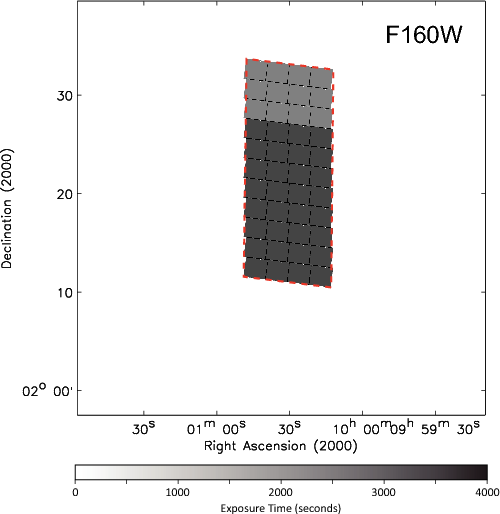
Figure 15.— Exposure maps for the CANDELS COSMOS region, including legacy ACS/WFC exposures. The ACS exposure maps (F606W and F814W) are on a linear stretch from 0 to 12 ks. The WFC3 exposure maps (F350LP, F125W, and F160W) are on a linear stretch from 0 to 4 ks. The dotted red line indicates the bounds of the F160W coverage.

Figures 16a-c show the curves of area versus exposure depth for each of the ACS and WFC3 filters that will comprise CANDELS UDS, EGS, and COSMOS fields. Each of these area vs. depth plots only consider the area within the footprint of the CANDELS F160W images and includes the legacy ACS data.

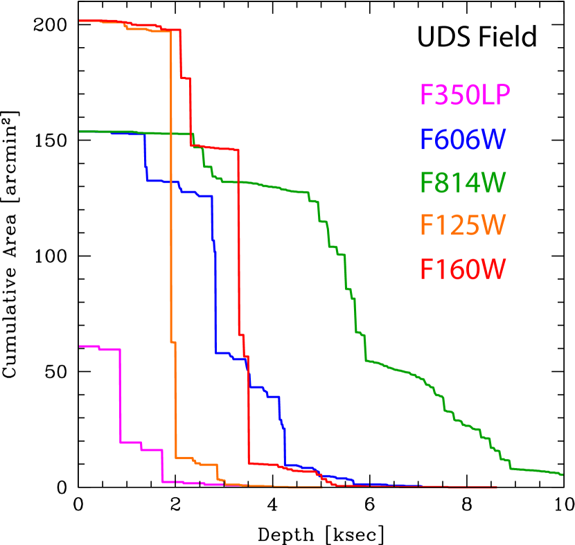
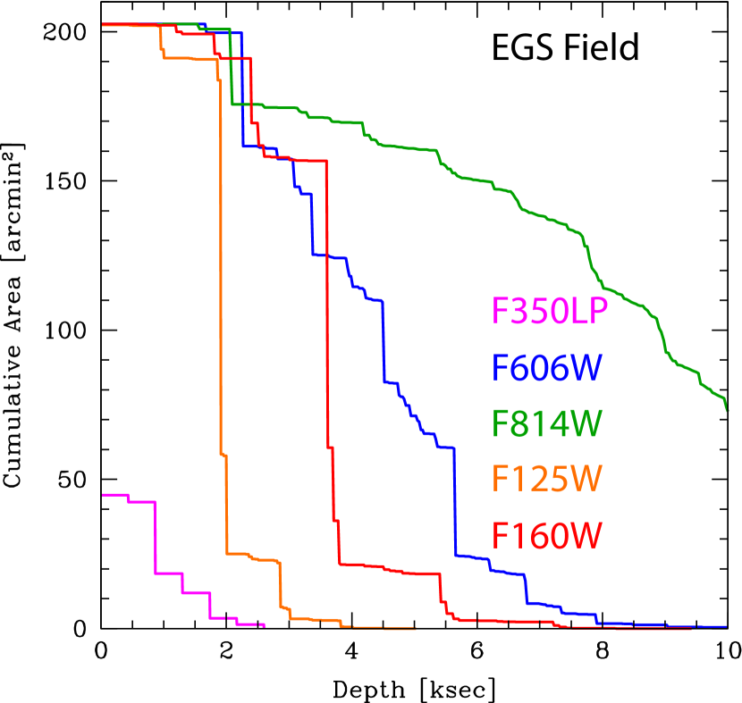
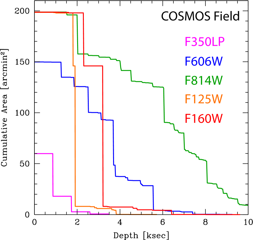
Figure 16.— Cumulative area vs. depth profiles of the CANDELS/Wide fields, including legacy ACS/WFC exposures. The areas are limited to the footprints of the CANDELS F160W images in each field.

6.2. Deep-field Strategy

In the CANDELS/Deep fields, the primary observational goal is to obtain WFC3 and ACS imaging across moderately large regions that are substantially deeper than the CANDELS/Wide fields. Unlike the CANDELS/Wide fields, completed in two epochs, the CANDELS/Deep fields are imaged for ten SN-searched epochs in F125W and F160W, as well as additional epochs in F105W ($Y$-band) that are not SN-searched. The target is 10 ks total exposure in these three WFC3 filters.

To enable the robust identification of extreme-redshift galaxies in the CANDELS/Deep fields, we also design the observing plan to attain at least 25 ks of ACS F814W exposure across the entire area covered by the deep WFC3/IR images. The majority of this F814W depth is obtained from ACS parallel exposures during the $Y$-band epochs (e.g., Fig. 11, Visit 8; Fig. 12, Visit 13).

Our orbit allocation permits us to cover roughly 40% of the $\sim 10\arcmin\times 16\arcmin$ GOODS ACS regions for CANDELS/Deep. We have chosen a placement that contains the zones of deepest GOODS Spitzer coverage: $>45$ hr exposure time with IRAC (3.6$\mu$m–8$\mu$m). Recognizing that the remainder of the GOODS ACS regions are still extremely valuable for moderate-redshift science in conjunction with WFC3, we image the GOODS areas outside the CANDELS/Deep fields with a two-epoch observing strategy similar to the CANDELS/Wide fields above. Because these flanking fields have superior multicolor ACS imaging as compared with the CANDELS/Wide fields, we also image them with F105W ($Y$-band) to complete the HST wavelength coverage of the entire GOODS area from $B$-band (F435W) to $H$-band (F160W). Judicious scheduling of these CANDELS/Deep flanking fields allows us to place additional ACS parallel F814W exposures into the CANDELS/Deep fields (e.g., Fig. 11, Visits 3, 5, and 7).

In the CANDELS GOODS-S field, we have designed our observing strategy to be complementary to the existing observations by the WFC3 ERS. Those ERS observations match quite closely what we would desire for a northwest flanking field of CANDELS/Deep, and to depths in F125W and F160W that actually exceed the CANDELS/Wide target. We therefore observe only the southeast flanking field in GOODS-S. We note that the ERS observations in $Y$-band were taken with F098M rather than F105W. We choose F105W in the GOODS-S flanking field for consistency with the CANDELS/Deep fields, the GOODS-N flanking fields, and deep F105W imaging in GOODS-S from the HUDF09 program. We note that the ERS F098M exposure time is roughly twice that of the flanking-field F105W, so the $Y$-band sensitivity across ERS will be at least that of the flanking fields despite the narrower bandpass.

In CANDELS GOODS-N, where there exists no ancillary WFC3 imaging, we will observe both flanking fields identically in F105W, F125W, and F160W. During the GOODS-N Deep epochs, we will also take advantage of CVZ opportunities to image the Deep region in UV with WFC3/UVIS (F275W and F336W). Because these UV exposures will be read-noise limited, we have chosen the $2\times 2$-binned mode. This binning yields $\sim 0.5$ mag additional sensitivity at only modest expense in angular resolution for the drizzled UV mosaics, given our sub-pixel dithering. To facilitate the selection of Lyman-break drop-outs at $z\approx 2$ and to increase the sensitivity to LyC radiation at $z\approx 2.5$ (see §3.4), the goal is a 2:1 ratio of exposure time for F275W:F336W. We expect extended-source sensitivities of $\sim 27.9$ and $\sim 27.7$ mag in F275W and F336W, respectively. Caveats include uncertainties in the durations of the narrow windows for CVZ scheduling, and in the degradation of the UVIS detectors’ charge transfer efficiency — important for these low-background UV exposures.

During the ten epochs of the CANDELS/Deep campaigns, the ACS parallel observations pivot with the orientation of HST throughout the year, sometimes landing outside the larger GOODS ACS box entirely (see Figs. 11 and 12). In GOODS-S, this extended region has shallow ACS coverage in F606W and F850LP from the GEMS program. Because the area coverage of ACS/WFC is $\sim 2$ times that of WFC3/IR, we have approximately two-orbit depth in ACS parallel coverage at each Deep epoch. We have developed a strategy for filter selection among these far-flung ACS parallels according to the decision tree:

• If the ACS field intersects the CANDELS/Deep: first priority is to exceed 25 ks depth in F814W; second priority is one orbit of F850LP for variability study (with GOODS and PANS); third priority is additional F606W or F814W as appropriate to reach a 1:2 ratio of exposure in those two filters.

• If the ACS field intersects the CANDELS/Deep flanking fields: first priority is to exceed two orbits of F814W (the F606W depth across the GOODS fields exceeds 3 orbits); second priority is one orbit of F850LP for variability study (with GOODS and PANS); third priority is additional F606W or F814W as appropriate to reach a 1:2 ratio of exposure in those two filters.

• If the ACS field is entirely outside the CANDELS+ERS WFC3: first priority in GOODS-S is one orbit of F850LP for variability study (with GEMS); otherwise we allocate between F606W and F814W as appropriate to reach a 1:2 ratio of exposure in those two filters. The full coverage of our CANDELS GOODS-S ACS parallels includes at least 1-orbit-depth F606W from the GEMS program. There is very little ancillary ACS imaging in F606W, F814W, or F850LP just outside the footprint of GOODS-N.

Because the CANDELS GOODS epochs individually cover compact regions with WFC3, we are unable to use the ACS parallels for contemporaneous optical discrimination of distant SNe as we can with the CANDELS/Wide fields. Therefore, all of our CANDELS GOODS SN search epochs include a short WFC3/UVIS F350LP exposure at each pointing. This configuration is nearly identical to that used for the small portions of the CANDELS/Wide fields lacking ACS parallel coverage. The $Y$-band epochs, which are not used for SN Ia searching, are taken without F350LP exposures. In the Deep regions, the F105W is also obtained with multi-orbit visits, reducing HST guide-star acquisition overhead. Both situations result in more F105W exposure per orbit than we achieve for F125W and F160W. Our three-orbit visits for the Deep F105W obtain nearly as much exposure time as F125W and F160W attain in their ten shared-orbit visits.

Figures 17a-f show the planned exposure maps for the CANDELS GOODS-S field in the bluer filters: F275W (WFC3/UVIS), F336W (WFC3/UVIS), F350LP (WFC3/UVIS), F435W (ACS/WFC), F606W (ACS/WFC), and F775W (ACS/WFC). Figures 18a-f show the planned exposure maps for the CANDELS GOODS-S field in the redder filters: F814W (ACS/WFC3), F850LP (ACS/WFC), F098M (WFC3/IR), F105W (WFC3/IR), F125W (WFC3/IR), and F160W (WFC3/IR). The exposure maps include all available ACS and WFC3 legacy imaging in this region matching the combined GOODS and CANDELS filter sets. In particular, the F275W and F336W exposures come entirely from the ERS (Program 11359) and are shown because CANDELS will also be obtaining exposures in these filters in the GOODS-N field. The F098M imaging in the ERS is also shown, as this will be used as a proxy for the F105W imaging that CANDELS is employing elsewhere in the field. We also note that the F775W data is entirely from legacy observations, principally GOODS and PANS.

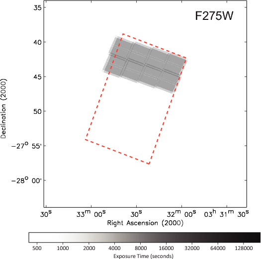
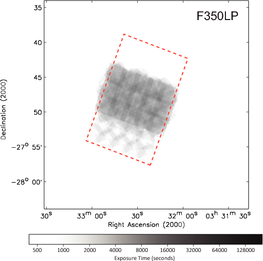
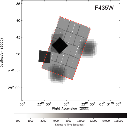
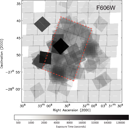
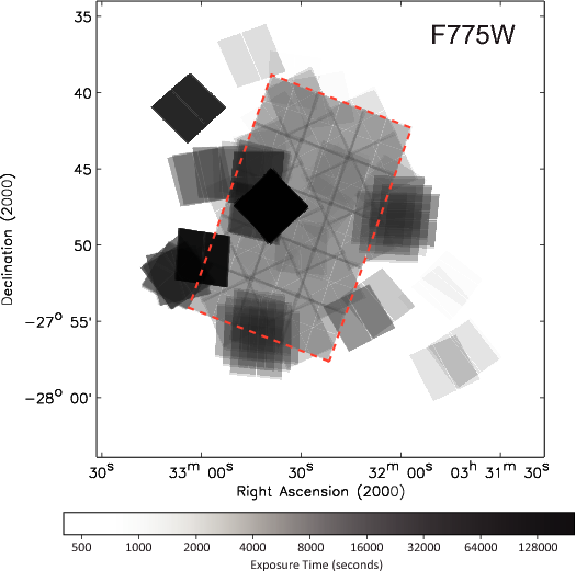
Figure 17.— Exposure maps for the bluer filters of the CANDELS GOODS-S region, including legacy ACS and WFC3 exposures. All exposure maps are plotted with a logarithmic stretch from 0.4 to 200 ks. The small extreme-depth portions of the exposure maps are the HUDF and its parallel fields. The dotted red line indicates the fiducial GOODS ACS boundary.

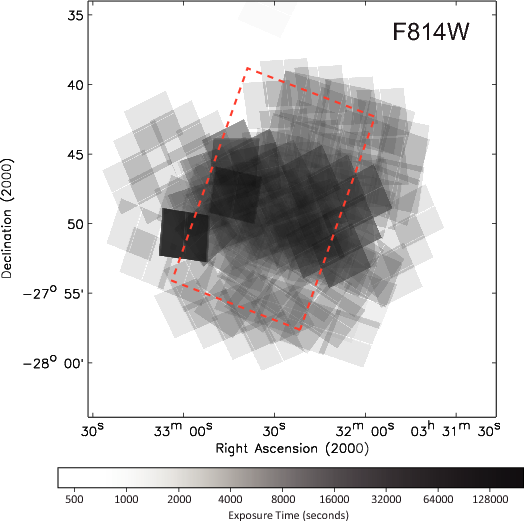
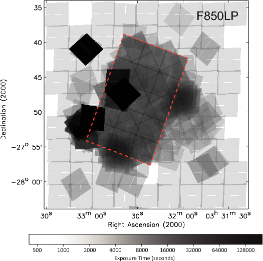
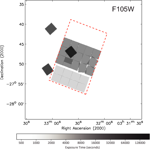
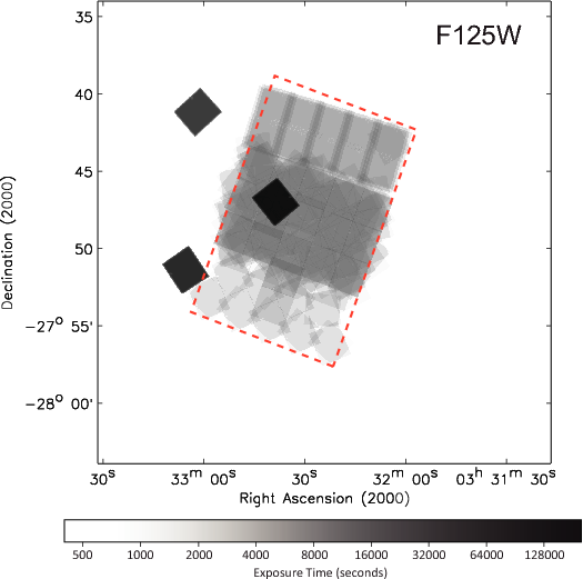
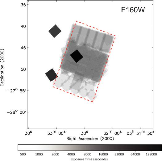
Figure 18.— Exposure maps for the redder filters of the CANDELS GOODS-S region, including legacy ACS and WFC3 exposures. All exposure maps are plotted with a logarithmic stretch from 0.4 to 200 ks. The small extreme-depth portions of the exposure maps are the HUDF and its parallel fields. The dotted red line indicates the fiducial GOODS ACS boundary.

Figures 19a,b show the curves of area versus exposure depth for each of the ACS and WFC3 filters that will comprise the CANDELS GOODS-S field. Each of these area vs. depth plots considers only the area within the footprint that is the union of the ERS and the CANDELS images but does include all legacy ACS and WFC3 data. Note that the F098M and F105W coverages are almost entirely non-overlapping, and thus their area-depth curves may be approximately stacked to represent the $Y$-band counterpart to the available $J$ and $H$ images.

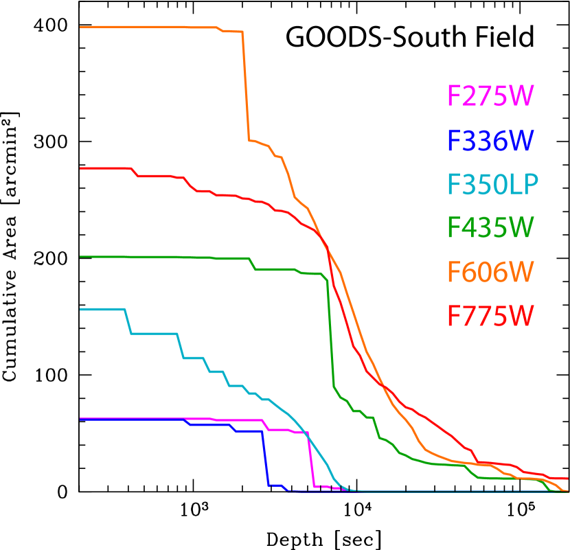
Figure 19.— Cumulative area vs. depth profiles of the CANDELS GOODS-S field, including legacy ACS and WFC3 exposures. The areas are limited to the footprint covered by the union of ERS and CANDELS images.

Figures 20a-f show the planned exposure maps for the CANDELS GOODS-N field in the bluer filters: F275W (WFC3/UVIS), F336W (WFC3/UVIS), F350LP (WFC3/UVIS), F435W (ACS/WFC), F606W (ACS/WFC), and F775W (ACS/WFC). We note that the original GOODS+PANS F775W coverage in GOODS-N has been substantially augmented by the ACS parallel exposures of the large WFC3/IR grism survey by Weiner et al. (Program 11600). This additional F775W imaging is reflected in Figure 20f and in the F775W area vs. depth curve to follow. Figures 21a-e show the planned exposure maps for the CANDELS GOODS-N field in the redder filters: F814W (ACS/WFC3), F850LP (ACS/WFC), F105W (WFC3/IR), F125W (WFC3/IR), and F160W (WFC3/IR). The exposure maps include all available ACS legacy imaging in this region matching the combined GOODS and CANDELS filter sets. At the time of writing, the filter assignments for the CANDELS ACS parallel exposures have not been finalized. We currently show all ACS parallel exposures as F814W (see Fig. 21), but a small fraction of these exposures will instead be taken with F606W and F850LP, as we have done in the CANDELS GOODS-S.

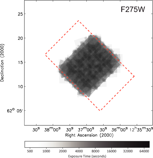
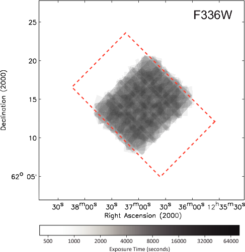
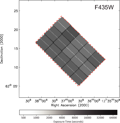
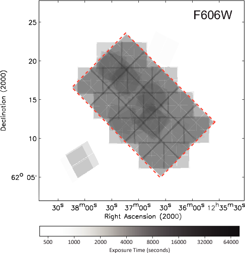
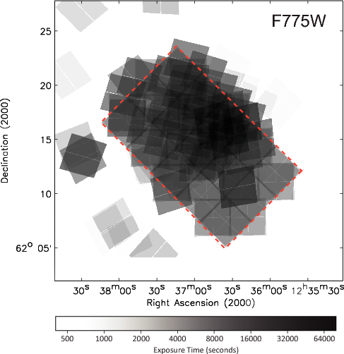
Figure 20.— Exposure maps for the bluer filters of the CANDELS GOODS-N region, including legacy ACS exposures. All exposure maps are plotted with a logarithmic stretch from 0.4 to 80 ks. The F606W will receive additional exposures that are currently shown as F814W (Fig. 21). The dotted red line indicates the fiducial GOODS ACS boundary.

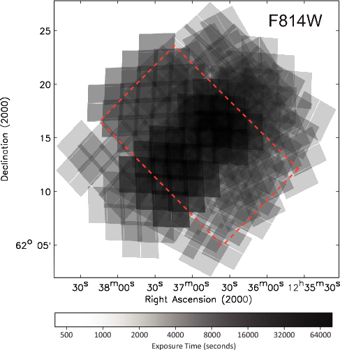
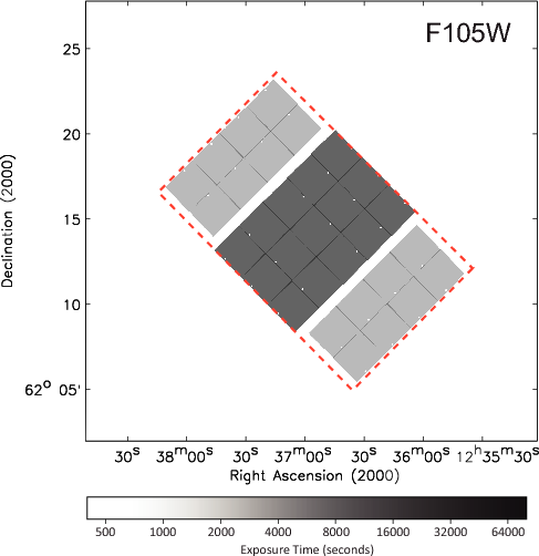
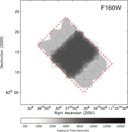
Figure 21.— Exposure maps for the redder filters of the CANDELS GOODS-N region, including legacy ACS exposures. All exposure maps are plotted with a logarithmic stretch from 0.4 to 80 ks. Virtually all of the F814W exposures shown here are from the CANDELS program. A small portion of these will instead be taken with the F606W and F850LP filters, when our GOODS-N filter assignments are finalized. The dotted red line indicates the fiducial GOODS ACS boundary.

Figures 22a,b show the curves of area versus exposure depth for each of the ACS and WFC3 filters that will comprise the CANDELS GOODS-N field. Each of these area vs. depth plots considers only the area within the footprint of CANDELS images but includes all legacy ACS imaging within that region. The curves for F606W and F850LP will be slightly augmented at the expense of F814W, once the GOODS-N filter assignments have been finalized.

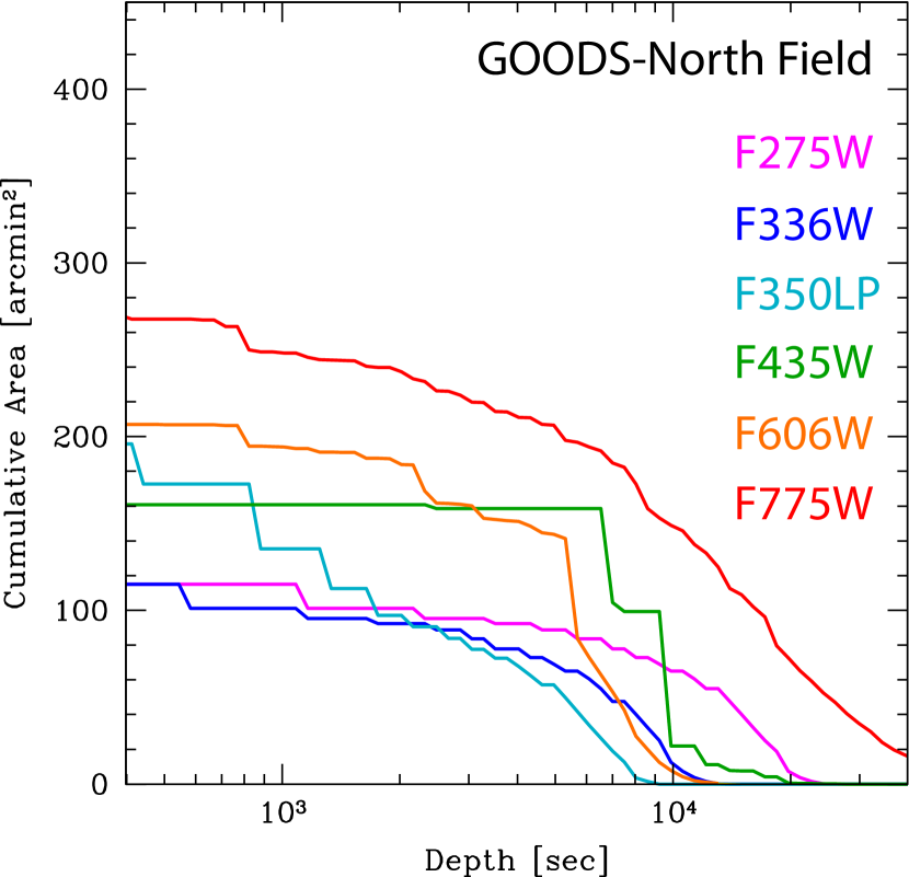
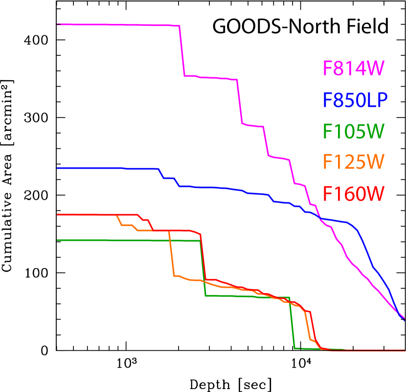
Figure 22.— Cumulative area vs. depth profiles of the CANDELS GOODS-N field, including legacy ACS exposures. The areas are limited to the footprint of the CANDELS images. The curves for F606W and F850LP will be slightly augmented at the expense of F814W, once our GOODS-N filter assignments have been finalized.

The aggregate areas, HST exposure times, and filter sensitivities of the Wide and Deep programs are summarized in Table 6. Given the heterogeneous ancillary HST data in CANDELS, the exposure depths vary substantially from field to field and within each field for both Wide and Deep programs (see Figs. 16, 19, and 22). We therefore quote an approximate lower limit to the filter sensitivities in Table 6. Point-source limiting magnitudes correspond to the “optimal” signal-to-noise estimate provided by the HST exposure time calculator. Extended-source limiting magnitudes correspond to $5\times$ the photometric error within a $0.2$ arcsec² aperture. Note that the GOODS-S ERS field is entirely legacy HST imaging except for CANDELS ACS parallels to the GOODS-S Deep.

Table 6CANDELS Areas, Exposure, and $5\sigma$ Sensitivities

HST	Exposure	Pt.-Src. $5\sigma$	Extended $5\sigma$
Filter	[s]	[mag]	[mag]
CANDELS/Deep Program
GOODS-South Field ($\sim 7\arcmin\times 10\arcmin$)
F435W	7200	28.7	27.7
F606W	10600	29.3	28.3
F775W	8600	28.5	27.6
F814W	31900	29.4	28.4
F850LP	28600	28.5	27.6
F105W	8100	28.2	28.1
F125W	9100	27.9	27.9
F160W	9200	27.6	27.6
GOODS-North Field ($\sim 7\arcmin\times 10\arcmin$)
F275W	13500	29.1	27.9
F336W	6300	28.9	27.7
F435W	7200	28.7	27.7
F606W	8000	29.1	28.2
F775W	18600	28.9	28.0
F814W	32000	29.4	28.4
F850LP	30000	28.5	27.6
F105W	8900	28.3	28.2
F125W	10600	28.0	28.0
F160W	11200	27.7	27.8
CANDELS/Wide Program
UDS Field ($\sim 9\arcmin\times 24\arcmin$)
F606W	2800	28.4	27.5
F814W	5700	28.4	27.5
F125W	1900	27.0	27.0
F160W	3300	27.1	27.1
EGS Field ($\sim 7\arcmin\times 26\arcmin$)
F606W	5700	28.9	28.0
F814W	10000	28.8	27.9
F125W	1900	27.2	27.1
F160W	3600	27.3	27.4
COSMOS Field ($\sim 9\arcmin\times 24\arcmin$)
F606W	3300	28.5	27.6
F814W	6900	28.5	27.6
F125W	1900	27.0	27.0
F160W	3200	27.1	27.1
GOODS-South Flanking ($\sim 4\arcmin\times 10\arcmin$)
F435W	7200	28.7	27.8
F606W	8600	29.2	28.2
F775W	7000	28.4	27.4
F814W	7500	28.6	27.7
F850LP	30000	28.5	27.6
F105W	2700	27.6	27.5
F125W	2100	27.1	27.1
F160W	2100	26.8	26.8
GOODS-South ERS ($\sim 4\arcmin\times 9\arcmin$)
F225W	5700	27.7	26.6
F275W	5700	27.8	26.7
F336W	2800	27.7	26.6
F435W	7200	28.7	27.8
F606W	5500	28.9	28.0
F775W	7000	28.4	27.5
F814W	10000	28.7	27.8
F850LP	17200	28.2	27.3
F098M	5000	27.5	27.4
F125W	5000	27.6	27.5
F160W	5000	27.3	27.3
GOODS-North Flanking (2 @ $\sim 4\arcmin\times 9\arcmin$)
F435W	7200	28.7	27.7
F606W	5600	28.9	28.0
F775W	8100	28.4	27.5
F814W	12000	28.8	27.9
F850LP	25000	28.4	27.5
F105W	2900	27.7	27.5
F125W	1900	27.1	27.0
F160W	2800	27.0	27.0

6.3. Scheduling of Observations

We summarize the currently planned timetable of CANDELS epochs in Figure 23, including dates of execution, orbits per epoch, HST orientation, and a five-character alphanumeric descriptor that will prefix the given epoch’s CANDELS data releases (see Koekemoer et al. 2011 for details). The entries are color-coded by field, in chronological order with GOODS-S (cyan), UDS (orange), EGS (blue), COSMOS (yellow), and GOODS-N (magenta). The very first entry is a single test orbit to verify sensitivities and dithering pattern, taken in the GOODS-S region (at the northwest corner of the ERS) and included in the Program 12061 PhaseII description. The portions of the CANDELS program that have been assigned HST Program IDs at the time of writing are listed in the last column of the timetable.

With ten SN Ia-search epochs spaced every $\sim 52$ days, each CANDELS Deep campaign must execute steadily across nearly 1.5 years. To avoid overlap of epochs among the different CANDELS fields during the three-year execution of the program, we started the GOODS-S observations early in Cycle 18 and plan to begin the GOODS-N observations almost immediately after GOODS-S completes, in the latter part of Cycle 19. The last GOODS-N epoch is planned to complete near the end of Cycle 20. The slightly longer duration of the GOODS-S program is due to the couple of months in Spring 2011 when the field is too close to the sun for HST observations, and the inter-epoch gap must be extended well beyond the 52 d optimal for SN Ia-searching. GOODS-N, on the other hand, can be observed year-round.

In the GOODS-N field, the $\sim 52$ day cadence for optimal detection of extreme-redshift SNe Ia fortuitously matches the intervals between CVZ opportunities. Our intention is to align the CANDELS GOODS-N observing schedule with the CVZ cadence in order to obtain WFC3/UVIS F275W and F336W exposures in the Deep region during the bright-earth portion of the HST orbits, at no additional cost in orbits to the program.

The CANDELS/Wide campaigns, whose tightly-constrained HST orientations must be held fixed for $>\!60$d spans, are scheduled to avoid overlap with the CANDELS/Deep epochs, and to distribute the CANDELS HST orbit allocation as evenly as possible across the full three years of the Multi-Cycle Treasury Program.

In all cases we have tried to compress the epochs into as short an interval as reasonably schedulable with HST, and to perform all observations in a given epoch at identical HST orientation. It is inevitable that the large WFC3/IR rasters include a small fraction of tiles with no suitable HST guide-stars at exactly the desired orientation. In the rare cases that the nearest guide-star orientation to our desired epoch’s value is unobservable during an epoch’s scheduled window, or when a guide-star failure occurs in the course of program execution and the pointing must be re-observed, the corresponding tile is by necessity observed outside the window listed in the timetable.

The up-to-date Phase II-level description of the CANDELS HST observations, including variances from the plans described herein because of guide-star failures, scheduling incompatibilities, etc., may be obtained by querying the corresponding Program ID status on the STScI website.

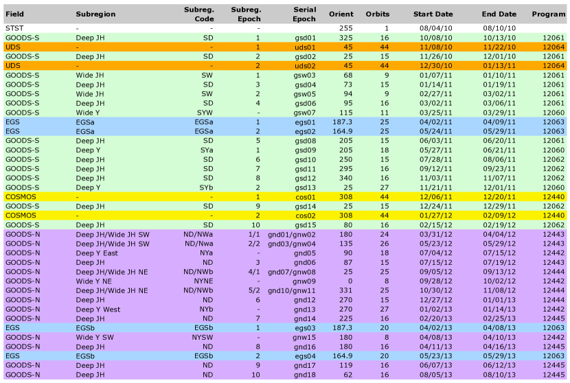
Figure 23.— Timetable of CANDELS epochs. The individual fields are color coded as follows: GOODS-S (cyan), UDS (orange), EGS (blue), COSMOS (yellow), and GOODS-N (magenta). See text for a full description of the columns.

7. Summary

We have presented an overview of the Cosmic Assembly Near-infrared Extragalactic Legacy Survey (CANDELS), an ongoing HST imaging survey of five pre-eminent extragalactic deep fields, allocated approximately ten percent of HST’s available observing time for three years. We intend this overview to serve as a reference for the anticipated wealth of science enabled by this survey, underway since Fall 2010. We have enumerated the CANDELS collaboration’s principal science goals that have guided the survey design, but we also emphasize that CANDELS is an HST Treasury survey with strong commitment to rapid dissemination of data products for use by the wider astronomical community. Our science goals may be roughly segregated into the topics of “Cosmic Dawn” ($z\gtrsim 6$), “Cosmic High Noon” ($z\approx 2$), SN cosmology, and moderate-$z$ galaxies’ far-UV. We refer the reader to Table 2 for an outline of these science goals.

We have described the specifics of our observing strategy for achieving the aforementioned science goals, in as complete detail as possible for a survey still in its early stages and not yet fully evolved from conception to implementation. We have presented justifications for the five chosen CANDELS fields, with attention to the ancillary data that are a crucial complement to achieve our goals. We have also provided our best estimate of the CANDELS HST schedule of observations, aggregate exposure maps, and limiting sensitivities. These sensitivity estimates, while useful benchmarks for our survey design, will undoubtedly vary somewhat from the delivered mosaics’ sensitivities, which we will duly report in our forthcoming papers on CANDELS data releases.

The HST images we have received to date have been completely processed through the CANDELS pipeline, described in the companion paper by Koekemoer et al. (2011). There we present the details of the calibration procedures and image processing, as well as the resulting public-release mosaic data products for each field. In brief, we create a set of single-epoch combined mosaics in all the filters that are obtained in each epoch separately, as well as a set of combined mosaics that include all the data so far obtained on a given field. We perform a series of specialized calibration steps that include improved treatment of detector warm pixels and persistence in the WFC3/IR images, and correction for bias striping, amplifier crosstalk, and CTE degradation in the ACS images. Full details may be found in Koekemoer et al. (2011), as well as the public CANDELS website. Three months after the observations of each CANDELS epoch are completed (see Fig. 23), we release the calibrated mosaic images to the public via the STScI archive. At the time of writing, we have already released the first several GOODS-S epochs, the full UDS campaign, and the first EGS campaign (covering over half that field). We strongly encourage the astronomical community to make use of CANDELS to advance their own research.

8. Acknowledgments

We would like to thank our Program Coordinators, Tricia Royle and Beth Perriello, along with the rest of the Hubble planning team, for their efforts to schedule this challenging program. The WFC3 team has made substantial contributions to the program by calibrating and characterizing the instrument, and have provided much useful advice. Rychard Bouwens gave helpful input on the observing strategy for the CANDELS/Deep survey. John Mackenty suggested using $2\times 2$ on-chip binning for the UV observations, which significantly improves the signal-to-noise ratio of those observations. The CANDELS observations would not have been possible without the contributions of hundreds of other individuals to the Hubble missions and the development and installation of new instruments.

Support for HST Programs GO-12060 and GO-12099 was provided by NASA through grants from the Space Telescope Science Institute, which is operated by the Association of Universities for Research in Astronomy, Inc., under NASA contract NAS5-26555. A. Fontana acknowledges support from agreement ASI-INAF I/009/10/0.

Facilities: HST (WFC3)

References

- Abraham et al. (1996) Abraham, R. G., Tanvir, N. R., Santiago, B. X., Ellis, R. S., Glazebrook, K., & van den Bergh, S. 1996, MNRAS, 279, L47
- Aguirre & Bolocam Galactic Plane Collaboration (2007) Aguirre, J. E., & Bolocam Galactic Plane Collaboration. 2007, in Bulletin of the American Astronomical Society, Vol. 38, American Astronomical Society Meeting Abstracts, 882
- Aird et al. (2008) Aird, J., Nandra, K., Georgakakis, A., Laird, E. S., Steidel, C. C., & Sharon, C. 2008, MNRAS, 387, 883
- Alexander et al. (2003) Alexander, D. M., et al. 2003, AJ, 126, 539
- Alexander et al. (2008) Alexander, D. M., et al. 2008, AJ, 135, 1968
- Alonso-Herrero et al. (2006) Alonso-Herrero, A., et al. 2006, ApJ, 640, 167
- Babul & Rees (1992) Babul, A., & Rees, M. J. 1992, MNRAS, 255, 346
- Balestra et al. (2010) Balestra, I., et al. 2010, A&A, 512, A12
- Barger et al. (2008) Barger, A. J., Cowie, L. L., & Wang, W.-H. 2008, ApJ, 689, 687
- Becker & Iben (1980) Becker, S. A., & Iben, I., Jr. 1980, ApJ, 237, 111
- Beckwith et al. (2006) Beckwith, S. V. W., et al. 2006, AJ, 132, 1729
- Behroozi et al. (2010) Behroozi, P. S., Conroy, C., & Wechsler, R. H. 2010, ApJ, 717, 379
- Bell et al. (2004) Bell, E. F., et al. 2004, ApJ, 608, 752
- Botticella et al. (2008) Botticella, M. T., et al. 2008, A&A, 479, 49
- Bournaud et al. (2007) Bournaud, F., Elmegreen, B. G., & Elmegreen, D. M. 2007, ApJ, 670, 237
- Bouwens et al. (2007) Bouwens, R. J., Illingworth, G. D., Franx, M., & Ford, H. 2007, ApJ, 670, 928
- Bouwens et al. (2008) Bouwens, R. J., Illingworth, G. D., Franx, M., & Ford, H. 2008, ApJ, 686, 230
- Bouwens et al. (2010a) Bouwens, R. J., et al. 2010a, ApJ, 709, L133
- Bouwens et al. (2010b) Bouwens, R. J., et al. 2010b, ApJ, 708, L69
- Bouwens et al. (2011a) Bouwens, R. J., et al. 2011a, Nature, 469, 504
- Bouwens et al. (2011b) Bouwens, R. J., et al. 2011b, ApJ, 737, 90
- Brinchmann et al. (2004) Brinchmann, J., Charlot, S., White, S. D. M., Tremonti, C., Kauffmann, G., Heckman, T., & Brinkmann, J. 2004, MNRAS, 351, 1151
- Brown et al. (2007) Brown, M. J. I., Dey, A., Jannuzi, B. T., Brand, K., Benson, A. J., Brodwin, M., Croton, D. J., & Eisenhardt, P. R. 2007, ApJ, 654, 858
- Brusa et al. (2009) Brusa, M., et al. 2009, ApJ, 693, 8
- Bullock et al. (2000) Bullock, J. S., Kravtsov, A. V., & Weinberg, D. H. 2000, ApJ, 539, 517
- Capak et al. (2004) Capak, P., et al. 2004, AJ, 127, 180
- Cardamone et al. (2010) Cardamone, C. N., et al. 2010, ApJS, 189, 270
- Castellano et al. (2010a) Castellano, M., et al. 2010a, A&A, 511, A20
- Castellano et al. (2010b) Castellano, M., et al. 2010b, A&A, 524, A28
- Ceverino et al. (2010) Ceverino, D., Dekel, A., & Bournaud, F. 2010, MNRAS, 404, 2151
- Chary et al. (2008) Chary, R.-R., Cooray, A., & Sullivan, I. 2008, ApJ, 681, 53
- Chary et al. (2007) Chary, R.-R., Teplitz, H. I., Dickinson, M. E., Koo, D. C., Le Floc’h, E., Marcillac, D., Papovich, C., & Stern, D. 2007, ApJ, 665, 257
- Cimatti et al. (2008) Cimatti, A., et al. 2008, A&A, 482, 21
- Cirasuolo et al. (2007) Cirasuolo, M., et al. 2007, MNRAS, 380, 585
- Clarke & Oey (2002) Clarke, C., & Oey, M. S. 2002, MNRAS, 337, 1299
- Coil et al. (2004) Coil, A. L., et al. 2004, ApJ, 609, 525
- Conroy et al. (2006) Conroy, C., Wechsler, R. H., & Kravtsov, A. V. 2006, ApJ, 647, 201
- Conselice (2006) Conselice, C. J. 2006, ApJ, 638, 686
- Conselice et al. (2003) Conselice, C. J., Bershady, M. A., Dickinson, M., & Papovich, C. 2003, AJ, 126, 1183
- Conselice et al. (2011a) Conselice, C. J., et al. 2011, MNRAS, 413, 80
- Conselice et al. (2011b) Conselice, C. J., et al. 2011, ArXiv e-prints (1105.2522)
- Cooper et al. (2011) Cooper, M. C., et al. 2011, ApJS, 193, 14
- Cooray et al. (2004) Cooray, A., Bock, J. J., Keatin, B., Lange, A. E., & Matsumoto, T. 2004, ApJ, 606, 611
- Coppin et al. (2008) Coppin, K. E. K., et al. 2008, MNRAS, 389, 45
- Covington et al. (2011) Covington, M. D., Primack, J. R., Porter, L. A., Croton, D. J., Somerville, R. S., & Dekel, A. 2011, MNRAS, 415, 3135
- Croton et al. (2006) Croton, D. J., et al. 2006, MNRAS, 365, 11
- Cuillandre et al. (2001) Cuillandre, J.-C., Starr, B., Isani, S., McDonald, J. S., & Luppino, G. 2001, in Astronomical Society of the Pacific Conference Series, Vol. 232, The New Era of Wide Field Astronomy, ed. R. Clowes, A. Adamson, & G. Bromage, 398
- Daddi et al. (2007a) Daddi, E., et al. 2007a, ApJ, 670, 173
- Daddi et al. (2007b) Daddi, E., et al. 2007b, ApJ, 670, 156
- Daddi et al. (2010) Daddi, E., et al. 2010, ApJ, 714, L118
- Daddi et al. (2005) Daddi, E., et al. 2005, ApJ, 626, 680
- Dahlen et al. (2008) Dahlen, T., Strolger, L.-G., & Riess, A. G. 2008, ApJ, 681, 462
- Dahlen et al. (2004) Dahlen, T., et al. 2004, ApJ, 613, 189
- Davis et al. (2003) Davis, M., et al. 2003, in Presented at the Society of Photo-Optical Instrumentation Engineers (SPIE) Conference, Vol. 4834, Society of Photo-Optical Instrumentation Engineers (SPIE) Conference Series, ed. P. Guhathakurta, 161
- Davis et al. (2007) Davis, M., et al. 2007, ApJ, 660, L1
- Dekel & Birnboim (2006) Dekel, A., & Birnboim, Y. 2006, MNRAS, 368, 2
- Dekel et al. (2009) Dekel, A., et al. 2009, Nature, 457, 451
- Di Matteo et al. (2005) Di Matteo, T., Springel, V., & Hernquist, L. 2005, Nature, 433, 604
- Dickinson et al. (2003) Dickinson, M., Giavalisco, M., & GOODS Team. 2003, in The Mass of Galaxies at Low and High Redshift, ed. R. Bender & A. Renzini, 324
- Dickinson et al. (2004) Dickinson, M., et al. 2004, ApJ, 600, L99
- Dilday et al. (2010) Dilday, B., et al. 2010, ApJ, 713, 1026
- Domínguez et al. (2001) Domínguez, I., Höflich, P., & Straniero, O. 2001, ApJ, 557, 279
- Donley et al. (2010) Donley, J. L., Rieke, G. H., Alexander, D. M., Egami, E., & Pérez-González, P. G. 2010, ApJ, 719, 1393
- Donley et al. (2008) Donley, J. L., Rieke, G. H., Pérez-González, P. G., & Barro, G. 2008, ApJ, 687, 111
- Driver et al. (1995) Driver, S. P., Windhorst, R. A., & Griffiths, R. E. 1995, ApJ, 453, 48
- Dunlop et al. (2007) Dunlop, J. S., Cirasuolo, M., & McLure, R. J. 2007, MNRAS, 376, 1054
- Dutton et al. (2011) Dutton, A. A., et al. 2011, MNRAS, 410, 1660
- Dutton & van den Bosch (2009) Dutton, A. A., & van den Bosch, F. C. 2009, MNRAS, 396, 141
- Ebrero et al. (2009) Ebrero, J., et al. 2009, A&A, 493, 55
- Elmegreen et al. (2008) Elmegreen, B. G., Bournaud, F., & Elmegreen, D. M. 2008, ApJ, 688, 67
- Elmegreen et al. (2009) Elmegreen, B. G., Elmegreen, D. M., Fernandez, M. X., & Lemonias, J. J. 2009, ApJ, 692, 12
- Eyles et al. (2007) Eyles, L. P., Bunker, A. J., Ellis, R. S., Lacy, M., Stanway, E. R., Stark, D. P., & Chiu, K. 2007, MNRAS, 374, 910
- Eyles et al. (2005) Eyles, L. P., Bunker, A. J., Stanway, E. R., Lacy, M., Ellis, R. S., & Doherty, M. 2005, MNRAS, 364, 443
- Faber et al. (2003) Faber, S. M., et al. 2003, in Presented at the Society of Photo-Optical Instrumentation Engineers (SPIE) Conference, Vol. 4841, Society of Photo-Optical Instrumentation Engineers (SPIE) Conference Series, ed. M. Iye & A. F. M. Moorwood, 1657
- Faber et al. (2007) Faber, S. M., et al. 2007, ApJ, 665, 265
- Fan et al. (2006) Fan, X., Carilli, C. L., & Keating, B. 2006, ARA&A, 44, 415
- Fan et al. (2003) Fan, X., et al. 2003, AJ, 125, 1649
- Fernandez et al. (2010) Fernandez, E. R., Komatsu, E., Iliev, I. T., & Shapiro, P. R. 2010, ApJ, 710, 1089
- Ferrarese & Merritt (2000) Ferrarese, L., & Merritt, D. 2000, ApJ, 539, L9
- Finkelstein et al. (2011) Finkelstein, S. L., Cohen, S. H., Moustakas, J., Malhotra, S., Rhoads, J. E., & Papovich, C. 2011, ApJ, 735, 5
- Finlator et al. (2011) Finlator, K., Oppenheimer, B. D., & Davé, R. 2011, MNRAS, 410, 1703
- Fontana et al. (2010) Fontana, A., et al. 2010, ApJ, 725, L205
- Förster Schreiber et al. (2009) Förster Schreiber, N. M., et al. 2009, ApJ, 706, 1364
- Franx et al. (2008) Franx, M., van Dokkum, P. G., Schreiber, N. M. F., Wuyts, S., Labbé, I., & Toft, S. 2008, ApJ, 688, 770
- Fujita et al. (2002) Fujita, Y., Sarazin, C. L., Nagashima, M., & Yano, T. 2002, ApJ, 577, 11
- Gallego et al. (1997) Gallego, J., Zamorano, J., Rego, M., & Vitores, A. G. 1997, ApJ, 475, 502
- Gebhardt et al. (2000) Gebhardt, K., et al. 2000, ApJ, 539, L13
- Giacconi et al. (2002) Giacconi, R., et al. 2002, ApJS, 139, 369
- Giavalisco et al. (2004) Giavalisco, M., et al. 2004, ApJ, 600, L93
- Giavalisco et al. (1996) Giavalisco, M., Steidel, C. C., & Macchetto, F. D. 1996, ApJ, 470, 189
- Gnedin et al. (2008) Gnedin, N. Y., Kravtsov, A. V., & Chen, H.-W. 2008, ApJ, 672, 765
- González et al. (2010) González, V., Labbé, I., Bouwens, R. J., Illingworth, G., Franx, M., Kriek, M., & Brammer, G. B. 2010, ApJ, 713, 115
- Grazian et al. (2011) Grazian, A., et al. 2011, A&A, 532, A33
- Greggio et al. (2008) Greggio, L., Renzini, A., & Daddi, E. 2008, MNRAS, 388, 829
- Grogin et al. (2005) Grogin, N. A., et al. 2005, ApJ, 627, L97
- Gwyn (2008) Gwyn, S. D. J. 2008, PASP, 120, 212
- Häring & Rix (2004) Häring, N., & Rix, H.-W. 2004, ApJ, 604, L89
- Hasinger et al. (2007) Hasinger, G., et al. 2007, ApJS, 172, 29
- Hopkins & Beacom (2006) Hopkins, A. M., & Beacom, J. F. 2006, ApJ, 651, 142
- Hopkins et al. (2006) Hopkins, P. F., Hernquist, L., Cox, T. J., Di Matteo, T., Robertson, B., & Springel, V. 2006, ApJS, 163, 1
- Hopkins et al. (2008) Hopkins, P. F., Hernquist, L., Cox, T. J., & Kereš, D. 2008, ApJS, 175, 356
- Immeli et al. (2004) Immeli, A., Samland, M., Westera, P., & Gerhard, O. 2004, ApJ, 611, 20
- Ivison et al. (2007) Ivison, R. J., et al. 2007, ApJ, 660, L77
- Iwata et al. (2009) Iwata, I., et al. 2009, ApJ, 692, 1287
- Jonsson et al. (2010) Jonsson, P., Groves, B. A., & Cox, T. J. 2010, MNRAS, 403, 17
- Juneau et al. (2005) Juneau, S., et al. 2005, ApJ, 619, L135
- Kashlinsky et al. (2005) Kashlinsky, A., Arendt, R. G., Mather, J., & Moseley, S. H. 2005, Nature, 438, 45
- Kauffmann et al. (2003) Kauffmann, G., et al. 2003, MNRAS, 341, 33
- Kellermann et al. (2008) Kellermann, K. I., Fomalont, E. B., Mainieri, V., Padovani, P., Rosati, P., Shaver, P., Tozzi, P., & Miller, N. 2008, ApJS, 179, 71
- Kereš et al. (2005) Kereš, D., Katz, N., Weinberg, D. H., & Davé, R. 2005, MNRAS, 363, 2
- Klypin et al. (2010) Klypin, A., Trujillo-Gomez, S., & Primack, J. 2010, ArXiv e-prints (1002.3660)
- Kobayashi & Nomoto (2009) Kobayashi, C., & Nomoto, K. 2009, ApJ, 707, 1466
- Koekemoer et al. (2004) Koekemoer, A. M., et al. 2004, ApJ, 600, L123
- Koekemoer et al. (2007) Koekemoer, A. M., et al. 2007, ApJS, 172, 196
- Koekemoer et al. (2011) Koekemoer, A. M., et al. 2011, ApJS, submitted
- Kuznetsova et al. (2008) Kuznetsova, N., et al. 2008, ApJ, 673, 981
- Labbé et al. (2010) Labbé, I., et al. 2010, ApJ, 716, L103
- Laird et al. (2009) Laird, E. S., et al. 2009, ApJS, 180, 102
- Law et al. (2011) Law, D. R., et al. 2011, ArXiv e-prints (1107.3137)
- Lawrence et al. (2007) Lawrence, A., et al. 2007, MNRAS, 379, 1599
- Le Fèvre et al. (2004) Le Fèvre, O., et al. 2004, A&A, 428, 1043
- Lee et al. (2009) Lee, K.-S., Giavalisco, M., Conroy, C., Wechsler, R. H., Ferguson, H. C., Somerville, R. S., Dickinson, M. E., & Urry, C. M. 2009, ApJ, 695, 368
- Lee et al. (2006) Lee, K.-S., Giavalisco, M., Gnedin, O. Y., Somerville, R. S., Ferguson, H. C., Dickinson, M., & Ouchi, M. 2006, ApJ, 642, 63
- Lehnert et al. (2010) Lehnert, M. D., et al. 2010, Nature, 467, 940
- Li et al. (2007) Li, Y., et al. 2007, ApJ, 665, 187
- Lilly et al. (1996) Lilly, S. J., Le Fevre, O., Hammer, F., & Crampton, D. 1996, ApJ, 460, L1
- Lilly et al. (2007) Lilly, S. J., et al. 2007, ApJS, 172, 70
- Lotz et al. (2008) Lotz, J. M., Jonsson, P., Cox, T. J., & Primack, J. R. 2008, MNRAS, 391, 1137
- Lotz et al. (2004) Lotz, J. M., Primack, J., & Madau, P. 2004, AJ, 128, 163
- Lu et al. (2010) Lu, Y., Mo, H. J., Weinberg, M. D., & Katz, N. S. 2010, ArXiv e-prints (1004.2518)
- Madau et al. (1996) Madau, P., Ferguson, H. C., Dickinson, M. E., Giavalisco, M., Steidel, C. C., & Fruchter, A. 1996, MNRAS, 283, 1388
- Magorrian et al. (1998) Magorrian, J., et al. 1998, AJ, 115, 2285
- Mannucci et al. (2005) Mannucci, F., Della Valle, M., Panagia, N., Cappellaro, E., Cresci, G., Maiolino, R., Petrosian, A., & Turatto, M. 2005, A&A, 433, 807
- Marchesini et al. (2009) Marchesini, D., van Dokkum, P. G., Förster Schreiber, N. M., Franx, M., Labbé, I., & Wuyts, S. 2009, ApJ, 701, 1765
- Marulli et al. (2008) Marulli, F., Bonoli, S., Branchini, E., Moscardini, L., & Springel, V. 2008, MNRAS, 385, 1846
- McLure et al. (2010) McLure, R. J., Dunlop, J. S., Cirasuolo, M., Koekemoer, A. M., Sabbi, E., Stark, D. P., Targett, T. A., & Ellis, R. S. 2010, MNRAS, 403, 960
- McLure et al. (2011) McLure, R. J., et al. 2011, ArXiv e-prints (1102.4881)
- Mignoli et al. (2005) Mignoli, M., et al. 2005, A&A, 437, 883
- Mobasher et al. (2005) Mobasher, B., et al. 2005, ApJ, 635, 832
- Morrison et al. (2010) Morrison, G. E., Owen, F. N., Dickinson, M., Ivison, R. J., & Ibar, E. 2010, ApJS, 188, 178
- Naab et al. (2009) Naab, T., Johansson, P. H., & Ostriker, J. P. 2009, ApJ, 699, L178
- Newman & Davis (2002) Newman, J. A., & Davis, M. 2002, ApJ, 564, 567
- Noeske et al. (2007) Noeske, K. G., et al. 2007, ApJ, 660, L43
- Noguchi (1999) Noguchi, M. 1999, ApJ, 514, 77
- Nonino et al. (2009) Nonino, M., et al. 2009, ApJS, 183, 244
- Oesch et al. (2010) Oesch, P. A., et al. 2010, ApJ, 725, L150
- Oesch et al. (2011) Oesch, P. A., et al. 2011, ArXiv e-prints (1105.2297)
- Oke & Gunn (1983) Oke, J. B., & Gunn, J. E. 1983, ApJ, 266, 713
- Ota et al. (2010) Ota, K., et al. 2010, ApJ, 722, 803
- Ouchi et al. (2009) Ouchi, M., et al. 2009, ApJ, 706, 1136
- Ouchi et al. (2010) Ouchi, M., et al. 2010, ApJ, 723, 869
- Page et al. (2007) Page, L., et al. 2007, ApJS, 170, 335
- Panagia et al. (2007) Panagia, N., Della Valle, M., & Mannucci, F. 2007, in American Institute of Physics Conference Series, Vol. 924, The Multicolored Landscape of Compact Objects and Their Explosive Origins, ed. T. di Salvo, G. L. Israel, L. Piersant, L. Burderi, G. Matt, A. Tornambe, & M. T. Menna, 373
- Papovich et al. (2011) Papovich, C., Finkelstein, S. L., Ferguson, H. C., Lotz, J. M., & Giavalisco, M. 2011, MNRAS, 412, 1123
- Papovich et al. (2006) Papovich, C., et al. 2006, ApJ, 640, 92
- Pérez-González et al. (2008) Pérez-González, P. G., et al. 2008, ApJ, 675, 234
- Perlmutter et al. (1999) Perlmutter, S., et al. 1999, ApJ, 517, 565
- Pierce et al. (2007) Pierce, C. M., et al. 2007, ApJ, 660, L19
- Pope et al. (2008) Pope, A., et al. 2008, ApJ, 675, 1171
- Popesso et al. (2009) Popesso, P., et al. 2009, A&A, 494, 443
- Ravikumar et al. (2007) Ravikumar, C. D., et al. 2007, A&A, 465, 1099
- Ravindranath et al. (2006) Ravindranath, S., et al. 2006, ApJ, 652, 963
- Reddy et al. (2006) Reddy, N. A., Steidel, C. C., Erb, D. K., Shapley, A. E., & Pettini, M. 2006, ApJ, 653, 1004
- Reddy et al. (2008) Reddy, N. A., Steidel, C. C., Pettini, M., Adelberger, K. L., Shapley, A. E., Erb, D. K., & Dickinson, M. 2008, ApJS, 175, 48
- Retzlaff et al. (2010) Retzlaff, J., Rosati, P., Dickinson, M., Vandame, B., Rité, C., Nonino, M., Cesarsky, C., & GOODS Team. 2010, A&A, 511, A50
- Rhodes et al. (2000) Rhodes, J., Refregier, A., & Groth, E. J. 2000, ApJ, 536, 79
- Rhook & Haehnelt (2008) Rhook, K. J., & Haehnelt, M. G. 2008, MNRAS, 389, 270
- Riess et al. (1998) Riess, A. G., et al. 1998, AJ, 116, 1009
- Riess et al. (2004) Riess, A. G., et al. 2004, ApJ, 607, 665
- Riess & Livio (2006) Riess, A. G., & Livio, M. 2006, ApJ, 648, 884
- Riess et al. (2007) Riess, A. G., et al. 2007, ApJ, 659, 98
- Ruiz-Lapuente & Canal (2000) Ruiz-Lapuente, P., & Canal, R. 2000, ArXiv Astrophysics e-prints (astro-ph/0009312)
- Ryan-Weber et al. (2006) Ryan-Weber, E. V., Pettini, M., & Madau, P. 2006, MNRAS, 371, L78
- Sanders et al. (2007) Sanders, D. B., et al. 2007, ApJS, 172, 86
- Sanders et al. (1988) Sanders, D. B., Soifer, B. T., Elias, J. H., Madore, B. F., Matthews, K., Neugebauer, G., & Scoville, N. Z. 1988, ApJ, 325, 74
- Scannapieco & Bildsten (2005) Scannapieco, E., & Bildsten, L. 2005, ApJ, 629, L85
- Schechter (1976) Schechter, P. 1976, ApJ, 203, 297
- Schinnerer et al. (2004) Schinnerer, E., et al. 2004, AJ, 128, 1974
- Schinnerer et al. (2007) Schinnerer, E., et al. 2007, ApJS, 172, 46
- Scoville et al. (2007) Scoville, N., et al. 2007, ApJS, 172, 1
- Sekiguchi et al. (2004) Sekiguchi, K., et al. 2004, Subaru/XMM-Newton Deep Survey, ed. Tanikawa, K., Imanishi, M., Miyoshi, M., Muramatsu, T., Sekii, T., Sôma, M., Ueda, A., Yamashita, Y., & Yasuda, N. 40
- Shapley et al. (2003) Shapley, A. E., Steidel, C. C., Pettini, M., & Adelberger, K. L. 2003, ApJ, 588, 65
- Shapley et al. (2006) Shapley, A. E., Steidel, C. C., Pettini, M., Adelberger, K. L., & Erb, D. K. 2006, ApJ, 651, 688
- Shim et al. (2009) Shim, H., Colbert, J., Teplitz, H., Henry, A., Malkan, M., McCarthy, P., & Yan, L. 2009, ApJ, 696, 785
- Siana et al. (2010) Siana, B., et al. 2010, ApJ, 723, 241
- Silverman et al. (2010) Silverman, J. D., et al. 2010, ApJS, 191, 124
- Simpson et al. (2006) Simpson, C., et al. 2006, MNRAS, 372, 741
- Somerville et al. (2008a) Somerville, R. S., et al. 2008a, ApJ, 672, 776
- Somerville et al. (2008b) Somerville, R. S., Hopkins, P. F., Cox, T. J., Robertson, B. E., & Hernquist, L. 2008b, MNRAS, 391, 481
- Songaila (2001) Songaila, A. 2001, ApJ, 561, L153
- Spergel et al. (2007) Spergel, D. N., et al. 2007, ApJS, 170, 377
- Steidel et al. (2003) Steidel, C. C., Adelberger, K. L., Shapley, A. E., Pettini, M., Dickinson, M., & Giavalisco, M. 2003, ApJ, 592, 728
- Strolger et al. (2010) Strolger, L.-G., Dahlen, T., & Riess, A. G. 2010, ApJ, 713, 32
- Strolger et al. (2005) Strolger, L.-G., Riess, A. G., & Dahlen, T. 2005, in Astronomical Society of the Pacific Conference Series, Vol. 342, 1604-2004: Supernovae as Cosmological Lighthouses, ed. M. Turatto, S. Benetti, L. Zampieri, & W. Shea, 471
- Strolger et al. (2004) Strolger, L.-G., et al. 2004, ApJ, 613, 200
- Szokoly et al. (2004) Szokoly, G. P., et al. 2004, ApJS, 155, 271
- Tacconi et al. (2010) Tacconi, L. J., et al. 2010, Nature, 463, 781
- Thompson et al. (2007a) Thompson, R. I., Eisenstein, D., Fan, X., Rieke, M., & Kennicutt, R. C. 2007a, ApJ, 657, 669
- Thompson et al. (2007b) Thompson, R. I., Eisenstein, D., Fan, X., Rieke, M., & Kennicutt, R. C. 2007b, ApJ, 666, 658
- Trac & Cen (2007) Trac, H., & Cen, R. 2007, ApJ, 671, 1
- Trenti et al. (2011) Trenti, M., et al. 2011, ApJ, 727, L39
- Treu et al. (2005) Treu, T., Ellis, R. S., Liao, T. X., & van Dokkum, P. G. 2005, ApJ, 622, L5
- Trujillo et al. (2007) Trujillo, I., Conselice, C. J., Bundy, K., Cooper, M. C., Eisenhardt, P., & Ellis, R. S. 2007, MNRAS, 382, 109
- van den Bosch et al. (2007) van den Bosch, F. C., et al. 2007, MNRAS, 376, 841
- van Dokkum & Brammer (2010) van Dokkum, P. G., & Brammer, G. 2010, ApJ, 718, L73
- van Dokkum et al. (2008) van Dokkum, P. G., et al. 2008, ApJ, 677, L5
- van Dokkum et al. (2009) van Dokkum, P. G., et al. 2009, PASP, 121, 2
- van Dokkum et al. (2010) van Dokkum, P. G., et al. 2010, ApJ, 709, 1018
- Vanzella et al. (2005) Vanzella, E., et al. 2005, A&A, 434, 53
- Vanzella et al. (2011) Vanzella, E., et al. 2011, ApJ, 730, L35
- Weiß et al. (2009) Weiß, A., et al. 2009, ApJ, 707, 1201
- Wiklind et al. (2008) Wiklind, T., Dickinson, M., Ferguson, H. C., Giavalisco, M., Mobasher, B., Grogin, N. A., & Panagia, N. 2008, ApJ, 676, 781
- Wilkins et al. (2008) Wilkins, S. M., Trentham, N., & Hopkins, A. M. 2008, MNRAS, 385, 687
- Williams et al. (1996) Williams, R. E., et al. 1996, AJ, 112, 1335
- Willner et al. (2006) Willner, S. P., et al. 2006, AJ, 132, 2159
- Windhorst et al. (2011) Windhorst, R. A., et al. 2011, ApJS, 193, 27
- Wirth et al. (2004) Wirth, G. D., et al. 2004, AJ, 127, 3121
- Wuyts et al. (2008) Wuyts, S., Labbé, I., Schreiber, N. M. F., Franx, M., Rudnick, G., Brammer, G. B., & van Dokkum, P. G. 2008, ApJ, 682, 985
- Yan et al. (2006) Yan, H., Dickinson, M., Giavalisco, M., Stern, D., Eisenhardt, P. R. M., & Ferguson, H. C. 2006, ApJ, 651, 24
- Yan et al. (2005) Yan, H., et al. 2005, ApJ, 634, 109
- Yan et al. (2011) Yan, H., et al. 2011, ApJ, 728, L22
- Yan et al. (2010) Yan, H.-J., Windhorst, R. A., Hathi, N. P., Cohen, S. H., Ryan, R. E., O’Connell, R. W., & McCarthy, P. J. 2010, Research in Astronomy and Astrophysics, 10, 867
- Yoshikawa et al. (2010) Yoshikawa, T., et al. 2010, ApJ, 718, 112
- Zamojski et al. (2007) Zamojski, M. A., et al. 2007, ApJS, 172, 468