Observational Properties of the Metal-Poor Thick Disk of the Milky Way Galaxy and Insights into Its Origins.

Abstract

We have undertaken the study of the elemental abundances and kinematic properties of a metal-poor sample of candidate thick-disk stars selected from the RAVE spectroscopic survey of bright stars to differentiate among the present scenarios of the formation of the thick disk. In this paper, we report on a sample of 214 red giant branch, 31 red clump/horizontal branch, and 74 main-sequence/sub-giant branch metal-poor stars, which serves to augment our previous sample of only giant stars. We find that the thick disk $\rm[\alpha/Fe]$ ratios are enhanced, and have little variation ($<0.1$ dex), in agreement with our previous study. The augmented sample further allows, for the first time, investigation of the gradients in the metal-poor thick disk. For stars with $\rm[Fe/H]<-1.2$, the thick disk shows very small gradients, $<0.03\pm 0.02~{}{\rm dex~{}kpc^{-1}}$, in $\alpha$-enhancement, while we find a $+0.01\pm 0.04~{}{\rm dex~{}kpc^{-1}}$ radial gradient and a $-0.09\pm 0.05~{}{\rm dex~{}kpc^{-1}}$ vertical gradient in iron abundance. In addition, we show that the peak of the distribution of orbital eccentricities for our sample agrees better with models in which the stars that comprise the thick disk were formed primarily in the Galaxy, with direct accretion of stars contributing little. Our results thus disfavor direct accretion of stars from dwarf galaxies into the thick disk as a major contributor to the thick disk population, but cannot discriminate between alternative models for the thick disk, such as those that invoke high-redshift (gas-rich) mergers, heating of a pre-existing thin stellar disk by a minor merger, or efficient radial migration of stars.

1. Introduction

Since its identification (Gilmore & Reid, 1983), the thick disk has been shown to have distinct kinematics (e.g. Chiba & Beers, 2000; Gilmore et al., 2002; Soubiran et al., 2003) and a distinct metallicity distribution (e.g. Majewski, 1993; Chiba & Beers, 2000) from the stellar halo and thin disk of the Milky Way Galaxy. The formation history of the thick disk can provide constraints on the origins and formation of the thin disk and halo, and ultimately the Milky Way Galaxy itself. The formation mechanism of the thick disk, however, has been the subject of much discussion for decades.

Soon after the discovery of the thick disk, Jones & Wyse (1983) proposed that early star formation in a thin disk, which formed before the Galactic potential reached virial equilibrium, could be subsequently flattened by violent relaxation to form the thick disk. Later, Burkert et al. (1992) showed that a thick disk could be formed as the result of a rapid, dissipational collapse accompanied by star formation.

The first model to gain traction, however, was that in which a pre-existing thin stellar disk is heated by a merger with a fairly robust and massive satellite, around $\sim 20\%$ the mass of the disk (e.g., Quinn et al., 1993; Velazquez & White, 1999). The thick disk is then formed primarily from the stars in the ‘thickened’ disk, while some stars are directly accreted from the satellite galaxy. More recently, this model was extended to include cosmologically motivated heating by accretion and merging from many satellites (Hayashi & Chiba, 2006; Kazantzidis et al., 2008; Villalobos & Helmi, 2008), however, the most massive satellites still dominate the heating.

Another model has the thick disk forming from the direct accretion of stars from satellite galaxies (Abadi et al., 2003). Alternatively, the thick disk could have formed during a period of rapid star formation associated with multiple minor, gas-rich mergers (Brook et al., 2004, 2005). In this model, the majority of the thick disk stars are formed from the accreted gas in the primordial disk, with a small minority being directly accreted during the mergers.

Models that have more recently gained traction are those that do not necessarily require a merger history to the formation of the thick disk. Instead, the thick disk could have formed from stars that have radially migrated outward from the inner disk by resonant scattering by transient spiral arms (Sellwood & Binney, 2002; Schönrich & Binney, 2009a, b). Another model, proposed by Bournaud et al. (2009), has the thick disk forming from internal gas clumps in the disk at high redshift.

What is the best way to distinguish these models? The distributions of kinematics and metallicity provide some discriminants, and these differ between the models most strongly at the metal-poor end. While there is clearly not a simple one-to-one relationship between age and metallicity, the most metal-poor stars in general formed early, in every scenario.

Elemental abundance patterns reveal even more detailed information about the star formation history and chemical evolution of a stellar population. The ratio of $\alpha$-elemental (e.g., Mg, Si, Ca, and Ti) abundances to iron abundance is sensitive to the relative numbers of core-collapse Type II supernovae (SNe II) and Type Ia supernovae (SNe Ia) that have occurred in the past. The $\alpha$-elements are primarily synthesized in massive stars and ejected in SNe II on short timescales ($\sim 10^{7}$ yr) after the formation of the progenitor star, with the ratio of $\rm[\alpha/Fe]$ from any one SNe II depending on the mass of the progenitor massive star (Kobayashi et al., 2006). SNe Ia, which result from white dwarf remnants in intermediate mass binary systems with mass transfer, are major sources of iron (and not $\alpha$-elements) and occur on longer time scales than SNe II. The actual distribution of explosion timescales depends on the details of the model for the progenitors of Type Ia SNe, but the onset is always later than that of Type II SNe, and there are always explosions several Gyr after the initial star formation (e.g. Matteucci et al. 2009).

A self-enriching system will then show enhanced $\rm[\alpha/Fe]$ ratios (compared to the Sun) early in the star-formation process, when enrichment is dominated by core-collapse SNe II, and the actual enhancement is determined by the initial mass function (IMF) of massive stars (assuming good mixing of the interstellar medium, ISM, and a well-sampled IMF). Stars formed after significant contributions from SNe Ia to the ISM ($\sim 10^{8}-10^{9}$ yr after the first star formation episode) will have considerably more iron enrichment, and so they will have decreased $\rm[\alpha/Fe]$ ratios (e.g., Matteucci & Brocato, 1990; Gilmore & Wyse, 1991; Matteucci, 2003).

The models can therefore be tested using a sample of metal-poor ($\rm[Fe/H]<-1$) thick disk stars that probe a volume out to several kiloparsec around the Sun. High resolution spectroscopic observations of each star is necessary to determine the detailed abundances of the $\alpha$-elements in each star. We identified for study a sample of candidate metal-poor stars in the thick disk selected from the Radial Velocity Experiment survey (RAVE, Steinmetz et al., 2006), and observed this sample with high resolution echelle spectrographs at several facilities around the world.

In Ruchti et al. (2010, hereafter R10), we derived several $\rm[\alpha/Fe]$ ratios for a subsample of red giant branch (RGB) and red clump/horizontal branch (RC/HB) stars from our full candidate metal-poor thick-disk sample. We found a significant fraction of these stars ($\sim 40\%$) to be most consistent with the thick disk. The abundances of these metal-poor thick-disk stars had high $\rm[\alpha/Fe]$ ratios, consistent with rapid star formation, which agrees with previous studies of much smaller samples of metal-poor thick-disk stars (Fulbright, 2002; Bensby et al., 2003; Brewer & Carney, 2006; Reddy et al., 2006; Reddy & Lambert, 2008; Alves-Brito et al., 2010). Further, we found that the $\rm[\alpha/Fe]$ ratios were indistinguishable from those of the halo, indicating that the halo and the thick disk shared a similar massive star IMF and similar efficient mixing of enriched material into the interstellar medium.

The high $\rm[\alpha/Fe]$ ratios of the metal-poor thick-disk giants provided constraints on those models of the formation of the thick disk that are driven by direct accretion of stars from satellite galaxies. Stars in present-day Milky Way satellites have lower values of $\rm[\alpha/Fe]$ at a given $\rm[Fe/H]$ (for $\rm[Fe/H]\geq-2$) than the stars of the stellar halo, thick disk, or thin disk (see Tolstoy et al., 2009). This is understood in terms of the differences in the star formation histories of the stellar populations (as described above), with the dwarf galaxies having very slow enrichment, and strongly non-monotonic star formation rates. In the models that include direct accretion of stars, accretion takes place well beyond 1 Gyr after the initial star formation episode. This implies that if each satellite had star formation rates similar to surviving dwarfs, then the accreted stars would have formed after significant iron contribution from SNe Ia, and thus would have low $\rm[\alpha/Fe]$ ratios. From this we concluded that dwarf galaxies similar to present-day dwarf galaxies did not play a major role in the formation of the thick disk.

Further analysis, however, is needed to distinguish those models that do not include a significant fraction of accreted stars from satellite galaxies. These models all have early, rapid star formation, consistent with high $\rm[\alpha/Fe]$ ratios. A useful diagnostic is the amplitude of the radial and vertical abundance gradients predicted by the models. For example, the gas-rich merger model predicts more uniform chemical abundances, while low-amplitude vertical gradients are possible in the heating scenario. Slow, dissipational settling, on the other hand, would produce a significant vertical gradient in metallicity, as well as a possible vertical gradient in the $\rm[\alpha/Fe]$ ratios.

In this work, we extend the analysis from R10 to our entire sample of metal-poor thick-disk candidates. We further augment that study with a detailed analysis of the abundance gradients in the thick disk. In §2 and §3, we briefly describe the candidate selection and high resolution spectroscopic observations. In §4 we describe our stellar parameter analysis. We give a full description of our distance estimation techniques in §5, and briefly discuss our population assignments in §6 (a full description can be found in R10). In §7 we report on the abundance correlations and gradients seen in the data for our full sample, and show that our conclusions from R10 have not changed by including the dwarfs and sub-giants in our sample. We further quantify our abundance results using IMF-weighted yields in §9. We then use orbital eccentricities of our sample stars in §10 to distinguish further the models of the formation of the thick disk. Finally, we discuss our findings in §11 and conclude in §12.

2. Selection of Candidate Stars for Study

As in R10, all candidate stars were first selected from the internal RAVE catalog (Version DR2) to have calibrated metallicities ${\rm[M/H]_{\rm cal}}<-0.7$ (for more details on the calibration, see Zwitter et al., 2008) and $T_{\rm eff}$ values between 4000 K and 6500 K. The low temperature cut was applied to reduce contamination from metal-rich giant stars and M-dwarfs. Stars hotter than 6500 K have a higher likelihood of being rapid rotators and may also have larger non-LTE effects, which could affect our elemental abundance analysis (as described below). Those stars that met these parameter constraints and had the highest probability of being thick disk stars according to their kinematics (based on the RAVE parameters and our distance estimates, for which the procedure is described below) were selected for high resolution spectroscopic observations.

3. High-resolution Echelle Observations

Observations were conducted during the period between 2007 May and 2009 February. All high resolution spectra were obtained using one of the following echelle spectrographs: MIKE (Bernstein et al., 2003) on the Magellan-Clay telescope at Las Campanas Observatory in Chile, FEROS (Kaufer et al., 1999) on the MPG 2.2-m telescope at ESO La Silla Observatory in Chile, UCLES (Walker & Diego, 1985) on the Anglo-Australian telescope in Australia, and the ARC echelle spectrograph (Wang et al., 2003) on the Apache Point 3.5-m telescope in New Mexico, this last facility for stars visible from the northern hemisphere.

The instumental set-ups gave resolving powers between 35,000-45,000, providing complete spectral coverage from $\lambda$3500 Å to $\lambda$9500 Å, except for UCLES which had complete spectral coverage between $\lambda$4460 Å and $\lambda$7270 Å. The echelle spectral data were reduced following the same procedures as described in R10. The final reduced spectra all yielded an S/N ratio greater than 100 ${\rm pixel}^{-1}$ at $\lambda$5000-6000 Å and a minimum ${\rm S/N}\sim 40$ around $\lambda$4000 Å, which is sufficient for detailed elemental abundance analysis.

3.1. The Final Sample

Our full sample of metal-poor thick-disk candidate stars consists of the sample from R10 (212 RGB stars and 31 RC/HB stars) and 74 main-sequence or sub-giant (MS/SG) stars. An additional 2 RGB stars were discovered during the analysis of the MS/SG stars, bringing our total to 319 candidate metal-poor thick disk stars with high resolution spectroscopic observations. As indicated in R10, ten of these candidates (5 RGB and 5 MS/SG) were observed twice for internal consistency checks. Table 1 lists the observational data for the sample.

Figure 1.— Distribution of the difference between the echelle-derived heliocentric radial velocities and those estimated by RAVE. The average difference is $-1\pm 3$ ${\rm km~{}s^{-1}}$.

The full sample has heliocentric radial velocities derived from the echelle spectra that differ from those in the RAVE database by an average $-1\pm 3$ ${\rm km~{}s^{-1}}$. Figure 1 shows the distribution of the differences in the radial velocity estimates. The standard deviation of the RAVE radial velocities is of the order of 2.5 ${\rm km~{}s^{-1}}$, which is slightly lower than that of our comparison. We cross-checked our final sample with the list of spectroscopic binary stars found in the RAVE survey by Matijevič et al. (2010), and found no matches. Those stars with differences of 10-15 ${\rm km~{}s^{-1}}$ could possibly be in low-amplitude, single-lined binary systems in which the primary to secondary ratio is about 5-10 to one. This type of binary system would not have a significant effect on our subsequent analysis and results and we retained these stars.

The coverage in Galactic $(l,b)$ coordinates of our final sample is illustrated in Figure 2. RAVE mainly targeted fields at Galactic latitudes greater than $20^{\circ}$ (only targeting a few low-latitude fields), which is why there are very few stars with $|b|<20^{\circ}$ in our sample.

It is clear that our sample of metal-poor thick-disk candidates does not have the same completeness as the entire RAVE sample from which we selected our candidates. Figure 3 compares the distribution of the RAVE internal $I$-magnitude of our sample to that of the entire RAVE sample. Most of our stars lie between $9\leq I\leq 11$, about a half magnitude brighter than typical for the parent RAVE sample. In addition, our selection function was by no means homogeneous during the observing runs. It is important to realize, then, that our sample does not satisfy either magnitude- or volume-completeness.

Table 1Observational Data

Star	RA	DEC	$I$	Obsdate	Observatory	S/N
	(∘)	(∘)		(yyyymmdd)		(${\rm pix}^{-1}$)
C0023306-163143	5.878	-16.529	11.2	20081015	LCO	160
C0315358-094743	48.899	-9.796	9.9	20081016	LCO	170
C0408404-462531	62.169	-46.425	11.9	20081016	LCO	190
C0549576-334007	87.490	-33.669	11.0	20081015	LCO	170
C1141088-453528	175.287	-45.591	10.3	20070506	LCO	100

equinox 2000 2009combo or 2007combo refers to the combined spectra from two different nights of the same run. For APO runs, ‘combo’ refers to combined spectra from different runs. Estimated between $\lambda$5500-6000 Å.

Note. — Table 1 is published in its entirety in the electronic edition of the Astrophysical Journal. A portion is shown here for guidance regarding its form and content.

Figure 2.— Sample coverage in Galactic $(l,b)$ coordinates. The dotted line represents the Galactic plane, while the dashed curve illustrates the position of the celestial equator in Galactic coordinates.

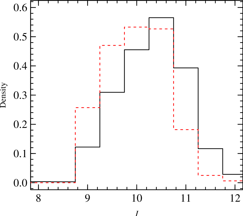
Figure 3.— Distribution of $I$-magnitude for our candidate sample (red-dashed) and the parent RAVE sample (solid-black). Note that the RAVE sample only includes those stars that satisfied our constraints in §2.

4. Abundance Analysis

Initial estimates of the stellar parameters ($T_{\rm ini}$, $\log~{}g_{\rm ini}$, $\rm[Fe/H]_{ini}$) for each star were determined following the methodology of R10, based on the methods of Fulbright (2000, hereafter F00). Full details of this technique can be found in R10. It is important to note, however, that this method computes the initial quantities using one-dimensional, plane-parallel LTE Kurucz model atmospheres.

It is important that we derive accurate stellar parameters since we later use these parameters to determine distances to our stars. Parameters derived by our initial analysis, however, can often show large differences from expected values computed by different methods. For example, Ivans et al. (2001) show, using giants analyzed in the relatively metal-poor ($\rm[Fe/H]\sim-1.2$) globular cluster M5, that the $\log~{}g$ derived by methods similar to our initial analysis is often too low, especially for stars near the RGB-tip. This is in part due to the fact that Fe i (and somewhat Fe ii) can be strongly affected by non-LTE effects, and so the estimate of surface gravity and iron abundance can be quite unreliable, especially in low-gravity giants and metal-poor stars when ionization equilibrium between Fe i and Fe ii is assumed in our initial analysis (Thévenin & Idiart, 1999; Asplund et al., 1999; Mashonkina et al., 2011, Lind, K. & Bergemann, M., private communication). As summarized in R10, we therefore utilized high-resolution spectroscopic data for several globular cluster stars, as well as reanalyzed several F00 RGB stars with good Hipparcos parallaxes, to test the accuracy of our initial stellar parameter analysis (derived from our echelle-based analysis) for the giant stars (RGB and RC/HB) in our sample. Using independent estimates of the stellar parameters for these test cases, we found that the estimates from our initial technique must be systematically corrected to achieve improved accuracy. Using a sample of 28 F00 MS/SG stars, we have also found that the initial parameters for our MS/SG stars must be similarly corrected. In the following sections, we give a full description of the corrections to the stellar parameters for our entire sample.

4.1. Giant Star Parameters

In R10, we provided a brief summary of the corrections needed for the giant stars in our sample. In this section, we give the full description of those corrections. It is important to note that the giant star test samples did not include RC/HB stars, however, since the stellar parameter corrections are independent of the evolutionary state of the giant star, it was assumed in R10 that the RC/HB stars would follow the same corrections as the RGB stars.

We computed a photometric temperature ($T_{\rm phot}$), using the González Hernández & Bonifacio (2009) 2MASS color-temperature transformations, and a ‘bolometric’ gravity ($g_{\rm bol}=4\pi GM\sigma T^{4}/L$) for each globular cluster and F00 RGB star. A photometric temperature was also computed for the stars in our sample that showed low initial reddening ($A_{J}<0.05$, see §5.4). We found in R10 that the offset, $\Delta_{T}=T_{\rm ini}-T_{\rm phot}$, shows different correlations with $\rm[Fe/H]_{ini}$ depending on the initial $T_{\rm ini}$ of the star. The behavior can be well approximated by two regimes, hotter and cooler than 4500 K, with correlations as illustrated in Figures 4 and 5.

A robust least-squares linear fit to the stars with $T_{\rm ini}>4500$ K (see Figure 4) resulted in:

$$\Delta_{T}=\left\{\begin{array}[]{l l}0&\quad{\rm if~{}\rm[Fe/H]_{ini}}\geq-1.0\\ 240~{}\rm[Fe/H]_{ini}+240&\quad{\rm if}-1>\rm[Fe/H]_{ini}\geq-2.5\\ -400&\quad{\rm if~{}\rm[Fe/H]_{ini}}<-2.5\\ \end{array}\right.$$ (1)

while for stars with $T_{\rm ini}\leq 4500$ K (see Figure 5):

$$\Delta_{T}=\left\{\begin{array}[]{l l}0&\quad{\rm if~{}\rm[Fe/H]_{ini}}\geq-1.2\\ 120~{}\rm[Fe/H]_{ini}+140&\quad{\rm if~{}\rm[Fe/H]_{ini}}<-1.2\\ \end{array}\right.$$ (2)

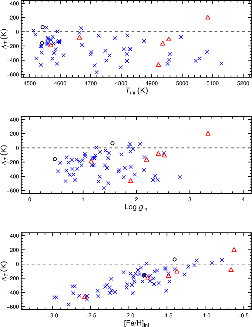
Figure 4.— $\Delta_{T}$ vs. $T_{\rm ini}$, $\log~{}g_{\rm ini}$, and $\rm[Fe/H]_{ini}$ for giant stars with $T_{\rm ini}>4500$ K. Black circles and red triangles represent the globular cluster stars and F00 RGB stars, respectively. The blue x-symbols are giants from our sample that have small initial reddening ($A_{J}<0.05$). Notice that there is no obvious trend with $T_{\rm ini}$ or $\log~{}g_{\rm ini}$, however, it is clear that $T_{\rm ini}-T_{\rm phot}$ depends on $\rm[Fe/H]_{ini}$.

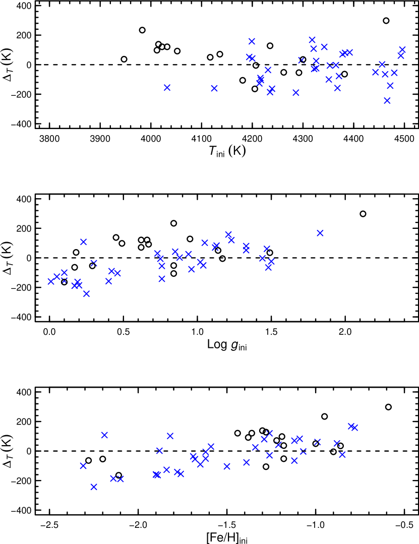
Figure 5.— Same as Figure 4, but only for stars with $T_{\rm ini}\leq 4500$ K. Similarly to Figure 4, the only obvious correlation is with $\rm[Fe/H]_{ini}$. It is important to notice, however, that the slope of the correlation is shallower than for the stars with $T_{\rm ini}>4500$ K. This is the reason we separate the stars into two temperature regimes.

Following the reasoning of R10, we adopted the above corrections, adding $\Delta_{T}$ to $T_{\rm ini}$ to obtain final values for the stellar temperature (denoted as $T_{\rm eff}$), to bring our initial temperatures to a scale that will reduce spurious trends as found for our initial spectroscopic analysis. We then used this final estimate of $T_{\rm eff}$ in the abundance analysis to obtain a new (ionization-balanced) estimate of gravity, denoted $\log~{}g_{\rm phot}$. Comparisons of this $\log~{}g_{\rm phot}$ estimate with $\log~{}g_{\rm bol}$ showed improvement, but an offset still remained for the lowest gravity stars. This residual offset correlates with $\log~{}g_{\rm phot}$ (see Figure 6) such that a least-squares linear fit to the data resulted in:

$$\Delta_{g}=\left\{\begin{array}[]{l l}0.0&\quad{\rm if}~{}\log~{}g_{\rm phot}\geq 1.0\\ 0.6~{}\log~{}g_{\rm phot}-0.6&\quad{\rm if}~{}\log~{}g_{\rm phot}<1.0\\ \end{array}\right.$$ (3)

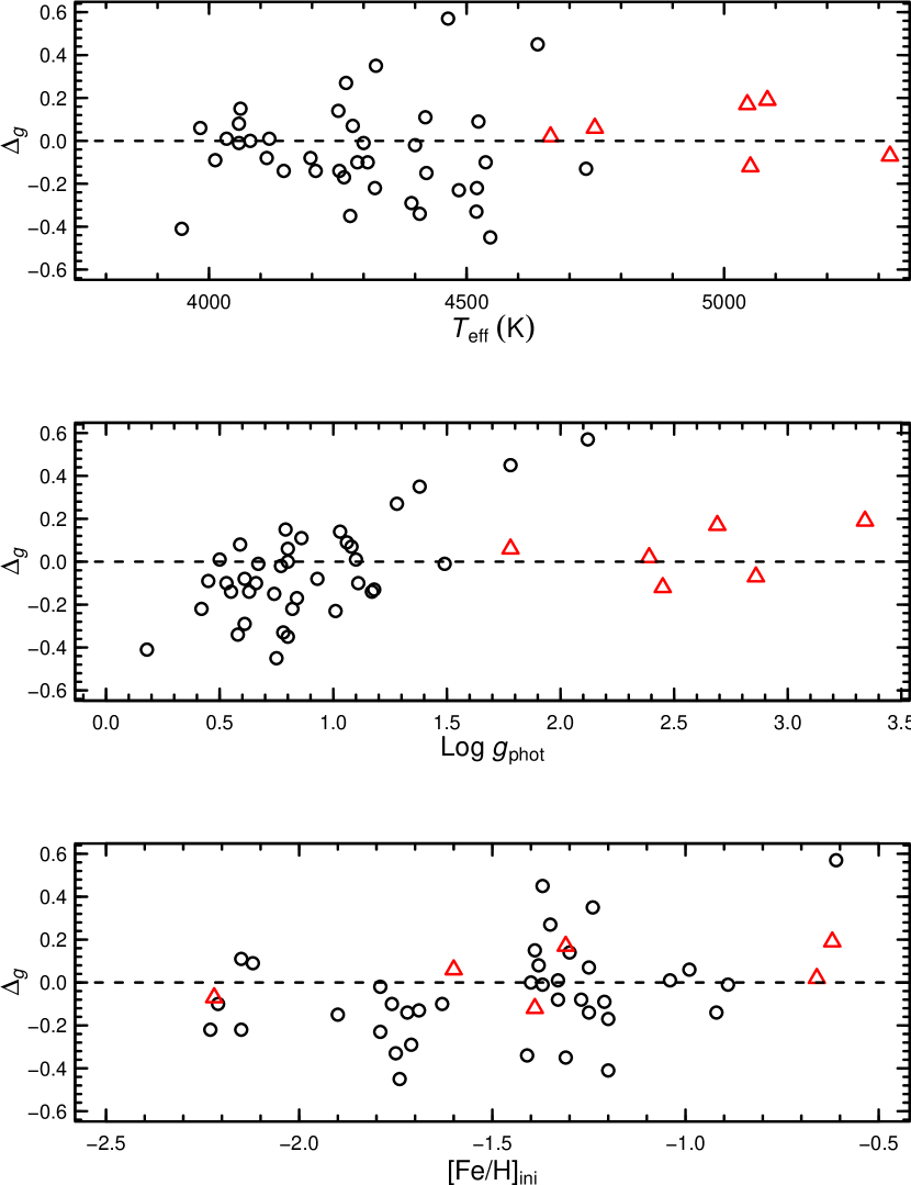
Figure 6.— Difference, $\log~{}g_{\rm phot}-\log~{}g_{\rm bol}$, vs. corrected $T_{\rm eff}$, $\log~{}g_{\rm phot}$, and $\rm[Fe/H]_{ini}$. Black circles and red triangles represent the globular cluster stars and F00 RGB stars, respectively. Notice that after the temperature correction (equations 1 and 2) $\Delta_{g}$ only depends on $\log~{}g_{\rm phot}$.

For those stars with $\log~{}g_{\rm phot}<1$, we applied the above correction to the $\log~{}g_{\rm phot}$ estimate. We then adopted both the corrected $T_{\rm eff}$ and this new $\log~{}g$ estimate to get a new estimate of the iron abundance. We chose the iron abundance from Fe ii as our final estimate of iron abundance to reduce sensitivity to non-LTE effects (Thévenin & Idiart, 1999; Asplund et al., 1999). Scatter from our final estimates of temperature and gravity around $T_{\rm phot}$ and $\log~{}g_{\rm bol}$ provided error estimates, $\sigma_{T_{\rm eff}}=140$ K and $\sigma_{\log~{}g}=0.2$ dex. The iron abundances in the literature are not on a uniform scale, so we estimated the error $\sigma_{\rm[Fe/H]}=0.1$ dex, from star-to-star scatter within any one globular cluster.

4.2. MS/SG Star Parameters

Only the giant stars in our sample were tested in R10. We therefore reanalyzed 28 MS/SG stars from F00 to test the accuracy of the initial stellar parameters for the MS/SG stars in our sample. We computed an independent $\log~{}g_{\rm bol}$ and photometric temperature, $T_{\rm phot}$, following the same methods as for the giants. We also included estimates of photometric temperature for the MS/SG stars in our sample with low initial reddening (as done for the giant stars). We found, through a linear fit to the data, that the offset, $\Delta_{T}=T_{\rm ini}$-$T_{\rm phot}$, correlates with $\rm[Fe/H]_{ini}$ for these stars such that:

$$\Delta_{T}=190~{}\rm[Fe/H]_{ini}+150$$ (4)

This correlation is illustrated in Figure 7. In addition, Figure 8 shows that the difference, $\Delta_{g}=\log~{}g_{\rm ini}-\log~{}g_{\rm bol}$, correlates with both $\rm[Fe/H]_{ini}$ and $\log~{}g_{\rm ini}$ for the MS/SG stars. The linear fit to this correlation is given by:

$$\Delta_{g}=0.3~{}\rm[Fe/H]_{ini}+0.2~{}\log~{}g_{\rm ini}-0.8.$$ (5)

We simultaneously corrected our initial $T_{\rm ini}$ and $\log~{}g_{\rm ini}$ values according to the above correlations, which resulted in mean scatter around $T_{\rm phot}$ and $\log~{}g_{\rm bol}$ of 150 K and 0.2 dex, respectively. Again (as for the giants), we chose the abundance of Fe ii as our final estimate of iron abundance.

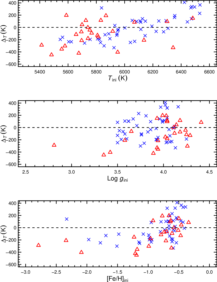
Figure 7.— Difference, $T_{\rm ini}-T_{\rm phot}$, vs. $T_{\rm ini}$, $\log~{}g_{\rm ini}$, and $\rm[Fe/H]_{ini}$ for the 28 MS/SG stars from F00. Red triangles represent the F00 data, while the blue x-symbols represent MS/SG stars in our sample with low initial reddening ($A_{J}<0.05$).

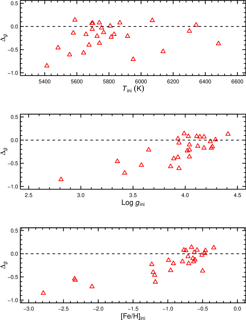
Figure 8.— $\Delta_{g}$ vs. corrected $T_{\rm eff}$, $\log~{}g_{\rm ini}$, and $\rm[Fe/H]_{ini}$ for the F00 MS/SG stars. It is clear from this figure that $\Delta_{g}$ for the MS/SG stars depends on both $\log~{}g_{\rm ini}$ and $\rm[Fe/H]_{ini}$.

4.3. Final Values of Stellar Parameters

We used the above procedures to ensure that the derived parameter values for our candidate metal-poor thick disk sample are on the same scales as the globular cluster stars and Hipparcos stars. Stars with repeat observations showed small differences in the values of the stellar parameters after the corrections above, but they are all smaller than our estimated errors during the correction procedure. The effective temperatures showed mean differences of $16\pm 58$ K, the $\log~{}g$ values differed by $0.05\pm 0.12$ dex, and there was a mean difference of $0.02\pm 0.07$ dex in $\rm[Fe/H]$.

Table 2 gives our final stellar parameter values for our sample. Figure 9 illustrates the position of our stars on the $\log~{}g$ versus $\log(T_{\rm eff})$ plane before (left panel) and after (right panel) the above corrections. Two isochrones, computed by the Padova group (Girardi et al., 2002; Marigo et al., 2008), with an age of 12 Gyr and metallicities $Z=0.001$ and $Z=0.006$ are plotted for reference. Notice that the resulting gravities for the RGB trace the isochrones much better after the corrections. Note that some MS/TO stars have different metallicities than the reference isochrones, which makes them appear to be in an impossible part of the plane.

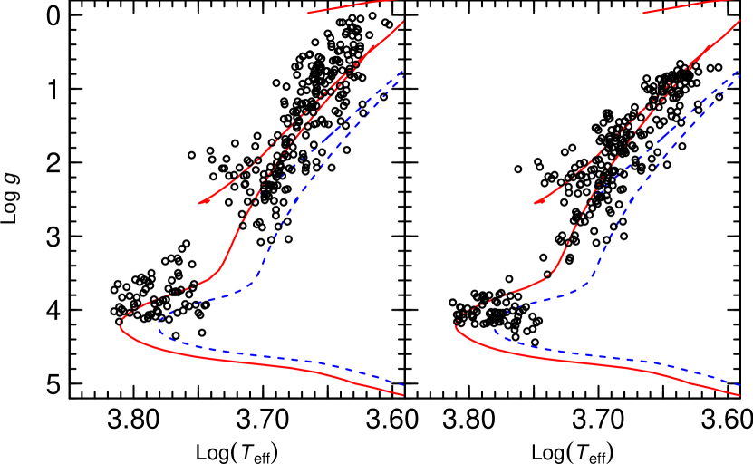
Figure 9.— Stellar positions in the $\log~{}g$ vs. $\log(T_{\rm eff})$ plane before (left panel) and after (right panel) our stellar parameter corrections. The isochrones plotted have an age of 12 Gyr and metallicities $Z=0.001$ (solid red curve) and $Z=0.006$ (dashed blue curve). Some MS/TO stars have different metallicities than the reference isochrones, which makes them appear to be in an impossible part of the plane. See Figure 12 for plots of isochrones more appropriate for the MS/SG stars.

In Figure 10, we compare our stellar parameter values with those from RAVE. As can be seen in the figure, on average the RAVE values for $T_{\rm eff}$ and $\log~{}g$ match the echelle-derived values. There is, however, a large spread, especially for RGB stars at low ($\log~{}g<2$) gravity. The echelle-derived values also tend to have hotter temperatures and larger gravities for the dwarfs and sub-giants. Metallicity comparisons show a tight trend between the difference of the two measurements with the echelle-derived value. It is clear that the RAVE [M/H] is not the same as our echelle-derived $\rm[Fe/H]$.

Figure 10.— Stellar parameter comparisons with RAVE values: $T_{\rm eff}$ (upper left panel), $\log~{}g$ (upper right panel), and metallicity (lower left panel). All panels plot the echelle value of the parameter minus the analogous RAVE parameter versus the echelle value. Note that there is a tight correlation between the difference in metallicity values versus the echelle-derived $\rm[Fe/H]$, which results from the fact that the RAVE [M/H] is the estimated total metallicity from iron and the alpha elements together. The more metal-poor stars are more enhanced in the alpha-elements (shown later), which increases this total metallicity.

4.4. Abundances of the Alpha-Elements

Elemental abundances of several $\alpha$-elements were taken from R10 for the RGB and RC/HB stars, while those for the MS/SG stars were derived using the MOOG analysis program (Sneden, 1973) using the final stellar parameters for each star (as done for the giants in R10). The ratio of the abundance of each $\alpha$-element to iron abundance, computed using solar abundances from Grevesse et al. (1996), can be found in Table 2. Comparisons of repeat observations for each ratio, showed differences of $\lower 2.15277pt\hbox{$\;\buildrel<\over{\sim}\;$}0.03\pm 0.1$ dex. We therefore adopted an error of $0.1$ dex in the $\rm[\alpha/Fe]$ ratios. Final abundance values for stars with repeats were taken as the average of the two estimates for each element.

Table 2Atmospheric and Abundance-Ratio Data

Star	$T_{\rm eff}$ (K)	$\log~{}g$	$\rm[Fe/H]$	$v_{t}$	Mg	Si	Ca	Ti i	Ti ii
C0023306-163143	5528	3.29	-2.30	1.4	0.32	0.46	0.34	0.11	0.15
C0315358-094743	4722	1.77	-1.35	1.6	0.30	0.45	0.28	0.11	0.24
C0408404-462531	4600	0.86	-2.13	2.1	0.42	0.44	0.32	0.09	0.18
C0549576-334007	5379	3.04	-1.76	1.3	0.24	0.22	0.31	0.15	0.21
C1141088-453528	4592	1.01	-2.32	1.9	0.35	0.37	0.28	0.02	0.20

given as [Fe ii/H] given as [X/Fe i] given as [X/Fe ii]

Note. — Table 2 is published in its entirety in the electronic edition of the Astrophysical Journal. A portion is shown here for guidance regarding its form and content.

5. Stellar Distances

For this effort to yield meaningful conclusions, we have to determine meaningful population assignments (see §6). Meaningful population assignments require accurate kinematic values to distinguish the thick disk from the halo and thin disk. The greatest contributor to the uncertainty in the kinematics is the distance uncertainty. We therefore applied techniques that minimized the uncertainty in the derived distances to our stars.

5.1. RGB Stars

Distances to the RGB stars were adopted from R10, in which we utilized a method that determines probability weights for a set of isochrones. An absolute $M_{K_{\rm S}}$ magnitude of a given star was then determined by matching the parameters of a star to the most probable isochrone using the technique described below.

5.1.1 The Isochrones

Throughout the analysis of R10, as well as this work, we used the set of isochrones computed by the Padova group. There are, however, many other isochrone sets available. To test the systematics resulting from using one set of isochrones over another, we also utilized a second set of isochrones, the Yonsei-Yale (Yi et al., 2001; Demarque et al., 2004) isochrones, in the analysis of a small subset of our stars covering the full range of stellar parameters for our entire sample. The distance estimates derived from fitting the test data to each isochrone set resulted in an average difference in distance of about 10% – well inside our experimental error (as will be discussed below). This implies that isochrone differences will not have a noticeable effect on our estimated distances.

The Padova isochrones were chosen for the remainder of our analysis since they can be simply computed for 2MASS magnitudes, and also include the late stages (HB and AGB) of stellar evolution. For the RGB distance analysis, we created a grid (without interpolation) of Padova isochrones with metallicities ranging between $Z=0.0001$ and $Z=0.01$ (with solar elemental ratios) with a step-size of 0.0002, and ages ranging between $4-12$ Gyr with a step-size of 1 Gyr.

5.1.2 The Fit Technique

The technique from R10 fit the stellar parameters of each star to several isochrones. A series of sequential weighted averages over the isochrones were then performed to find the most probable $M_{K_{\rm S}}$ magnitude for each star. Note that we do not perform any interpolation between isochrone grid points. The points along the RGB of each isochrone are approximately uniformly distributed, however, the spacing between points on different isochrones (especially of differing metallicity) can be uneven, which may cause over-sampling or under-sampling of different regions of the entire grid. We attempted to reduce this effect by restricting the range of metallicities used in the fit and introducing a prior probability to each grid point, as described below.

The parameters used to fit each star were $T_{\rm eff}$, $\log~{}g$, and the $Z$-metallicity of the star. The $Z$-metallicity was determined by combining $\rm[Fe/H]$ and the mean $\rm[\alpha/Fe]$ using the prescription of Salaris et al. (1993),

$$Z=Z_{o}(0.638\cdot 10^{-{\rm[\alpha/Fe]}}+0.362),$$ (6)

where $Z_{o}=Z_{\odot}10^{\rm[Fe/H]}$ and $Z_{\odot}=0.019$ is the solar metallicity. Errors in $\rm[Fe/H]$ and $\rm[\alpha/Fe]$ were propagated to estimate the errors in $Z$. Next, the probability distribution of each parameter was assumed to be described by a Gaussian,

$$\mathcal{N}(X_{\star},\sigma_{X_{\star}})~{}\propto~{}\exp[-(X-X_{\star})^{2}/2\sigma_{X_{\star}}^{2}].$$ (7)

The sigmas, $\sigma_{X_{\star}}$, are the estimated errors in each parameter, $X_{\star}=\{T_{\rm eff},~{}\log~{}g,~{}Z\}$, derived for each star in §4. The grid of isochrones were then redefined so that for a single age, the grid is limited to only isochrones with metallicities within $\pm 10$ times the error of a star’s $Z$-metallicity.

In an effort to reduce cases in which two isochrones of differing ages and metallicities might give the same probability, a prior probability function was also introduced. This function, computed for each point in the grid of isochrones, was derived from the BaSTI luminosity function tracks (Pietrinferni et al., 2004). By this method, evolutionary stages with longer lifetimes will be assigned a larger prior probability than short-lived stages, thus biasing the fit to the longer-lived stages (cf. Pont & Eyer, 2004).

The probability information was then combined so that for each point on an isochrone of a given age, $i$, and metallicity, $j$, a probability weight was computed by,

$$P_{ij}(X_{k})=\Psi_{ij}(X_{k})\prod_{X_{\star}}\mathcal{N}(X_{\star},\sigma_{X_{\star}})$$ (8)

where $\mathcal{N}(X_{\star},\sigma_{X_{\star}})$ is given by equation (7), $\Psi_{ij}(X_{k})$ is the prior probability, and $X_{k}$ equals the set of values, $\{T_{\rm eff},~{}\log~{}g,~{}Z\}$, at the given point, $k$, on the isochrone.

The total probability weight for an isochrone of a given age and metallicity was determined by summing all $P_{ij}(X_{k})$ over all $k$ points in the isochrone. Further, the most probable $M_{K_{\rm S}}$ for the given star when matched to that isochrone was computed by performing the weighted average,

$$M_{ij}=\frac{\sum_{k}P_{ij}(X_{k})M_{ij}(X_{k})}{\sum_{k}P_{ij}(X_{k})},$$ (9)

where $M_{ij}$ is the most probable absolute $M_{K_{\rm S}}$ magnitude of the star if it has the age and metallicity of the given isochrone.

Next, the weighted average of the estimates, $M_{ij}$, of absolute magnitude was performed over all $j$-metallicities to give the most probable estimate $M_{i}$ of a given age,

$$M_{i}=\frac{\sum_{j}P_{ij}M_{ij}}{\sum_{j}P_{ij}}.$$ (10)

where $P_{i}=\sum_{j}~{}P_{ij}$ is the total probability weight at $i$-age, summed over all metallicities within the range. Finally, the estimates of the best absolute magnitude, $M_{i}$, obtained for isochrone ages of 10, 11, and 12 Gyr, were combined by a weighted average to produce the final estimate of the absolute magnitude $M_{K_{\rm S}}$ for each star (as used in R10).

5.2. RC/HB Stars

As with the RGB stars, distances to the RC/HB stars were adopted from R10. Mass loss along the RGB, which affects the position of the HB, is not well modeled in the Padova isochrones. The absolute $M_{K_{\rm S}}$ magnitude for each RC/HB star was therefore assumed to be equal to the single HB point on the isochrone of equivalent $Z$-metallicity and ${\rm age}=12$ Gyr.

5.3. MS/SG Stars

Distances determined by fitting near the turn-off (TO) on isochrones are much more sensitive to age determination than on the RGB. In addition, the fit technique for the RGB stars described above can result in unphysical solutions in this region. The percent error in the $T_{\rm eff}$ value of a star is typically much smaller than that of the $\log~{}g$ values, implying the probability distribution close to the TO region can be double-peaked. For example, a star with a gravity that lies to the right of the TO point on an isochrone will have a probability peak on the MS-branch as well as one on the SG-branch. This will cause any weighted averaging of the isochrones to choose the most probable fit to be a point not on the isochrone itself, which is physically impossible. We, therefore, employed a different method for finding distances to our MS/SG stars to reduce this effect.

Instead of fitting to isochrones, we estimated the absolute $M_{K_{\rm S}}$ magnitude by assuming a mass, using the definition of effective temperature and adopting a bolometric correction for each MS/SG star, which is given by:

$$\begin{split}M_{K_{\rm S}}=&-2.5\left(\log\frac{\rm M}{\rm M_{\odot}}\right.\\ &\left.+4\log\frac{T_{\rm eff}}{T_{\odot}}-\log\frac{g}{g_{\odot}}\right)+M_{{\rm bol},\odot}-BC_{K_{\rm S}}\end{split}$$ (11)

where $T_{\odot}=5770$ K, $\log~{}g_{\odot}=4.44$, $M_{{\rm bol},\odot}=4.72$ is the absolute bolometric magnitude of the Sun, and $BC_{K_{\rm S}}$ are the bolometric corrections derived from Masana et al. (2006), which are applicable for the entire metallicity range of our stars and have propagated errors around $\sim 0.05$. This equation, however, still depends on the mass of a star. Investigating the mass ranges around the turn-off on the isochrones shows that MS/SG stars range in mass between $\sim 0.8-1.0$ ${\rm M}_{\odot}$  for ages $4-12$ Gyr. Adopting a mass of 0.8 ${\rm M}_{\odot}$ implies that the star is old, while adopting a mass of 1.0 ${\rm M}_{\odot}$ implies that the star is younger. Comparing a star’s position in the $\log~{}g$ versus $T_{\rm eff}$ plane to a 4 Gyr and 12 Gyr isochrone, we can determine a reasonable mass estimate. This is described in more detail below.

5.4. Reddening

An estimate of the reddening to a given star was computed during the procedure to obtain a distance by the following method. The Schlegel et al. (1998) dust maps and extinction calculator were initially used to calculate reddening to infinity in a specific line-of-sight. Bonifacio et al. (2000) found that Schlegel et al. (1998) overestimate the reddening when $E(B-V)_{Sch}>0.10$ , and 52 of our candidate stars meet this criterion. We therefore adopted their correction for the extinction:

$$\begin{split}E(B-&V)_{C}=\\ &\begin{cases}E(B-V)_{Sch},~{}~{}{\rm if}~{}E(B-V)_{Sch}\leq 0.10\\ 0.10+0.65~{}[E(B-V)_{Sch}-0.10],~{}{\rm otherwise.}\\ \end{cases}\end{split}$$ (12)

where $E(B-V)_{C}$ is the reddening estimate after the correction. Several stars (especially MS/SG stars) are close enough to lie within the Galactic dust distribution, and thus the reddening should be reduced. Adopting a simple exponential model for the dust, with a scale-height of $h=125$ pc (Bonifacio et al., 2000), the reddening to a star at distance $D$ and Galactic longitude $b$ is reduced by a factor $1-\exp(-|D~{}\sin~{}b|/h)$. The reddening was recomputed iteratively until the difference between the current estimate of the distance and the previous one was less than 2 percent. Schlegel et al. (1998) assumed a $R_{V}=3.1$ extinction curve to compute extinction coefficients in other passbands. They do not, however, derive values for the 2MASS passbands. We determined our extinction coefficients by assuming the extinction coefficients from McCall (2004),

$$\begin{array}[]{l l}A_{J}&=0.819~{}E(B-V)_{C}\\ A_{K_{\rm S}}&=0.350~{}E(B-V)_{C}.\\ \end{array}$$ (13)

The mean values of $A_{J}$ and $A_{K_{\rm S}}$ for our sample are both less than 0.1, with errors less than 0.1 mag. An error of 0.1 mag in reddening will only cause a $\sim 4\%$ shift in distance, which is within our error estimates described below.

5.5. Comparisons & Error Analysis

We adopted the estimate of 20% error on the distance to RGB and RC/HB stars from R10, which was based on comparisons between our estimates and literature estimates for the globular cluster stars and estimates for the F00 RGB stars derived from Hipparcos parallaxes. For the MS/SG stars, we applied our technique from above to estimate distances for each of the 28 F00 MS/SG stars, and compared to the Hipparcos distances. Figure 11 plots these stars in the $\log~{}g$ versus $\log(T_{\rm eff})$ plane. The majority of the stars appear to be old. There are, however, several stars with $\rm[Fe/H]>-0.6$ that could have younger ages. If we assume all of the stars are old, and choose a mass of 0.8 ${\rm M}_{\odot}$, then the distance estimates from our technique differ from those derived from the Hipparcos parallaxes by only $1\%\pm 17\%$. Increasing the mass to 0.9 ${\rm M}_{\odot}$ and 1.0 ${\rm M}_{\odot}$ increases the difference to $7\%\pm 18\%$ and $13\%\pm 19\%$, respectively. It is important to notice that if we increase the mass to one that is intermediate between older and younger ages, then the difference only increases by 6%, which is well within the scatter.

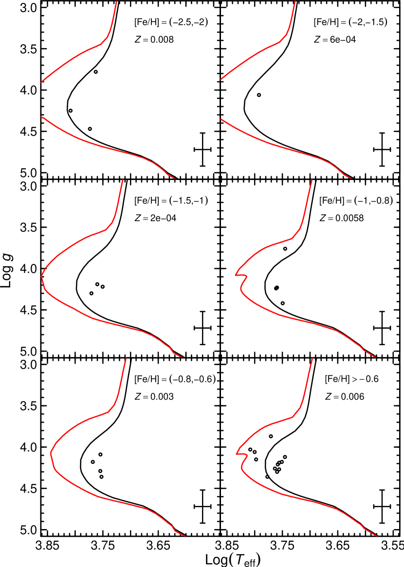
Figure 11.— Plot of $\log~{}g$ vs. $\log(T_{\rm eff})$ for the F00 MS/SG stars (after all parameter corrections) for different metallicity bins as shown in each panel. In addition two isochrone curves are plotted (for the given $Z$-metallicity shown in each panel). The black curve and red curve represent ages of 12 Gyr and 4 Gyr, respectively. Note that the majority of the F00 stars appear to be old, except for a few with $\rm[Fe/H]>-0.6$.

Figure 12 shows the same plots as Figure 11, except we now plot our metal-poor sample MS/SG stars. It is clear that all stars with $\rm[Fe/H]<-1$ are old. We therefore assume they have a mass of 0.8 ${\rm M}_{\odot}$. We assume a mass of 1.0 ${\rm M}_{\odot}$ for the two stars with $\rm[Fe/H]=(-1,-0.8)$ close to the 4 Gyr isochrone ($\log(T_{\rm eff})>3.78$), while we adopt 0.8 ${\rm M}_{\odot}$ for the remaining stars in that bin. Those stars with $\rm[Fe/H]>-0.8$ show no clear separation in age. We therefore chose an intermediate mass of 0.9 ${\rm M}_{\odot}$ for all MS/SG stars with $\rm[Fe/H]>-0.8$. If we apply the above prescriptions to the F00 MS/SG stars, we find a difference between our bolometric distances and the distances derived from parallaxes to be only $4\%\pm 17\%$. We therefore adopt a 20% error on the distances to our MS/SG stars (similarly to the giants and RC/HB stars), so as to include both offsets and scatter.

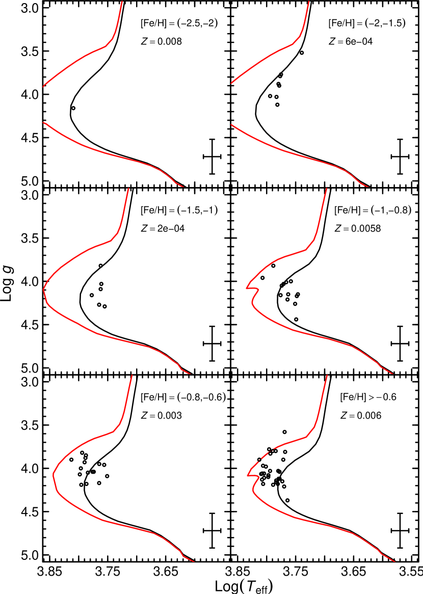
Figure 12.— Plot of $\log~{}g$ vs. $\log(T_{\rm eff})$ for the MS/SG stars in our metal-poor sample (after all parameter corrections) for different metallicity bins as shown in each panel. The isochrones and bins are the same as those in Figure 11. Stars with $\rm[Fe/H]<-0.8$ are all old, except for two younger stars in the $\rm[Fe/H]=(-1,-0.8)$ bin. We therefore assume a mass of 1.0 ${\rm M}_{\odot}$ for the two younger stars, while the remaining stars with $\rm[Fe/H]<-0.8$ are assumed to have a mass of 0.8 ${\rm M}_{\odot}$. The ages of stars with $\rm[Fe/H]>-0.8$ are unclear, and cannot be easily separated. We therefore adopt a mass estimate of 0.9 ${\rm M}_{\odot}$ for these stars.

Distance estimates based on RAVE pipeline values of stellar parameters are also now available (Breddels et al., 2010; Zwitter et al., 2010; Burnett & Binney, 2010). Our distance estimates for the 172 giant stars with $|\log~{}g_{\rm echelle}-\log~{}g_{\rm RAVE}|<0.5$ are shorter than those of Zwitter et al. (2010) by $15\%\pm 24\%$, while the 73 MS/SG stars have distances shorter by $36\%\pm 21\%$. Note that our technique was optimized for metal-poor stars and uses parameters derived from echelle spectra, while Zwitter et al. (2010) optimized their method for all stars in the RAVE catalog, which have a high mean metallicity and typically younger ages and used parameter values from the RAVE pipeline analysis.

5.6. Final Distances

Our final estimate of the distance to each star, from the Sun, can be found in Table 3, with the error being 20% of the distance estimate. The average distance to the RGB and RC/HB stars is $\sim 2$ kpc. All had distances less than $\sim 7$ kpc, except one at $\sim 16$ kpc (see Figure 13). The MS/SG stars in our sample have an average distance of $\sim 220$ pc, extending out to $\sim 400$ pc. The majority of our stars (primarily giants) extend to an average vertical height of $|z|\lower 2.15277pt\hbox{$\;\buildrel>\over{\sim}\;$}1$ kpc, as shown in Figure 13. It is clear that our sample probes distances much further than the solar neighborhood ($\sim 100$ pc) – not done by any previous analyses of elemental abundances of metal-poor thick disk stars in the literature.

Figure 13.— Distribution of total distance (upper panel) and vertical $|z|$-height (lower panel) for our candidate sample. Note that the star at a distance of $\sim 16$ kpc is not shown.

5.7. Velocities and Orbits

We computed three-dimensional space motions of our stars in cylindrical coordinates (given in Table 3) by combining the distances and radial velocities derived from the analysis of our spectra with the proper motions given in the RAVE database. We further derived the full orbit of each star by assuming a Galactic potential and combining that with the velocity and position information for each star. Stellar orbits were computed over 15 Gyr using an orbital integrator based on a three-component Galactic potential. The disk is modeled as a Miyamoto-Nagai potential (Miyamoto & Nagai, 1975), while we used the Hernquist (1990) potential for the bulge. Finally, we assumed a logarithmic spherical potential for the halo. We took $M_{\rm disk}=8.0~{}{\rm x}~{}10^{10}$ ${\rm M}_{\odot}$, $M_{\rm bulge}=2.5~{}{\rm x}~{}10^{10}$ ${\rm M}_{\odot}$, with characteristic scales $a=6.5$, $b=0.26$, $c=0.7$, and $d=12.0$, all in kiloparsecs, and $v^{2}_{\rm halo}=27000\,({\rm km~{}s^{-1}})^{2}$. These values ensure that the circular velocity equals 220 ${\rm km~{}s^{-1}}$ at 8 kpc from the Galactic center.

The orbital parameters of each star are listed in Table 4. Two sets of data are listed. The maximum vertical distance, $|z_{max}|$, and the closest and furthest distances,$r_{\rm per}$ and $r_{\rm apo}$, reached by a star for all orbits integrated are listed in columns 3 through 5, while the same parameters for the final orbit of the star are listed in columns 6 through 8. The total number of orbits integrated is given as $N_{\rm orbit}$. The eccentricity of any given orbit of a star is defined as

$$\varepsilon=\frac{r_{\rm apo}-r_{\rm per}}{r_{\rm apo}+r_{\rm per}}.$$ (14)

The parameters for the last orbit were chosen to compute $\varepsilon$ in order to make direct comparisons of stellar eccentricities with model simulations (see §9). The amplitude of variation for $r_{\rm per}$ and $r_{\rm apo}$ depends on the $z$-excursions during each orbit of a star, and thus, can be quite large. The amplitude of variation in the eccentricity of an orbit, however, is typically less than 0.05. We therefore assume the eccentricity of the last orbit is representative of the true orbital eccentricity of a star.

Table 3Kinematic Data

Star	$D$	$V_{\rm helio}$	$V_{\Pi}$	$\epsilon_{\Pi}$	$V_{\Theta}$	$\epsilon_{\Theta}$	$V_{Z}$	$\epsilon_{Z}$	$P_{\rm thin}$	$P_{\rm thick}$	$P_{\rm halo}$	POP
	(pc)	(${\rm km~{}s^{-1}}$)	(${\rm km~{}s^{-1}}$)	(${\rm km~{}s^{-1}}$)	(${\rm km~{}s^{-1}}$)	(${\rm km~{}s^{-1}}$)	(${\rm km~{}s^{-1}}$)	(${\rm km~{}s^{-1}}$)
C0023306-163143	921	-7.0	53.2	19.3	-195.3	85.9	-77.9	19.0	0.00	0.00	1.00	3
C0315358-094743	2434	131.6	86.3	14.6	50.4	36.4	-54.0	15.2	0.00	0.13	0.87	3
C0408404-462531	15699	52.3	74.2	344.8	-88.9	338.4	241.7	269.9	0.00	0.01	0.99	3
C0549576-334007	1157	79.7	-29.1	16.4	134.6	11.7	-24.7	14.2	0.02	0.91	0.07	2
C1141088-453528	6152	83.9	-105.0	54.2	58.1	51.9	-88.1	69.2	0.00	0.11	0.89	3

Note. — Table 3 is published in its entirety in the electronic edition of the Astrophysical Journal. A portion is shown here for guidance regarding its form and content.

Table 4Orbital Parameters

		All Orbits			Final Orbit
Star	${\rm N_{orbit}}$	$r_{\rm per}$	$r_{\rm apo}$	$|z_{\rm max}|$	$r_{\rm per}$	$r_{\rm apo}$	$|z_{\rm max}|$	$\varepsilon$
		(kpc)	(kpc)	(kpc)	(kpc)	(kpc)	(kpc)
C0023306-163143	100	6.5	9.2	1.6	6.6	9.1	1.5	0.2
C0315358-094743	116	1.4	10.6	2.3	1.6	10.5	2.2	0.7
C0408404-462531	61	15.9	23.8	23.8	16.9	23.5	23.4	0.2
C0549576-334007	119	3.9	8.9	0.6	3.9	8.9	0.6	0.4
C1141088-453528	127	0.6	10.6	3.4	0.7	9.8	2.4	0.9

Note. — Table 4 is published in its entirety in the electronic edition of the Astrophysical Journal. A portion is shown here for guidance regarding its form and content.

6. Population Assignments

Each star was assigned to a Galactic population following the same Monte-Carlo method as in R10. We drew 10,000 random samples of each component of a star’s space motion from a Gaussian error distribution centered on our estimate of the component velocity. The probabilities that each random set of velocities was drawn from the thin disk, thick disk, or halo were then computed using the local characteristic Gaussian definitions for each Galactic population (given in Table 1 of R10 and reproduced here in Table 5). A random set was assigned to a specific Galactic population if the probability was four times that of the other two probabilities. A star was then finally assigned to the Galactic population with the most random set assignments.

It is important to note that some stars had probabilities that did not easily distinguish between the Galactic populations (the ratio of the probabilities of two Galactic components was less than four). These stars were then assigned to additional intermediate thin/thick or thick/halo populations. This method, however, is susceptible to possible misassignments. During the analysis, we therefore retained an additional probability statistic. which equalled the sum of the probabilities (normalized) obtained from all Monte-Carlo realizations for each Galactic population (hereafter, the PDF values).

Similarly, random sets of a star’s distance were drawn from a Gaussian error distribution centered on our estimate of the distance and a sigma equal to 20 percent of the distance. The probability that a random ‘star’ lies in each Galactic population was computed by comparing to the characteristic double-exponential distributions for the thin and thick disks and the two-axial power-law ellipsoid for the halo, taken from Jurić et al. (2008). As with the velocities, a star was assigned to the Galactic population with the highest number of occurrences from the re-sampled distance. The positional assignment was then used as a boundary condition such that if a star was assigned to the thick disk from its velocities and it was assigned to the halo from its position, the star would then be assigned to the halo. A star would remain assigned to the thick disk, however, if it was assigned to the thin disk from its position.

Table 5Local Characteristic Velocity Distributions

Population	$\sigma_{\Pi}$	$\sigma_{\Theta}$	$\sigma_{Z}$	$\langle V_{\Theta}\rangle$	Ref.
	(${\rm km~{}s^{-1}}$)	(${\rm km~{}s^{-1}}$)	(${\rm km~{}s^{-1}}$)	(${\rm km~{}s^{-1}}$)
Thin Disk	39	20	20	-15	Soubiran et al. (2003)
Thick Disk	63	39	39	-51	Soubiran et al. (2003)
Halo	141	106	94	-220	Chiba & Beers (2000)

The stars were assigned as follows: 88 thick disk, 21 thin disk, 51 intermediate thin/thick disk, 36 intermediate thick/halo, and 123 halo. The last four columns of Table 3 gives the PDF values and Galactic population assignment for each star. A Toomre diagram is plotted in Figure 14 to illustrate the relationship between our final population assignments and stellar velocities. Note that comparisons with the Toomre diagram from R10 show that the MS/SG stars mainly comprise the thin disk and thin/thick population. We further sum the stars’ PDF values for each Galactic population within a given velocity bin and plot the distribution of each velocity component in Figure 15. It is clear that the distributions reflect the underlying assumed populations.

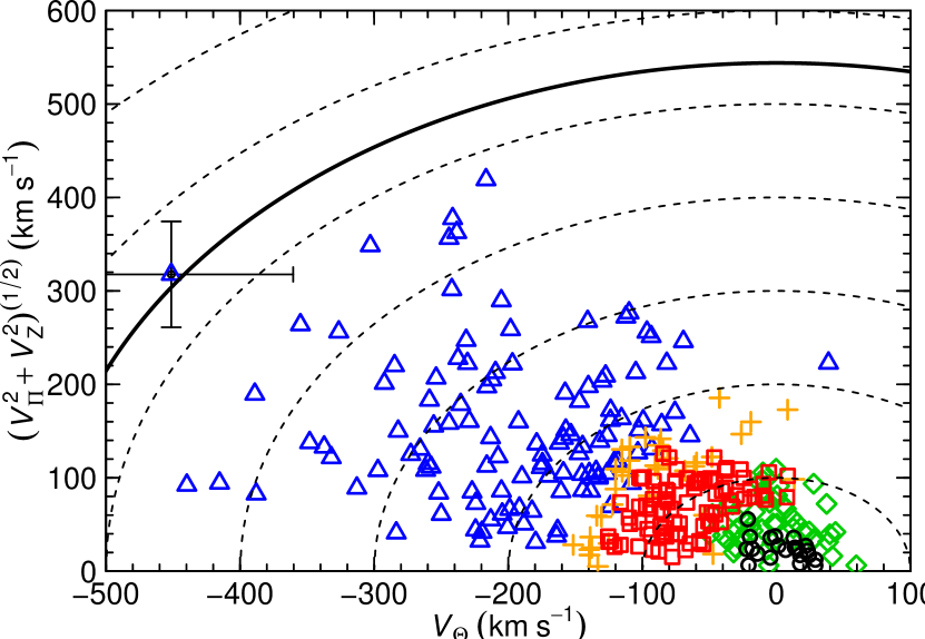
Figure 14.— Toomre diagram for our full sample with $\sigma_{V_{\theta}}<100$ ${\rm km~{}s^{-1}}$. The black circles, green diamonds, red squares, orange plus signs, and blue triangles correspond to thin disk, thin/thick, thick disk, thick/halo, and halo stars, respectively. The dashed curves indicate constant space motion, while an estimate of the local escape velocity, based on radial velocities within the RAVE database (Smith et al., 2007), is represented by the thick solid curve. Typical velocity errors are $1\sigma$ error $<20$ ${\rm km~{}s^{-1}}$.

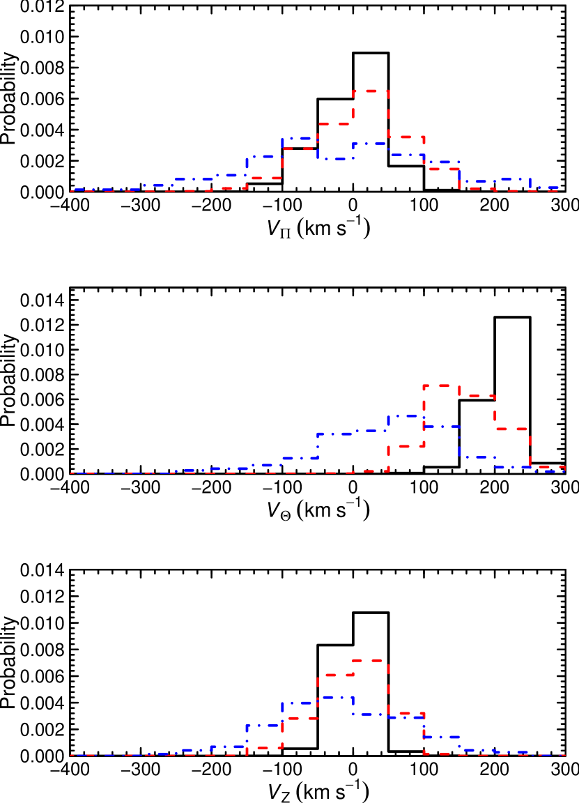
Figure 15.— Distribution of $V_{\Pi}$ (top panel), $V_{\Theta}$ (middle panel), and $V_{Z}$ (bottom panel) velocities for our stars given the PDF value that they belong to the thin disk (solid black), thick disk (dashed red), and halo (dot-dashed blue). Note that each distribution was created by summing the PDF values within a given velocity bin. The distributions were then normalized such that the total area equals unity.

7. The Metal-Poor Thick Disk

7.1. Iron Abundance Distribution and Gradients

Recall (from §4) that we estimate the iron abundance of each star from Fe ii, since Fe ii is both the dominant species and is much less sensitive to non-LTE effects than is Fe i (Thévenin & Idiart, 1999; Asplund et al., 1999; Mashonkina et al., 2011). Figure 16 shows the PDF values for each Galactic population versus $\rm[Fe/H]$, while Figure 17 shows the distribution of iron abundance for each of the three Galactic populations. As was found in R10, the majority of the thick disk has $\rm[Fe/H]>-1.8$, with a small tail to much lower metallicities, the lowest metallicity being $\rm[Fe/H]\sim-2.7$. The MS/SG stars assigned to the thick disk predominantly have metallicities close to -1 dex, with a short tail down to $\rm[Fe/H]\sim-1.8$. The distribution of $\rm[Fe/H]$, therefore did not show a significant change from that of R10. Due to sample selection effects, we do not completely sample the high-metallicity ($\rm[Fe/H]>-1$) parts of the distributions. Further, the offset between our final $\rm[Fe/H]$ values and the RAVE metallicities (see Figure 10) contributed to the shortage of thick disk stars with metallicities at the peak from local studies ($\rm[Fe/H]\sim-0.6$). Stars that may have seemed to have metallicities near -0.6 dex, would end up with a lower value for the final metallicities.

Figure 16.— PDF values for each Galactic population versus $\rm[Fe/H]$.

The most notable attribute of the thick disk metallicity distribution is that it appears to be double-peaked. The second, low-metallicity peak is comprised of many stars that have intermediate probabilities for both the thick disk and halo (${\rm PDFs}<0.6$, assigned as thick/halo), while the peak above $\rm[Fe/H]\sim-1$ is comprised of stars with probabilities of being thick disk equal to $0.6-1.0$ (see Figure 16). It is therefore important to note that the low-metallicity peak is not just systematic noise in the population assignments, but is actually different. Could this be a metal-poor ‘sub-component’ of the thick disk, or could it be the high angular momentum tail of the halo? We will come back to this later (see §7.3).

Figure 17.— Distribution of $\rm[Fe/H]$ for thin disk, thick disk, and halo. Note that each distribution was created by summing the PDF values within a given metallicity bin. The distributions were then normalized such that the total area equals unity. Recall that our sample was selected to be metal-poor, so that the full metallicity distributions of each component are not uniformly represented.

Before we can determine the presence of iron abundance gradients in the thick disk, we must first determine possible selection effects in our sample and introduced through the analysis. For example, we introduced a temperature cut, such that only stars with temperatures in the range $4000-6500$ K were selected for observation, to reduce contamination of stars that would most likely fail our abundance analysis (see §2). Figure 18 plots $\rm[Fe/H]$ versus $R$ and $|z|$ for our sample on top of the RAVE catalog, with ${\rm[M/H]}<-0.5$, from which our sample stars were selected. We performed a linear fit to the $\rm[Fe/H]$ vs. $\rm[Fe/H]-\rm[M/H]$ relation in Figure 10 in order to put our sample stars and the RAVE catalog stars on the same scale. Distances to the RAVE catalog stars were computed using an analogous method to that described in §5. Our sample does not show the same distance coverage as the RAVE catalog stars for $\rm[Fe/H]\geq-1.2$. This implies that the lack of thick-disk stars with $\rm[Fe/H]\geq-1.2$ at large radial and vertical distances is possibly an artifact of our cuts in temperature.

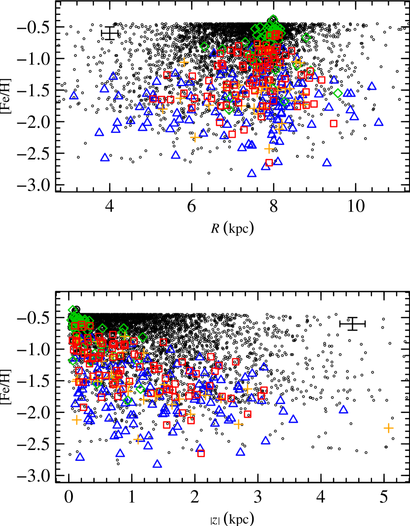
Figure 18.— $\rm[Fe/H]$ vs. $R$ and $|z|$ for our sample of stars (symbols and colors are the same as Figure 14). The small data points are those stars from our original RAVE catalog, from which our sample was taken. The RAVE catalog stars populate large $|z|$, even at high $\rm[Fe/H]$, which suggests that the lack of stars in our metal-poor sample with $\rm[Fe/H]>-1$ at large $|z|$ is due to the selection function of the sample, combined with the subsequent temperature cuts prior to the abundance analysis.

We investigated the possible origin of these selection effects by comparing to an old (12 Gyr) isochrone. In Figure 19, we plot the derived data for our sample together with 12 Gyr isochrones of differing metallicities. The metallicities of the isochrones were simply converted to $\rm[Fe/H]$ by $\rm[Fe/H]=\log({\it Z/Z}_{\odot})$ as a first-order approximation. We applied an apparent magnitude limit of $I=10$, the peak $I$-magnitude of our sample (see Figure 3), to the isochrone data to determine the maximum distance that can be observed for each metallicity. It is clear that the stars of our sample do not reach the maximum limit (as shown in the top panel of Figure 19). However, when we apply the same temperature cut that we applied during our candidate selection ($4000-6500$ K) to the isochrone data, then we see a similar trend emerge in the isochrone behavior as in the sample (lower panel, Figure 19). This is a clear illustration of the selection effects in our final sample. For $\rm[Fe/H]<-1.2$, however, the isochrone data are unaffected by the temperature cut, suggesting that below this value the data for our sample may be used without further corrections.

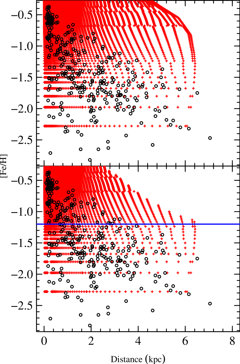
Figure 19.— $\rm[Fe/H]$ vs. Distance for our sample of stars. The red ‘plus’ symbols represent a 12 Gyr isochrone of varying metallicity, for which distances are computed assuming an apparent magnitude of $I=10$. The black points represent our sample of candidate metal-poor thick disk stars. Note that there is one star not shown at a distance of 15 kpc with $\rm[Fe/H]\sim-2.2$. The top panel shows the isochrone points without any temperature cut, while the same temperature cut as that of our candidate sample ($4000-6500$ K) is applied to the isochrone data in the bottom panel. The brightest metal-rich giants are cooler than their metal-poor counterparts, and so the low-temperature limit cuts them out and makes the difference in isochrones seen in the two panels. For $\rm[Fe/H]<-1.2$ (blue line) the sample is unaffected by our temperature cut.

Only the 49 stars assigned to the thick disk with $\rm[Fe/H]<-1.2$ were used to assess the amplitude of metallicity gradients in our metal-poor thick-disk sample, as shown in Figure 20. This figure shows the robust least squares fits to the data along with 95% (2 sigma) confidence intervals for each fit. Both fits have slopes which are formally non-zero, but not significant, corresponding to a $-0.09\pm 0.05~{}{\rm dex~{}kpc}^{-1}$ gradient in the vertical direction and a $+0.01\pm 0.04~{}{\rm dex~{}kpc}^{-1}$ gradient in the radial direction. Iron abundance versus $|z_{\rm max}|$ and $r_{\rm apo}$ (values are maxima for all integrated orbits) also exhibits similar gradients (see Figure 21).

As stated previously, the population assignments are susceptible to possible misassignments. We therefore checked our results using our PDF values. The metallicity with the maximum sum of thick-disk PDFs inside a specific velocity bin was chosen as the metallicity in that given bin. We then fit a line across the maxima to determine possible gradients. The results showed very similar results are very similar to those found using only stars assigned to the thick disk.

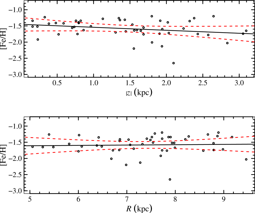
Figure 20.— $\rm[Fe/H]$ vs. $R$ and $|z|$ for stars only assigned to the thick disk (with $\rm[Fe/H]<-1.2$) that are not biased by our selection effects, represented as the black points. Typical errors are $\sim 0.1$ kpc in $R$ and $|z|$ and 0.1 dex in the $\rm[\alpha/Fe]$ ratios. The black line is the robust least squares fit to the data, while the red-dashed curves represent the 95-percentile confidence intervals for the fit. Note that a slope equal to zero (no gradient) is consistent with our data for both $R$ and $|z|$.

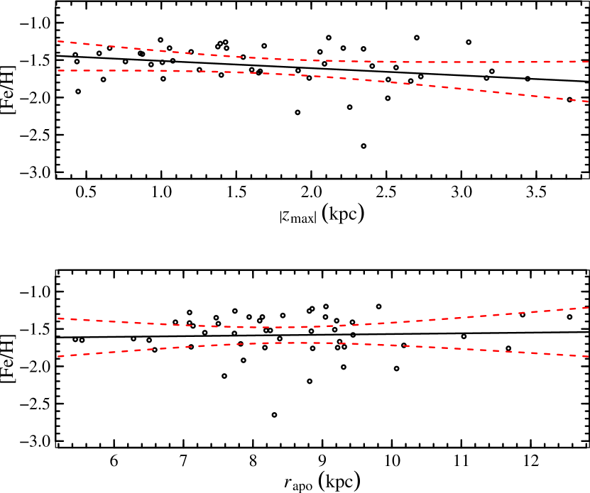
Figure 21.— $\rm[Fe/H]$ vs. $r_{\rm apo}$ and $|z_{\rm max}|$ (columns 4 and 5 of Table 4) for stars assigned to the thick disk with $\rm[Fe/H]<-1.2$. Typical errors are $\sim 0.1$ kpc in $r_{\rm apo}$ and $|z_{\rm max}|$ and 0.1 dex in the $\rm[\alpha/Fe]$ ratios. The black line is the robust least squares fit to the data, while the red-dashed curves represent the 95-percentile confidence intervals for the fit.

It is important to note that at low iron abundance and large distances we are hindered by small-number statistics for the thick disk. We therefore set up a bootstrap analysis, in which we created 10,000 re-samples consisting of 25 stars randomly selected from the 49 stars assigned to thick disk with $\rm[Fe/H]<-1.2$. We performed a least squares fit to each re-sample, and then took the average and standard deviation of all resamples to determine the range to which the fit is affected by possible outliers.

Figure 22 shows the results from this test. The confidence intervals shown in this figure represent the degree to which the fit changes for different random samples. The mean slopes are now only slightly steeper than for our original fits, giving a vertical gradient of $-0.13\pm 0.07~{}{\rm dex~{}kpc}^{-1}$ and a $+0.06\pm 0.06~{}{\rm dex~{}kpc}^{-1}$ radial gradient. Similarly to our original fits, a slope equal to zero is also still consistent within errors.

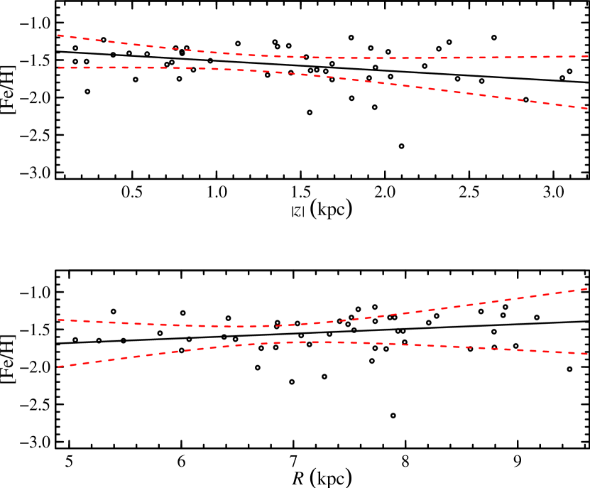
Figure 22.— $\rm[Fe/H]$ vs. $R$ and $|z|$ for stars assigned to the thick disk (with $\rm[Fe/H]<-1.2$). The black lines are now the mean of least squares fits to 10,000 random samples, consisting of only half of the stars assigned to the thick disk. The red-dashed curves represent the 95% confidence intervals derived from the scatter in the distribution of linear fits to each random sample.

7.2. Alpha-to-Iron Ratios

Figure 23 displays several $\rm[\alpha/Fe]$ ratios versus $\rm[Fe/H]$ for our entire sample, which can be directly compared to the same plots in R10 for only the giant stars. Most of the stars with $\rm[Fe/H]>-0.7$ consist of MS/SG stars that were assigned to either the thin disk or thin/thick population, and have an $\alpha$-enhancement lower than for the stars at lower metallicities. The more metal-poor MS/SG stars, however, typically have similar $\alpha$-enhancement to the giants of the same metallicity, an indication that the results from R10 were not affected by the addition of the MS/SG stars.

The metal-poor thick-disk stars have $\rm[\alpha/Fe]$ significantly above solar, $\sim 0.36$ dex for Mg and Si and $\sim 0.27$ dex for Ca and Ti ii. The mean [Ti i/Fe] value is about a tenth of a dex lower than that for Ti ii. This offset is most likely due to non-LTE effects present within our analysis (see Bergemann, 2011). The ratios also show low scatter, $\lower 2.15277pt\hbox{$\;\buildrel<\over{\sim}\;$}0.09$ dex for all $\alpha$-elements, which is less than the 0.1 dex experimental error in $\rm[\alpha/Fe]$. The $\rm[\alpha/Fe]$ ratios also blend smoothly into the halo stars with the difference in mean $\rm[\alpha/Fe]$ ranging between $0.00-0.03$ dex, well within our experimental error. There are a few thick-disk stars with $\rm[Fe/H]>-0.7$ that may have lower enhancement than the metal-poor thick-disk stars, but they do not represent a large enough sample to make any clear conclusion. Also note that, as was shown in R10, there is a thick disk star at $\rm[Fe/H]\sim-1$ with very large [Si/Fe] enhancement and a halo star at $\rm[Fe/H]\sim-1.45$ that shows consistently low $\alpha$-enhancement. These stars, however, show no peculiarities in their kinematics, and will be the subject of future papers.

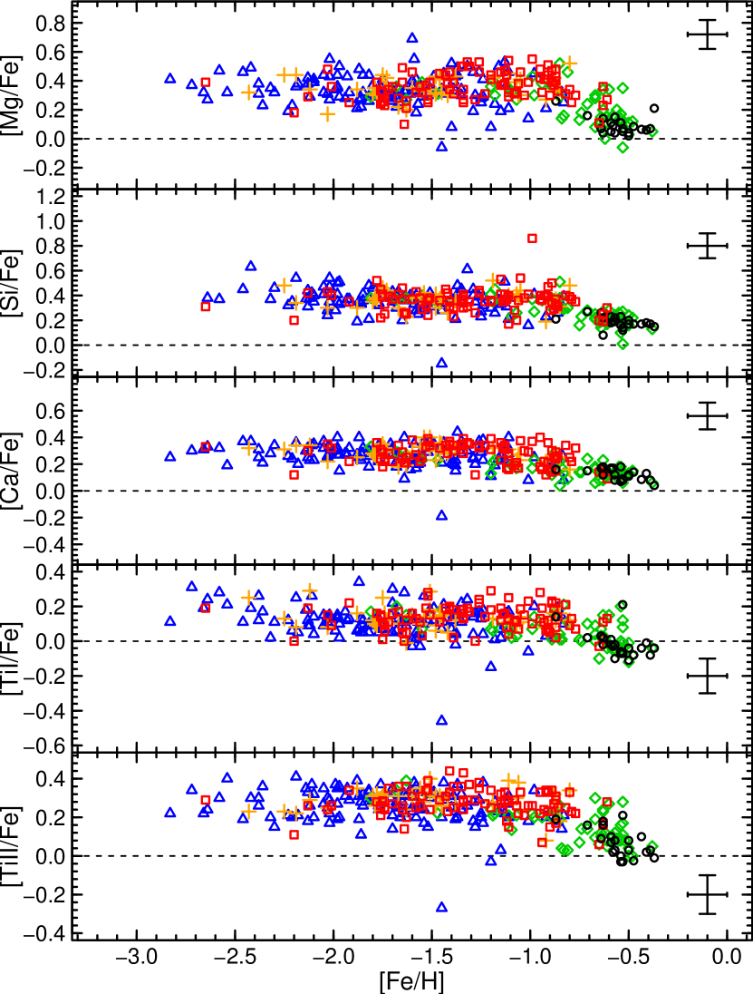
Figure 23.— Computed $\rm[\alpha/Fe]$ ratios vs. $\rm[Fe/H]$ for our sample. Note that element ratios are computed using the iron abundance of the same ionization state as the $\alpha$-element (e.g., [Si/Fe] = [Si i/Fe i]) as is suggested by Kraft & Ivans (2003). Color and symbols are the same as in Fig. 14. The cause of the offset between [Ti i/Fe] and [Ti ii/Fe] is most likely non-LTE effects present within the abundance analysis, but the thick disk and halo still show similar enhancement in each.

Figures 24 and 25 show the $\rm[\alpha/Fe]$ ratios versus $R$ and $|z|$, respectively, for only stars with $\rm[Fe/H]<-1.2$. In both plots, the stars assigned to the thick disk show little dependence on position, for all $\alpha$-elements. In the vertical direction, [Mg/Fe] and [Si/Fe] slightly increase towards larger $|z|$ at $+0.03\pm 0.02~{}{\rm dex~{}kpc}^{-1}$ and $+0.02\pm 0.01~{}{\rm dex~{}kpc}^{-1}$, respectively, while [Ca/Fe] decreases at a rate of $-0.01\pm 0.01~{}{\rm dex~{}kpc}^{-1}$ and [Ti i/Fe] and [Ti ii/Fe] decrease at a rate of $-0.02\pm 0.02~{}{\rm dex~{}kpc}^{-1}$. The ratio of all five elements to iron increase at less than $0.03\pm 0.01~{}{\rm dex~{}kpc}^{-1}$ radially outward. As in the case of iron abundance, the $\rm[\alpha/Fe]$ ratios versus $r_{\rm apo}$ and $|z_{\rm max}|$ show similar gradients (see Figures 26 and 27), only shifting by $\lower 2.15277pt\hbox{$\;\buildrel<\over{\sim}\;$}0.01~{}{\rm dex~{}kpc}^{-1}$ vertically. In addition, the radial gradient reduced to $\sim 0.01~{}{\rm dex~{}kpc}^{-1}$ for all $\alpha$-elements.

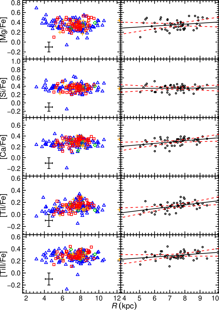
Figure 24.— Computed $\rm[\alpha/Fe]$ ratios vs. $R$ for our sample of stars with $\rm[Fe/H]<-1.2$. The left plots show all populations with symbols and colors the same as Figure 23. The right plots show the least squares fits to only stars assigned to the thick disk. The black line is the fit, while the red-dashed curves represent the 95% confidence intervals.

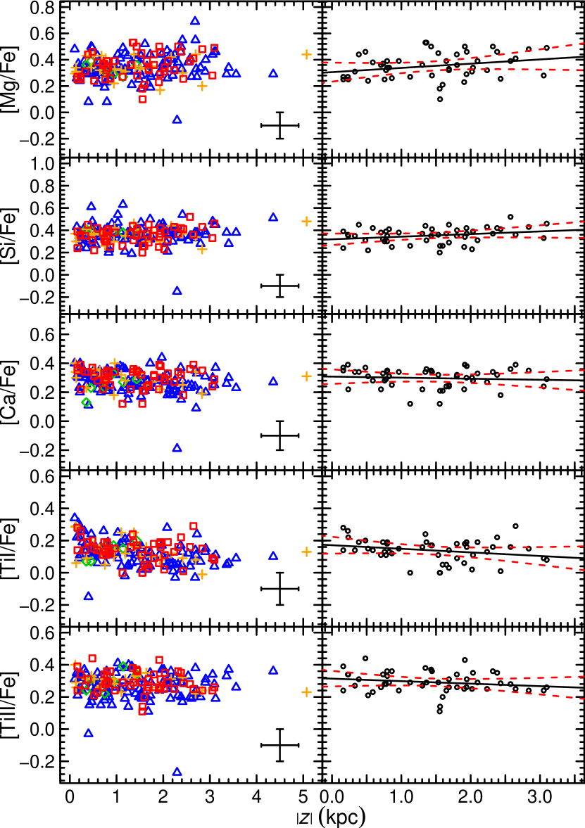
Figure 25.— Computed $\rm[\alpha/Fe]$ ratios vs. $|z|$ for our sample of stars with $\rm[Fe/H]<-1.2$. Symbols and colors are the same as Figure 24. Recall that the left-hand side shows all populations, while the right-hand side shows only the stars assigned to the thick disk.

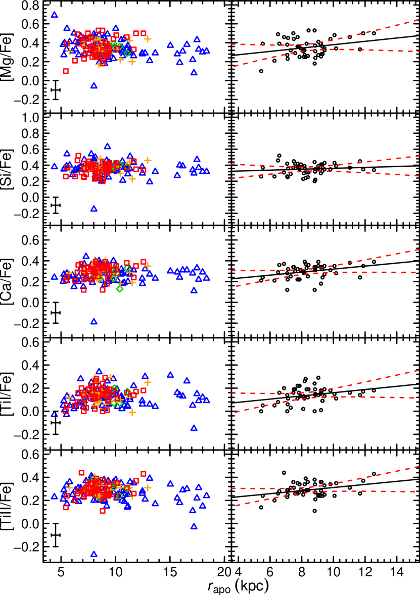
Figure 26.— Computed $\rm[\alpha/Fe]$ ratios vs. $r_{\rm apo}$ (column 4 of Table 4) for our sample of stars with $\rm[Fe/H]<-1.2$. Symbols and colors are the same as Figure 24. Recall that the left-hand side shows all populations, while the right-hand side shows only the stars assigned to the thick disk.

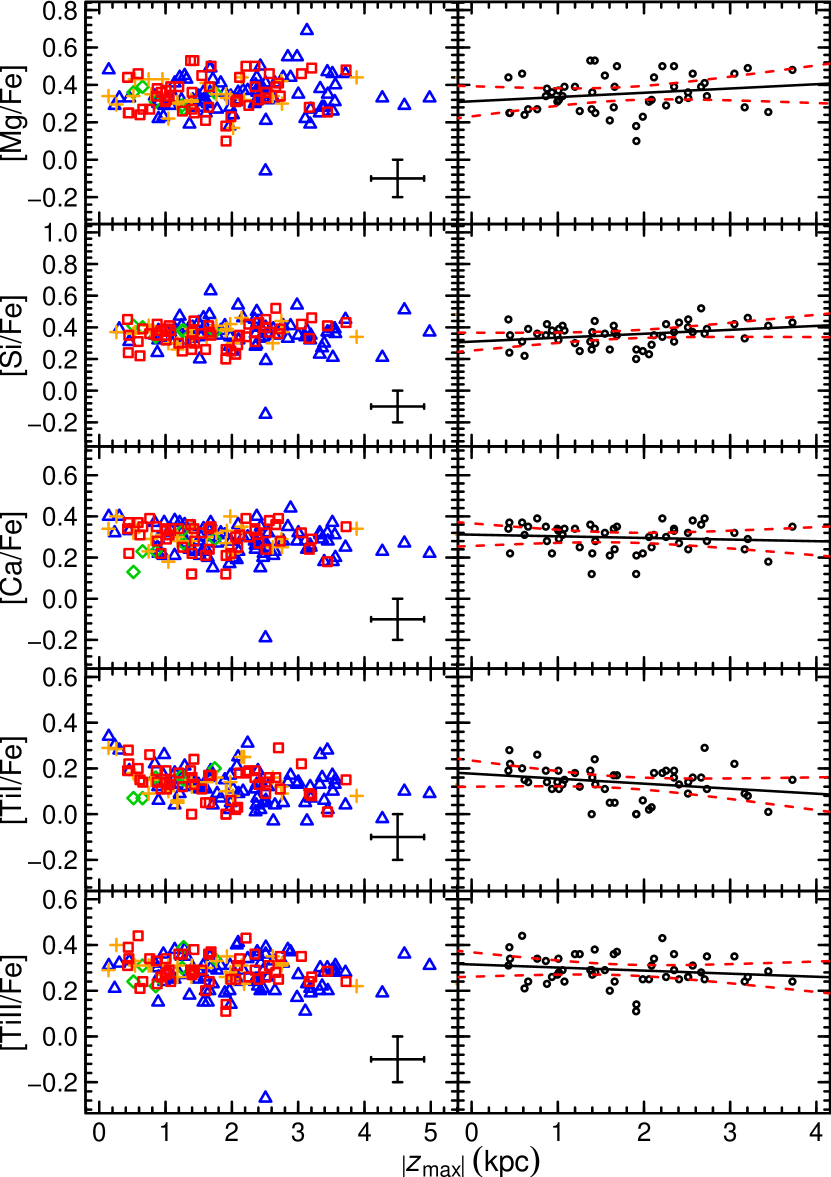
Figure 27.— Computed $\rm[\alpha/Fe]$ ratios vs. $|z_{\rm max}|$ (column 5 of Table 4) for our sample of stars with $\rm[Fe/H]<-1.2$. Symbols and colors are the same as Figure 24. Recall that the left-hand side shows all populations, while the right-hand side shows only the stars assigned to the thick disk.

7.3. High Angular Momentum Halo

In Figure 15, it is evident that some stars assigned to the thick disk have overlapping $V_{\Theta}$ velocities with the high-velocity tail of the halo. Further, we found that there is a second, low-metallicity peak in the metallicity distribution of the thick disk (Figure 17).

We investigated the possibility that the low metallicity peak might indicate contamination from the high-angular momentum halo by plotting $\rm[Fe/H]$ and each of the $\rm[\alpha/Fe]$ ratios versus $V_{\Theta}$, which are shown in Figure 28. Within the thick disk, there is no trend of $\rm[\alpha/Fe]$ or $\rm[Fe/H]$ with $V_{\Theta}$, except perhaps at the regime when the thick disk overlaps with the thin disk. This implies that there is no difference between those stars that might kinematically be a part of the tail of the halo and those that have azimuthal velocities that are too high to be halo. Thus, Figure 28 shows there is no difference between the halo and thick disk, as was found when comparing the $\rm[\alpha/Fe]$ ratios versus $\rm[Fe/H]$.

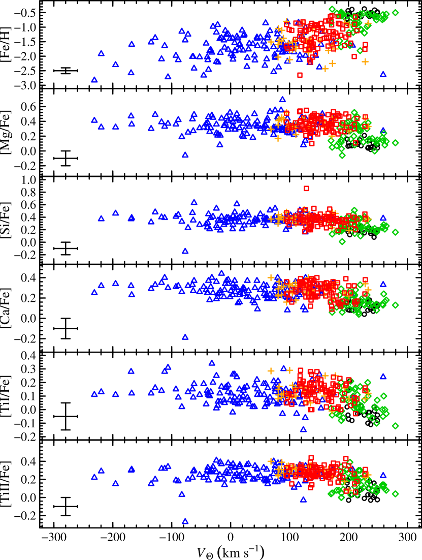
Figure 28.— $\rm[Fe/H]$ and $\rm[\alpha/Fe]$ ratios vs. $V_{\Theta}$ for our sample of stars. Symbols and colors are the same as Figure 23. Note that the error in $V_{\Theta}$ is typically lower than the error bar shown.

In Figure 29, we plot the velocity distributions for only stars with $\rm[Fe/H]<-1.2$. The thick disk distributions still show a clear distinction from the halo distributions. It is therefore reasonable to assume these stars could still be thick disk stars.

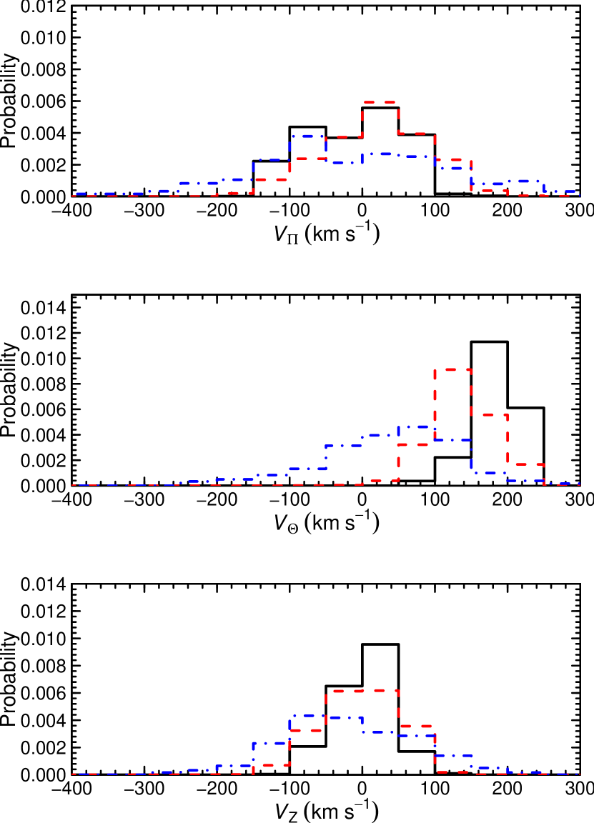
Figure 29.— Distribution of $V_{\Pi}$ (top panel), $V_{\Theta}$ (middle panel), and $V_{Z}$ (bottom panel) velocities for stars with $\rm[Fe/H]<-1.2$, given the PDF value that they belong to the thin disk (solid black), thick disk (dashed red), and halo (dot-dashed blue). Note that each distribution was created by summing the PDF values within a given velocity bin. The distributions were then normalized such that the total area equals unity.

7.4. A Lagged Thick Disk Component?

Some have proposed (e.g., Carollo et al., 2010) that the kinematics of the metal-poor thick disk may differ from the canonical thick disk. In this case the metal-poor component would have higher velocity dispersions and a slower rotational velocity. To investigate the effects of such a component on our results, we adopted a $\langle V_{\Theta}\rangle=-100$ ${\rm km~{}s^{-1}}$ and velocity dispersions of $(\sigma_{\Pi},\sigma_{\Theta},\sigma_{Z})=(63,70,60)$ ${\rm km~{}s^{-1}}$ for the lagged component (see Gilmore et al., 2002) in addition to the thin disk, canonical thick disk, and halo components. We then computed new population assignments for the stars. This increased the number of stars assigned to the thick disk population by 22 stars; 16 of which were formerly assigned to the thick/halo population, 4 formerly halo, and 2 formerly thin/thick.

The overall shape of the iron distribution did not change for the combined thick disk components. Further, the mean $\rm[\alpha/Fe]$ ratios showed no difference from that of the canonical thick disk alone, while the gradients in both $\rm[Fe/H]$ and $\rm[\alpha/Fe]$ changed by less than $0.01~{}{\rm dex~{}kpc}^{-1}$. Our results therefore do not show any significant change by including a lagged component for the thick disk.

8. IMF Variation

In R10, we established that our metal-poor thick-disk giants stars formed during a period of rapid star formation, primarily pre-enriched by core-collapse supernova (e.g. SNe II). In this section we quantify the level of IMF variation (specifically the slope, $x$, of the IMF) of the massive stars that ended as a core-collapse SNe using model yields and comparing with the scatter in our data.

For this test, we adopted the mass-dependent Mg and Fe yields of SNe II from Kobayashi et al. (2006). we can then compute the massive-star IMF-averaged yield for each element using different IMF slopes, $x$, by:

$$Y_{\rm IMF}=\int_{M_{\rm lo}}^{M_{\rm up}}Y(M)~{}M^{-(1+x)}~{}dM$$ (15)

where $Y(M)$ is the mass-dependent yield, $M_{\rm lo}=13$ ${\rm M}_{\odot}$, and $M_{\rm up}=40$ ${\rm M}_{\odot}$.

Figure 30 shows a plot of ${\rm[Mg/Fe]_{IMF}}$ versus the IMF slope, $x$. We used this plot to determine the spread in IMF slope values from the scatter in the [Mg/Fe] ratios of the stars assigned to the thick disk.

Figure 30.— IMF-averaged ${\rm[Mg/Fe]_{IMF}}$ vs. the IMF slope, $x$, computed using equation (15). Note that as $x$ decreases, the ratio of Mg-to-Fe increases, and that the relationship is nearly linear. The Salpeter IMF occurs for $x=2.35$.

From Figure 30, a small difference in IMF slope implies a large difference in $\rm[\alpha/Fe]$ (in this case ${\rm[Mg/Fe]_{IMF}}$), better than scatter. Previously, we showed that the thick disk has no scatter outside of random errors in all $\rm[\alpha/Fe]$ ratios. This leaves no room for any variation in the IMF. Further, this implies that the ISM was well-mixed prior to star formation. Similarly, the difference between the mean [Mg/Fe] values of the halo and thick disk is 0.03 dex, well within our 0.1 dex errors. This illustrates that the halo and metal-poor thick disk came from a very similar massive star IMF.

9. Orbital Eccentricity

Sales et al. (2009, hereafter S09) investigated the utility of orbital eccentricity ($\varepsilon$) distributions as a tool for distinguishing several scenarios for the formation of the thick disk. They compared the predictions from several simulations of the formation of thick disks and found that the $\varepsilon$-distributions also provide a robust diagnostic to distinguish between stellar populations that form in the simulated galaxy (in situ) versus those that are formed in a satellite galaxy and accreted into the simulated galaxy for all scenarios that involve both types of populations. The accreted population dominates high eccentricities, while the in situ population dominates the lower eccentricity bins. It is important to note that only one realization, with a specific set of initial conditions, for each formation scenario was used to compute the eccentricity distributions. This is, however, sufficient since there is no reason that the given simulations are not representative of that scenario.

It is important to note that we cannot use our population assignments when constructing the distribution of orbital eccentricities for the thick disk. The shape and extent of the tail of the thick-disk distribution is biased by our definition of ‘thick disk’ during our population analysis. We simulated our analysis by creating 1000 model stars in which their distance and Galactic coordinates were randomly chosen assuming a uniform distribution, and their 3-dimensional space motion was randomly selected using the ‘thick disk’ Gaussian definition in Table 5. Each model star was then run through our orbital program to determine the orbital eccentricity. Only 12% of these model thick disk stars had $\varepsilon>0.6$, which indicates that our definition of thick disk does not allow for many stars on highly eccentric orbits. Further, this could also affect the shape of the right side of the eccentricity distributions.

We therefore followed the procedure of S09 to investigate the orbital eccentricities of our metal-poor thick disk sample stars, calculated in §5.7 for the last orbit of a star. In this case, we computed the $\varepsilon$-distribution of stars with $V_{\Theta}>50$ ${\rm km~{}s^{-1}}$and $1\leq|z|/z_{\rm d}\leq 3$, where $z_{\rm d}=0.9$ kpc. This distribution is shown in Figure 31. To estimate the effects of distance errors on the distribution, we also plot the resultant eccentricity distribution when distances are increased and decreased by 20%.

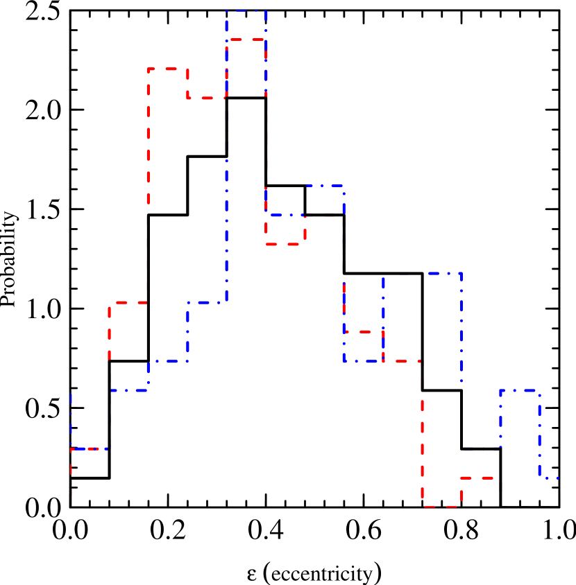
Figure 31.— The distribution of orbital eccentricities for those stars in our sample with $V_{\Theta}>50$ ${\rm km~{}s^{-1}}$and $1\leq|z|/z_{\rm d}\leq 3$, where $z_{\rm d}=0.9$ kpc. The distribution when the distances to the stars are decreased or increased by 20% are given by red, dashed and blue, dot-dashed lines, respectively.

The majority of the stars in this sample appear to exhibit low orbital eccentricities, with the distribution peaking around $\varepsilon\sim 0.3-0.4$. Our distribution does not show a strong resemblance to any of the distributions found in S09. The tail to high eccentricity somewhat resembles that of the direct accretion scenario of Abadi et al. (2003). The peak at lower eccentricities is significantly lower than predicted by the direct accretion scenario, and is more consistent with the predictions of models wherein the stars of the thick disk were primarily formed in situ. It is possible that we are under-sampling the low-eccentricity bins since we do not have many stars at the peak of the thick-disk metallicity distribution, $\rm[Fe/H]\sim-0.6$ . It is likely that including more metal-rich thick-disk stars could significantly change the distribution of eccentricities.

10. Discussion

In this work, we analyzed our full sample of metal-poor thick disk candidate stars. The MS/SG stars, added to our giant star sample from R10, were primarily assigned to the thin disk and thin/thick populations, and increased the number of stars with $\rm[Fe/H]>-0.8$. We found that our findings from R10 were unchanged, in that the $\rm[\alpha/Fe]$ ratios for the metal-poor thick-disk stars are enhanced and show low scatter ($<0.09$ dex, within the error of 0.1 dex), indicating that star formation took place on a short timescale in which the metal-poor thick disk was pre-enriched by core-collapse SNe from an invariant massive star IMF. Further, the metal-poor thick disk and halo were most likely pre-enriched by the same massive star IMF, showing a difference in $\alpha$-enhancement of $<0.03$ dex. The low amplitude of scatter in the element ratios indicates that the ISM from which the stars formed was well-mixed.

As discussed in R10, the enhancement and low scatter of $\rm[\alpha/Fe]$ in the thick disk are evidence that the formation of the thick disk had little influence by the late, direct accretion of stars from dwarf galaxies. The $\alpha$-enhancement in the metal-poor thick disk contrasts with the expectations from models that have direct accretion up until about $\sim 6$ Gyr ago (e.g., Abadi et al., 2003), assuming that the accreted dwarfs formed stars and self-enriched similarly to the surviving dwarfs. In this case, the stars accreted would then look chemically different from our metal-poor thick-disk stars (see R10). Further, the distribution of orbital eccentricities for our stars does not resemble that of the direct accretion scenario, instead resembling a population that was formed in situ.

Using the full RAVE catalog of stars, Wilson et al. (2011) also computed orbital eccentricities for a more uniform sample of thick disk stars, finding results consistent with ours. On the other hand, Dierickx et al. (2010) looked at the orbital eccentricities of a sample of thick-disk candidate stars selected from the Sloan Digital Sky Survey, and found that their distribution is inconsistent with the thick disk forming from radial migration only or heating due to mergers only. Casetti-Dinescu et al. (2011), however, show that their distribution, using data from RAVE and the Southern Proper Motion Program, is most consistent with the heating and merger scenarios. Overall, these results still support our finding that the stars in the thick disk primarily formed in situ. It is also important to note that our distribution of eccentricities is the first to have the metal-poor thick disk well-represented, but selection biases may be affecting the shape of the distribution.

From previous investigations of the local neighborhood and our more extended sample, it is clear that the thick disk is old, and had to form stars during a short, rapid burst to produce the $\alpha$-enhancement we detect. Direct accretion of stars from dwarf galaxies that formed a long time ago (about $10$ Gyr ago) during a period of rapid star formation is then still viable. These types of dwarf galaxies, however, are extremely rare. All known dwarf spheroidal galaxies typically have extended star formation and lower $\alpha$-enhancement at the same $\rm[Fe/H]$ range of the metal-poor thick disk (see review by Tolstoy et al., 2009). We can therefore conclude with confidence that the late accretion of stars from satellite galaxies did not play a role in the formation of the thick disk.

Models that include a significant component of the thick disk formed in situ, however, need to be further assessed. These models all imply or directly predict a thick disk with high $\alpha$-enhancement. Further, given the errors in the distances to our stars, and the effects of our definition of ‘thick disk’, the orbital eccentricity distribution of our sample of metal-poor thick disk stars does not show any direct inconsistencies with the distributions in S09 for these scenarios. It is interesting to note, however, that the S09 $\varepsilon$-distribution for the heating scenario shows a significant fraction of accreted stars that comprise the thick disk. Unless all of these accreted stars were assimilated into the thick disk at early times (as stated above), then this fraction of stars would have lower $\alpha$-enhancement than we see in our sample.

The models also show differences in their predictions for radial or vertical abundance variation. Observational evidence for abundance gradients in the thick disk are therefore very important. The majority of previous studies with high resolution analyses have shown no evidence for a vertical metallicity gradient in the thick disk (cf., Mishenina et al., 2004; Soubiran & Girard, 2005). These studies, however, primarily include nearby stars with $\rm[Fe/H]\geq-1.5$, while our gradient is computed for thick-disk stars with $\rm[Fe/H]<-1.2$. More recent studies have shown evidence for the possibility of a vertical metallicity gradient. Looking at stars at high Galactic latitudes and $z<4$ kpc, Siegel et al. (2009) found that iron abundance decreases with vertical height by $-0.15~{}{\rm dex~{}kpc^{-1}}$. This data, however, may have strong contamination from the thin disk. Ivezić et al. (2008) found a $0.1-0.2~{}{\rm dex~{}kpc^{-1}}$ metallicity gradient for stars selected from SDSS that lie a vertical heights, $z=1-2$ kpc. At these heights, the likelihood of contamination from thin disk is small, and so one could deduce that they were looking at mostly thick disk stars.

The stars in our sample assigned to the thick disk lie within about $\pm 2$ kpc radially about the Sun, and have vertical distances of $|z|<3$ kpc. Due to biases introduced by our analysis technique, we only investigated abundance gradients for those stars with $\rm[Fe/H]\leq-1.2$. We found very small amplitude radial and vertical gradients, $<0.03\pm 0.02~{}{\rm dex~{}kpc^{-1}}$, in the $\alpha$-enhancement of the metal-poor thick disk. This further verifies that the ISM was well mixed during star formation. Further, we found a small $+0.01\pm 0.04~{}{\rm dex~{}kpc^{-1}}$ radial iron abundance gradient, however, it is possible that $\rm[Fe/H]$ significantly changes by $\sim-0.09\pm 0.05~{}{\rm dex~{}kpc^{-1}}$ with vertical height above the Galactic plane. A fit resulting in no gradient is still possible, however, within 2-sigma confidence limits. Note that it is possible that including the more metal-rich thick disk would significantly change the amplitude of the slope of the gradients. Our results, however, resemble those found by groups studying the more metal-rich thick disk (as given above).

A vertical metallicity gradient is expected from the dissipational collapse model. Additionally, a thick disk with uniformly enhanced $\alpha$-abundances is also likely if the collapse took several millions of years, as predicted (Burkert et al., 1992). Rapid star formation early on during the heating scenario will produce enhanced $\rm[\alpha/Fe]$ ratios, while small amplitude radial abundance gradients are also possible. The merger model also predicts a high star formation rate from gas dissipation, and hence enhanced $\rm[\alpha/Fe]$ ratios, but the final thick disk is expected to have uniform abundance ratios. Although our data does not directly disagree with a uniform disk, a significant iron abundance gradient would challenge this scenario. It is also important to note that there is direct accretion of stars during the merger and heating scenarios, which can occur until late times. Late accretion of stars must therefore be extremely minimal for the abundances of the final thick disks in these scenarios to match the low scatter in $\rm[\alpha/Fe]$ for our thick disk stars.

An $\alpha$-enhanced thick disk is also implied from the clumpy disk model in which there is rapid star formation from internal processes with rapid mixing by strong turbulence. Additionally, the thick disk in the radial migration model has high $\rm[\alpha/Fe]$ ratios, since the stars in the inner disk undergo rapid star formation and then move outward, (see Schönrich & Binney, 2009b). No radial abundance gradients are predicted due to blurring across radii in the radial migration model and the turbulent mixing in the clumpy disk model. Note that the radial migration model does not include effects from the bar of the Galaxy. It is possible that the combination of the bar and spiral arms could result in a very efficient mixing mechanism, which could cause variation in the metallicity of the thick disk as a function of radius (Minchev & Famaey, 2010; Minchev et al., 2011). It is unclear, however, if a vertical iron abundance gradient is possible in either the radial migration model or clumpy disk model, indicating that more modeling must be done to ascertain this chemical signature.

11. Conclusions

The metal-poor thick disk of the Milky Way Galaxy is enhanced in the $\alpha$-elements and reaches to metallicities down to -2 dex. We find that the stars in the thick disk most likely formed within the potential well of the Milky Way Galaxy. Direct accretion of stars could have occurred at very early times ($\sim 1$ Gyr after the start of star formation) in the formation of the thick disk, but the later contribution of accreted stars into the thick disk was very minimal. The abundance trends of the metal-poor thick disk tends to favor models which result in a thick disk with a significant vertical metallicity gradient, however, a uniformly enhanced thick disk is still possible. Additionally, the radial migration and internal star formation at high redshift may have also contributed to the formation of the thick disk, but more work needs to be done to quantify the abundance trends for these scenarios.

References

- Abadi et al. (2003) Abadi, M. G., Navarro, J. F., Steinmetz, M. & Eke, V. R. 2003, ApJ, 597, 21
- Alves-Brito et al. (2010) Alves-Brito, A., Meléndez, J., Asplund, M., Ramírez, I., & Yong, D. 2010, A&A, 513, A35
- Aoki et al. (2005) Aoki, W., et al. 2005, ApJ, 632, 611
- Asplund et al. (1999) Asplund, M., Nordlund, Å., Trampedach, R., & Stein, R. F. 1999, A&A, 346, L17
- Bensby et al. (2003) Bensby, T., Feltzing, S. & Lundstrom, I. 2003, A&A, 410, 527
- Bergemann (2011) Bergemann, M. 2011, MNRAS, 357
- Bernstein et al. (2003) Bernstein, R., Shectman, S. A., Gunnels, S. M., Mochnacki, S. & Athey, A. E. 2003, SPIE, 4841, 1649
- Bonifacio et al. (2000) Bonifacio, P., Monai, S., & Beers, T. C. 2000, AJ, 120, 2065
- Bournaud et al. (2009) Bournaud, F., Elmegreen, B. G., & Martig, M. 2009, ApJ, 707, L1
- Breddels et al. (2010) Breddels, M. A., et al. 2010, A&A, 511, A90
- Brewer & Carney (2006) Brewer, M.-M. & Carney, B. W. 2006, AJ, 131, 431
- Brook et al. (2005) Brook, C. B., Gibson, B. K., Martel, H. & Kawata, D. 2005, ApJ, 630, 298
- Brook et al. (2004) Brook, C. B., Kawata, D., Gibson, B. K., & Freeman, K. C. 2004, ApJ, 612, 894
- Burkert et al. (1992) Burkert, A., Truran, J. W. & Hensler, G. 1992, ApJ, 391, 651
- Burnett & Binney (2010) Burnett, B., & Binney, J. 2010, MNRAS, 407, 339
- Carollo et al. (2010) Carollo, D., et al. 2010, ApJ, 712, 692
- Casetti-Dinescu et al. (2011) Casetti-Dinescu, D. I., Girard, T. M., Korchagin, V. I., & van Altena, W. F. 2011, ApJ, 728, 7
- Chiba & Beers (2000) Chiba, M. & Beers, T. C. 2000, AJ, 119, 2843
- Demarque et al. (2004) Demarque, P., Woo, J.-H., Kim, Y.-C. & Yi, S. K. 2004, ApJS, 155, 667
- Dierickx et al. (2010) Dierickx, M., Klement, R., Rix, H.-W., & Liu, C. 2010, ApJ, 725, L186
- Fulbright (2000, hereafter F00) Fulbright, J. P. 2000, AJ, 120, 1841 (F00)
- Fulbright (2002) Fulbright, J. P. 2002, AJ, 123, 404
- Gilmore & Reid (1983) Gilmore, G., & Reid, N. 1983, MNRAS, 202, 1025
- Gilmore & Wyse (1991) Gilmore, G., & Wyse, R. F. G. 1991, ApJ, 367, L55
- Gilmore et al. (2002) Gilmore, G., Wyse, R. F. G. & Norris, J. E. 2002, ApJ, 574, 39
- Girardi et al. (2002) Girardi, L., Bertelli, G., Bressan, A., Chiosi, C., Groenewegen, M. A. T., Marigo, P., Salasnich, B., & Weiss, A. 2002, A&A, 391, 195
- González Hernández & Bonifacio (2009) González Hernández, J. I., & Bonifacio, P. 2009, A&A, 497, 497
- Grevesse et al. (1996) Grevesse, N., Noels, A., & Sauval, A. J. 1996, Cosmic Abundances, 99, 117
- Hayashi & Chiba (2006) Hayashi, H., & Chiba, M. 2006, PASJ, 58, 835
- Hernquist (1990) Hernquist, L. 1990, ApJ, 356, 359
- Ivans et al. (2001) Ivans, I. I., Kraft, R. P., Sneden, C., Smith, G. H., Rich, R. M., & Shetrone, M. 2001, AJ, 122, 1438
- Ivezić et al. (2008) Ivezić, Ž., et al. 2008, ApJ, 684, 287
- Iwamoto et al. (1999) Iwamoto, K., Brachwitz, F., Nomoto, K., Kishimoto, N., Umeda, H., Hix, W. R., & Thielemann, F.-K. 1999, ApJS, 125, 439
- Jones & Wyse (1983) Jones, B. J. T., & Wyse, R. F. G. 1983, A&A, 120, 165
- Jurić et al. (2008) Jurić, M., et al. 2008, ApJ, 673, 864
- Kaufer et al. (1999) Kaufer, A., Stahl, O., Tubbesing, S., Nørregaard, P., Avila, G., Francois, P., Pasquini, L., & Pizzella, A. 1999, The Messenger, 95, 8
- Kazantzidis et al. (2008) Kazantzidis, S., Bullock, J. S., Zentner, A. R., Kravtsov, A. V., & Moustakas, L. A. 2008, ApJ, 688, 254
- Kobayashi et al. (2006) Kobayashi, C., Umeda, H., Nomoto, K., Tominaga, N., & Ohkubo, T. 2006, ApJ, 653, 1145
- Kraft & Ivans (2003) Kraft, R. P., & Ivans, I. I. 2003, PASP, 115, 143
- Kroupa (2002) Kroupa, P. 2002, Science, 295, 82
- Kurucz (1993) Kurucz, R. L. 1993, IAU Colloq. 138: Peculiar versus Normal Phenomena in A-type and Related Stars, 44, 87
- Majewski (1993) Majewski, S. R. 1993, ARA&A, 31, 575
- Marigo et al. (2008) Marigo, P., Girardi, L., Bressan, A., Groenewegen, M. A. T., Silva, L., & Granato, G. L. 2008, A&A, 482, 883
- Masana et al. (2006) Masana, E., Jordi, C., & Ribas, I. 2006, A&A, 450, 735
- Mashonkina et al. (2011) Mashonkina, L., Gehren, T., Shi, J.-R., Korn, A. J., & Grupp, F. 2011, A&A, 528, A87
- Matijevič et al. (2010) Matijevič, G., et al. 2010, AJ, 140, 184
- Matteucci (2003) Matteucci, F. 2003, Ap&SS, 284, 539
- Matteucci & Brocato (1990) Matteucci, F., & Brocato, E. 1990, ApJ, 365, 539
- McCall (2004) McCall, M. L. 2004, AJ, 128, 2144
- Minchev & Famaey (2010) Minchev, I., & Famaey, B. 2010, ApJ, 722, 112
- Minchev et al. (2011) Minchev, I., Famaey, B., Combes, F., Di Matteo, P., Mouhcine, M., & Wozniak, H. 2011, A&A, 527, A147
- Mishenina et al. (2004) Mishenina, T. V., Soubiran, C., Kovtyukh, V. V., & Korotin, S. A. 2004, A&A, 418, 551
- Miyamoto & Nagai (1975) Miyamoto, M., & Nagai, R. 1975, PASJ, 27, 533
- Nissen & Schuster (2010) Nissen, P. E., & Schuster, W. J. 2010, A&A, 511, L10
- Quinn et al. (1993) Quinn, P. J., Hernquist, L. & Fullagar, D. P. 1993, ApJ, 403, 74
- Pietrinferni et al. (2004) Pietrinferni, A., Cassisi, S., Salaris, M., & Castelli, F. 2004, ApJ, 612, 168
- Pont & Eyer (2004) Pont, F., & Eyer, L. 2004, MNRAS, 351, 487
- Reddy & Lambert (2008) Reddy, B. E., & Lambert, D. L. 2008, MNRAS, 391, 95
- Reddy et al. (2006) Reddy, B. E., Lambert, D. L. & Allende Prieto, C. 2006, MNRAS, 367, 1329
- Ruchti et al. (2010) Ruchti, G. R., et al. 2010, ApJ, 721, L92
- Salaris et al. (1993) Salaris, M., Chieffi, A., & Straniero, O. 1993, ApJ, 414, 580
- Sales et al. (2009) Sales, L. V., et al. 2009, MNRAS, 400, L61
- Salpeter (1955) Salpeter, E. E. 1955, ApJ, 121, 161
- Schlegel et al. (1998) Schlegel, D. J., Finkbeiner, D. P., & Davis, M. 1998, ApJ, 500, 525
- Schmidt (1959) Schmidt, M. 1959, ApJ, 129, 243
- Schönrich & Binney (2009a) Schönrich, R., & Binney, J. 2009a, MNRAS, 396, 203
- Schönrich & Binney (2009b) Schönrich, R., & Binney, J. 2009b, MNRAS, 399, 1145
- Sellwood & Binney (2002) Sellwood, J. A., & Binney, J. J. 2002, MNRAS, 336, 785
- Siegel et al. (2009) Siegel, M. H., Karataş, Y., & Reid, I. N. 2009, MNRAS, 395, 1569
- Smith et al. (2007) Smith, M. et al. 2007, MNRAS, 379, 755
- Sneden (1973) Sneden, C. 1973, ApJ, 184, 839
- Soubiran et al. (2003) Soubiran, C., Bienaymé, O. & Siebert, A. 2003, A&A, 398, 141
- Soubiran & Girard (2005) Soubiran, C., & Girard, P. 2005, A&A, 438, 139
- Sousa et al. (2007) Sousa, S. G., Santos, N. C., Israelian, G., Mayor, M. & Monteiro, M. J. P. F. G. 2007, A&A, 469, 783
- Steinmetz et al. (2006) Steinmetz, M. et al. 2006, AJ, 132, 1645
- Thévenin & Idiart (1999) Thévenin, F., & Idiart, T. P. 1999, ApJ, 521, 753
- Thorsett & Chakrabarty (1999) Thorsett, S. E., & Chakrabarty, D. 1999, ApJ, 512, 288
- Tinsley (1980) Tinsley, B. M. 1980, Fund. Cosmic Phys., 5, 287
- Tolstoy et al. (2009) Tolstoy, E., Hill, V., Tosi, M. 2009, ARA&A, 47, 371
- van Leeuwen (2007) van Leeuwen, F. 2007, A&A, 474, 653
- Velazquez & White (1999) Velazquez, H., & White, S. D. M. 1999, MNRAS, 304, 254
- Villalobos & Helmi (2008) Villalobos, Á., & Helmi, A. 2008, MNRAS, 391, 1806
- Walker & Diego (1985) Walker, D. D. & Diego, F. 1985, MNRAS, 217, 355
- Wang et al. (2003) Wang, S.-i., et al. 2003, Proc. SPIE, 4841, 1145
- Weidemann (2000) Weidemann, V. 2000, A&A, 363, 647
- Wilson et al. (2011) Wilson, M. L., et al. 2011, MNRAS, 260
- Woosley & Heger (2007) Woosley, S. E., & Heger, A. 2007, Phys. Rep., 442, 269
- Yi et al. (2001) Yi, S., Demarque, P., Kim, Y.-C., Lee, Y.-W., Ree, C. H., Lejeune, T. & Barnes, S. 2001, ApJS, 136, 417
- Zwitter et al. (2008) Zwitter, T., et al. 2008, AJ, 136, 421
- Zwitter et al. (2010) Zwitter, T., et al. 2010, A&A, 522, A54