Two-photon driven nonlinear dynamics and entanglement of an atom in a non uniform cavity

Abstract

In this paper we study the dynamics in the general case for a Tavis Cummings atom in a non-uniform cavity. In addition to the dynamical Stark shift, the center-of-mass motion of the atom and the recoil effect are considered in both - the weak and the strong cavity atom coupling regimes. It is shown that the spatial motion of the atom inside the cavity in the resonant case leads to a transition between topologically different solutions. This effect is manifested by a singularity in the inter-level transition spectrum. In the non-resonant case, the spatial motion of the atom leads to a switching of the spin orientation. In both effects, the key factor is the relation between the values of the Stark shift and the cavity field coupling constant. We also investigate the entanglement of an atom in the cavity with the radiation field. It is shown that the entanglement between the atom and the field, usually quantified in terms of purity, decreases with increasing the Stark shift.

I Introduction

Cavity quantum electrodynamics (CQED) is an active field of research focusing on the quantum nature of the interaction of atoms with photons in high-finesse cavities Aoki ; Mabuchi ; Hood ; Raimond . Current issues of interest includes entanglement and quantum correlations Shevchenko ; Maruyama ; Buluta ; Amico ; Mintert . The standard model of CQED is a two level system in a quantum cavity. This case has served as an example for the realization of quantum programming protocols and for quantum teleportation Bruss . A controlled system of several atoms is also promising as a candidate for multiqubit entangled state. In the simplest situation of a single atom interacting with few photons in the regime of strong coupling, the coherent atom-photon interaction overwhelms incoherent dissipative processes.The system can then be described by the Jaynes Cummings (JC) model Jaynes ; Schleich which captures the interaction of a single cavity mode with a frequency resonant with the transition frequency of the two lowest energy levels of the atom. The interactions between the atom and the radiation field should, however, involve not only the internal atomic transitions and field states but also should account for the center-of-mass motion of the atom and for recoil effects. Since the motion of the atom in a cavity and inter-level transitions are connected to each other, the dynamics in a non-uniform cavity becomes rather complicated. For particular values of parameters, the corresponding classical system manifests regular or chaotic behavior: Different types of motion are found, including Lévy flights and chaotic walking of an atom in a cavity Prants . Consequences of the non-uniform cavity are also decoherence effects, a decay of entanglement and of the teleportation fidelity Chotorlishvili .
The main goal of the present work is the study of the dynamics of $su(1,1)$ Tavis-Cummings (TC) system in a non-uniform cavity including the dynamical Stark shift (DSS) Joshi ; Rybin . This model describes two-photon transitions between the ground and the excited state via an intermediate state. The intermediate state can be eliminated from the equations of motion on the cost of introducing a dynamical Stark shift Joshi . In particular, we study the impact of DSS on the dynamics of TC atom in non-uniform cavities. We identify different types of dynamics and possible mechanisms of switching between them. In the first part we use a semiclassical approach, which is a natural approximation for large mean photon numbers in the cavity. We investigate the problem in both the strong and the weak atom-cavity coupling regimes. In the second part we go beyond the semiclassical approximation and evaluate the influence of the cavity being non-uniform and also of DSS on the degree of entanglement between the atom and the radiation field.

II Model

The Hamiltonian of a single TC atom placed in an ideal cavity reads:

$$\hat{H}=\frac{\hat{P}^{2}}{2m}+\big{(}\omega_{0}+\zeta\hat{a}^{+}\hat{a}\big{)}\hat{s}^{z}+\omega_{f}\hat{a}^{+}\hat{a}+g(x)\big{(}\hat{s}^{+}\hat{a}^{2}+\hat{s}^{-}(\hat{a}^{+})^{2}\big{)}.$$ (1)

Here $g(x)$ is the coupling constant between the atom and the radiation field, $\hat{a}$, $\hat{a}^{+}$ are the photon annihilation and creation operators, $\zeta$ is the strength of the Stark shift, leading to the intensity-dependent transition frequency. The atomic two-level systems are described by the spin operators $\hat{s}^{z}=\frac{1}{2}\sigma^{z}$, $\hat{s}^{\pm}=\frac{1}{2}\big{(}\sigma^{x}\pm i\sigma^{y}\big{)}$, where $\sigma_{x,y,z}$ are Pauli operators. If the initial kinetic energy of the system is small $\frac{P^{2}}{2m}\ll d\sqrt{\frac{\hbar\omega_{0}n}{2\varepsilon_{0}V}}$, one can neglect the atomic motion and consider the standard TC model for uniform cavity $g(x)\approx\Omega_{0}$. Here $d$ is the atomic dipole moment, $V$ is the volume of the cavity, $\varepsilon_{0}$ is the electric constant and $n$ is the number of photons in the cavity. In the opposite limit the coupling constant $g(x)$ depends on the position of the atom inside the cavity. Therefore, the motion of the atom has a strong impact on the inter level transitions leading to a complex nonlinear dynamics. We show below that this nonlinearity and the complexity can be utilized for a spin orientation control. We assume a standard form for the dependence $g(x)=\Omega_{0}\cos k_{f}x$, where $k_{f}$ is the wave number in a lossless cavity of the Fabry-Perot type Prants . Consequently, the operator of the coordinate $\hat{x}$ together with the field and the spin operators form a complete set of observables. In what follows we will derive the Heisenberg equations for each observable and investigate the model (1) in the semi-classical approximation. We recall the standard commutation relations $\big{[}\hat{s}^{+};\hat{s}^{-}\big{]}=2\hat{s}^{z}$, $\big{[}\hat{s}^{z};\hat{s}^{\pm}\big{]}=\pm\hat{s}^{\pm}$, $\big{[}\hat{a};\hat{a}^{+}\big{]}=1$ and the expressions for the operators in the interaction representation $\hat{a}(t)=\hat{a}e^{-i\omega_{f}t}$, $\hat{a}^{+}(t)=\hat{a}^{+}e^{i\omega_{f}t}$. From the Heisenberg equations of motion $\frac{d\hat{A}}{dt}=\frac{\partial\hat{A}}{\partial t}+i\big{[}\hat{H};\hat{A}\big{]}$ and eq. (1) we infer

$$\frac{dx}{d\tau} = \alpha p,$$

$$\frac{dp}{d\tau} = -\sin x\cdot u,$$

$$\frac{du}{d\tau} = -\big{(}\delta+\frac{\Delta}{2}+\Delta s_{z}\big{)}v,$$ (2)

$$\frac{dv}{d\tau} = \big{(}\delta+\frac{\Delta}{2}+\Delta s_{z}\big{)}u+16\cos x\cdot s_{z}\cdot(N-s^{2}+2s_{z}^{2}),$$

$$\frac{ds_{z}}{d\tau} = -\cos x\cdot v.$$

Here the semi-classical averaging procedure is used Prants $x=k_{f}\langle\hat{x}\rangle$, $a_{y}=\langle\hat{a}_{y}\rangle$,$a_{x}=\langle\hat{a}_{x}\rangle$,$s_{x}=\langle\hat{s}_{x}\rangle$, $s_{y}=\langle\hat{s}_{y}\rangle$, $s_{z}=\langle\hat{s}_{z}\rangle$, $p=\frac{\langle\hat{P}\rangle}{k_{f}}$ and the following notations are introduced $\alpha=\frac{k^{2}_{f}}{m\Omega_{0}}$, $\delta=\frac{\omega_{f}-\omega_{0}}{\Omega_{0}}$, $\frac{\zeta}{\Omega_{0}}=\Delta$, $\tau=\Omega_{0}t$, $u=4(a_{x}s_{x}+a_{y}s_{y})$, $v=4(a_{x}s_{y}-a_{y}s_{x})$, $a^{2}_{x}+a^{2}_{y}-s^{2}_{z}=N=const$, $s_{x}^{2}+s_{y}^{2}+s_{z}^{2}=const$. We are interested in studying the system described by eq. (II) in different asymptotic limits. In particular, we focus on the dynamically induced control of the spin orientation and on switching. Our theoretical model can be realized easily in the experiment, e.g. by using Rydberg atoms and superconductive high-finesse cavities. For instance one may consider two-photon transitions between ${44}S_{1/2}\longleftrightarrow{43}S_{1/2}$ for rubidium atoms ${85}Rb$, or ${40}S_{1/2}\longleftrightarrow{39}S_{1/2}$ for cesium ${85}$ $Cs$. Such transitions proceed through the intermediate level $39P_{3/2}$ or $43P_{3/2}$, and are of the type -two photons allowed and one photon forbidden- Metwally . Depending on the principle quantum number $n$ the dynamical Stark shift is in the range $0<\zeta<100MHz$ Metwally . The cavity-atom coupling constant (which defines the time scale of our problem) is $\Omega_{0}\sim 1-10MHz$. Therefore, both limits $\Omega_{0}>\zeta$ and $\Omega_{0}<\zeta$ which will be discussed below are realistic from the experimental point of view.

III Adiabatic solutions: The Resonant case

In the semi-classical limit $N\gg s^{2}$ and within the regime of strong coupling $\alpha\ll 1$ eqs. (II) tend to the form

$$\frac{dx}{d\tau} = \alpha p,$$

$$\frac{dp}{d\tau} = -\sin x\cdot u,$$

$$\frac{du}{d\tau} = -\big{(}g+\Delta s_{z}\big{)}v,$$ (3)

$$\frac{dv}{d\tau} = \big{(}g+\Delta s_{z}\big{)}u+16\cos x\cdot s_{z}\cdot N,$$

$$\frac{ds_{z}}{d\tau} = -\cos x\cdot v.$$

From these relations it follows that the quantities

$$W=\frac{\alpha p^{2}}{2}-u\cos x+\frac{1}{2\Delta}(g+\Delta s_{z})^{2},\;\mbox{and}$$ (4)

$$u^{2}+v^{2}+16Ns^{2}_{z}=R^{2},~{}~{}~{}~{}~{}~{}~{}~{}~{}~{}~{}~{}~{}~{}~{}~{}~{}~{}$$

are integrals of motion. Here $g=\delta+\frac{\Delta}{2}$ is the de-tuning parameter.

The set of equations (III) is characterized by two time scales. The small parameter $\alpha\ll 1$ sets the time scale of the slow center-of-mass motion of the atom; the fast time scale is determined by the inter-level transitions. The separation of time scales allows us to split the set of equations of motion into two parts

$$\frac{d^{2}x}{d\tau^{2}}+\alpha u(\tau)\sin x=0.$$ (5)

and

$$\left\{\begin{array}[]{ll}\frac{du}{d\tau}=-(g+\Delta s_{z})v,\\ \frac{dv}{d\tau}=(g+\Delta s_{z})u+16cNs_{z},\\ \frac{ds_{z}}{d\tau}=-cv.\end{array}\right.$$ (6)

Due to the different time scales the slow parameter $c=\cos x$ in eq.(6) hardly varies on a reasonable time scales. Since $\dot{x}\sim\alpha,$ a small change of the variable $x(\tau)$ during the time interval $\tau<1/\alpha$ can be neglected. The period of the inter-level transitions (see Eq.(12) below) is, however, shorter than $T\ll 1/\alpha$. Consequently, the system performs a large number of inter-level transitions with $c=\cos(x(\tau))\sim const$. Utilizing the integrals of motion (4), one can derive a self-consistent equation for the spin operator $s_{z}(t)$:

$$\frac{ds_{z}}{d\tau}=-cv=-c\sqrt{R_{0}^{2}-\bigg{[}\frac{1}{2\Delta c}(g+\Delta s_{z})^{2}-\frac{W}{c}\bigg{]}^{2}-16Ns_{z}^{2}}.$$ (7)

Here in the energy of the system (4) we neglect the adiabatic part $\frac{\alpha p^{2}}{2}-u\cos(x)$. Consequently in the resonant case, i.e. for $g=0$ we have: $W=\frac{\triangle}{2},~{}~{}~{}$ $\omega_{0}=\omega_{f}+\frac{\zeta}{2}$, and eq. (7) can be rewritten in the form

$$\dot{s}_{z} = -cR_{0}\sqrt{(1-s_{z}^{2})(1-\kappa^{2}(1-s_{z}^{2}))},$$

$$\kappa = \frac{\Delta}{2cR_{0}},~{}~{}~{}R_{0}=4\sqrt{N}.$$ (8)

Consequently, the spin dynamics is described by the following solution

$$s_{z}(\tau)=\left\{\begin{array}[]{l}cn(cR_{0}\tau,\kappa),~{}~{}~{}~{}\kappa<1,\\ dn(cR_{0}\tau\kappa,\frac{1}{\kappa}),~{}~{}~{}~{}\kappa>1.\end{array}\right.$$ (9)

Here, $cn(cR_{0}\tau,\kappa)$ and $dn(cR\tau\kappa,\frac{1}{\kappa})$ are periodic Jacobi elliptic functions Abramowitz . For the other variables in eq. (6) we obtain (upon straightforward but laborious calculations) the expression

$$u(\tau)=-\frac{\Delta}{2c}\left\{\begin{array}[]{l}sn^{2}(cR_{0}\tau,\kappa),~{}~{}~{}~{}\kappa<1,\\ \frac{1}{\kappa^{2}}sn^{2}(cR_{0}\tau\kappa,\frac{1}{\kappa}),~{}~{}~{}~{}\kappa>1,\end{array}\right.$$ (10)

$$v(\tau)=\left\{\begin{array}[]{l}R_{0}sn(cR_{0}\tau;\kappa)dn(cR_{0}\tau;\kappa)~{}~{}~{}~{}~{}\kappa<1,\\ \frac{R_{0}}{\kappa}sn(cR_{0}\tau\kappa,\frac{1}{\kappa})\sqrt{1-\kappa^{2}sn^{2}(cR_{0}\tau\kappa,\frac{1}{\kappa})}~{}~{}~{}~{}\kappa>1.\end{array}\right.$$ (11)

From eq. (9) we conclude that, depending on the parameters of the problem, the dynamics of the level populations follow different solutions. These solutions are separated by the special value $\kappa=1$ of the bifurcation parameter $\kappa$ that signals the presence of topologically distinct solutions. In equation (9) the Jacobi elliptic functions are periodic in the argument with the period

$$T=\left\{\begin{array}[]{l}\frac{4}{cR_{0}}K(\kappa),~{}~{}~{}~{}~{}\kappa<1,\\ \frac{2}{cR_{0}\kappa}K(\frac{1}{\kappa}),~{}~{}~{}~{}\kappa>1,\end{array}\right.$$ (12)

where $K(\kappa)$ is the complete elliptic integral of the first kind Abramowitz . If $\kappa\rightarrow 1$, the period becomes infinite because $K(\kappa)\rightarrow\ln(4/\sqrt{1-\kappa^{2}})$. The evolution in this special case is given by the non-oscillatory soliton solutions:

$$s_{z}(\tau) = \frac{1}{\cosh(cR_{0}\tau)},$$

$$v(\tau) = R_{0}\frac{\sinh^{2}(cR_{0}\tau)}{\cosh^{2}(cR_{0}\tau)},$$ (13)

$$u(\tau) = -\frac{\Delta}{2c}\tanh^{2}(cR_{0}\tau).$$

The existence of a bifurcation parameter indicates that the solutions separated by it, have different topological properties. The phase trajectories corresponding to the solution $dn(cR_{0}\tau\kappa,\frac{1}{\kappa})$ are open and they describe a rotational motion, while trajectories corresponding to $cn(cR_{0}\tau,\kappa)$ are closed and they describe the oscillatory motion Zaslavsky . Due to the three independent variables in eq. (6) and the two integrals of motion (4), the system, described by eq. (6), is effectively one dimensional. Consequently, utilizing the integral of motion $R^{2}=R_{0}^{2}=16N$, $u(0)=0,~{}~{}v(0)=1,~{}~{}s_{z}(0)=1$ one can easily reduce the system (eqs. (6)) to the effective one dimensional model

$$H_{eff}=\frac{cv^{2}}{2}+\frac{\Delta^{2}}{8c}(1-s_{z}^{2})^{2}+\frac{c}{2}R_{0}^{2}s_{z}^{2}.$$ (14)

It is straightforward to conclude that the solutions eqs.(9)-(11) satisfy Hamilton’s equations for taking the canonical pair of variables as $(s_{z},v)$

$$\dot{s}_{z}=-H_{v}=-\frac{\partial H_{eff}}{\partial v},~{}~{}~{}~{}~{}~{}\dot{v}=H_{s_{z}}=\frac{\partial H_{eff}}{\partial s_{z}}.$$ (15)

Due to the nonlinearity, the model expressed by eq. (14) shows a rich topological structure of phase-space trajectories. Topologically different types of phase trajectories are divided by bifurcation points which can be identified by evaluating the following Poincare index Butenin

$$J=\frac{1}{2\pi}\oint d\big{\{}\tan^{-1}\big{[}-\frac{H_{s_{z}}}{H_{v}}\big{]}\big{\}}.$$ (16)

Here $\gamma$ is a contour around the equilibrium point $\dot{s}_{z}=0,\dot{v}=0$. From eqs. (14), and (16) we conclude for eq. (16) in the linear approximation

$$J\approx\frac{\cos^{2}(x)-\bigg{(}\frac{\zeta}{\Omega_{0}R_{0}}\bigg{)}^{2}}{\bigg{|}\cos^{2}(x)-\bigg{(}\frac{\zeta}{\Omega_{0}R_{0}}\bigg{)}^{2}\bigg{|}}.$$ (17)

The change of sign in $J$ from $J=1$ to $J=-1$ marks the transition from the stable equilibrium point to the unstable equilibrium saddle point, i.e. from closed to open phase trajectories. The bifurcation point is defined by the simple relation $x\sim\arccos\bigg{(}\frac{\zeta}{R_{0}\Omega_{0}}\bigg{)}$. Obviously, the key issue is the relation between the position $x(t)$ of the atom inside the cavity and the value of the dynamical shift of the frequency $\zeta$. For the determination of the transition time on a quantitative level we need the exact solution of Eq. (5). For further analysis of eqs. (5), and (6) we note that both solutions, given by eq. (9), contain the slow parameter $\kappa(\tau)=\big{(}\frac{\zeta}{2R_{0}\Omega_{0}\cos(x(\tau))}\big{)}^{1/2}$. If initially $\frac{\zeta}{2R_{0}\Omega_{0}}<1$, $\cos(x(0))\approx 1$, and $\kappa(0)<1$, even in this case, due to the adiabatic motion of the atom inside the cavity, the condition $\kappa(\tau)>1$ can be realized as well. This means that the motion of the atom inside a non-uniform cavity leads to a tunneling of the system, formally through the presence of a separatrix. This leads to a qualitative change of the dynamics of $s_{z}(\tau)$, i.e. eq. (9). The explicit solution for $x(t)$ can be found from eq. (5). Taking eq. (10) into account and considering $c=\cos x$ as an adiabatic parameter on the time scale $\tau\sim 1/R_{0}$ from eq. (5) we infer

$$\frac{d^{2}x}{d\tau^{2}}+f(x)=f(x)\cos(2R_{0}\tau).$$ (18)

Here $\varepsilon=\alpha\frac{\zeta}{\Omega_{0}}$, $f(x)=-\varepsilon\tan x$ is the small parameter that controls the time scale for the slow motion of the atom inside the cavity and which is definitely larger than the time of the inter-level transitions $\sqrt{\frac{2\Omega_{0}}{\alpha\zeta}}>\frac{1}{R_{0}}$ (since $N>1$, $\alpha<<1$). This means that during a slight change of the center of mass position from its initial value $x(\tau=0)=0$, the system performs multiple inter level transitions described by the first solution of given by eqs. (10).
For solving eqs. (18) we make use of the existence of a slow and a fast time scale and look for a solution of the form

$$x(\tau)=x_{1}(\tau)+\mu x_{2}(\tau).$$ (19)

The time scale for the slow variable $x_{1}(\tau)$ is governed by $1/\sqrt{\varepsilon}$. For the fast variable $x_{2}(\tau)$ we have $2R_{0}$, $2R_{0}\gg\sqrt{\varepsilon}$ and $\mu=\frac{\sqrt{\varepsilon}}{2R_{0}}$. With $f(x_{1}+\mu x_{2})\approx f(x_{1})+\mu x_{2}\big{(}\frac{\partial f}{\partial x}\big{)}_{x_{1}}$ we infer from eq. (19) that

$$\ddot{x}_{1}+\mu\ddot{x}_{2}=-f(x_{1})-\mu x_{2}\bigg{(}\frac{\partial f}{\partial x}\bigg{)}_{x_{1}}+\bigg{[}f(x_{1})+\mu x_{2}\bigg{(}\frac{\partial f}{\partial x}\bigg{)}_{x_{1}}\bigg{]}\cos(2R_{0}\tau).$$ (20)

After averaging over the time interval $1/2R_{0}$ we find

$$\ddot{x}_{1}\approx-f(x_{1})+\bigg{\langle}\mu x_{2}\bigg{(}\frac{\partial f}{\partial x}\bigg{)}_{x_{1}}\cos(2R_{0}\tau)\bigg{\rangle},$$ (21)

$$\mu x_{2}\approx-\mu x_{2}+f(x_{1})\cos(2R_{0}\tau).$$ (22)

Considering that $\mu\ddot{x}_{2}\sim\mu(2R_{0})^{2}x_{2}\sim 2R_{0}\sqrt{\varepsilon}x_{2}>\mu x_{2}\bigg{(}\frac{\partial f}{\partial x}\bigg{)}_{x_{1}}$ eq. (22). The result is

$$x_{2}(\tau) = -\bigg{[}\frac{f(x_{1})}{2R_{0}\sqrt{\varepsilon}}\bigg{]}\cos(2R_{0}\tau),$$

$$\ddot{x}_{1}(\tau) + f(x_{1})+\frac{1}{2}\frac{f(x_{1})}{4R_{0}^{2}}\bigg{(}\frac{\partial f}{\partial x}\bigg{)}_{x_{1}}=0.$$ (23)

Finally, in the linear approximation $f(x)=-\varepsilon x$ we conclude from eq. (III) that

$$x(\tau)=\sinh\bigg{(}\sqrt{\bigg{(}\frac{\zeta}{\alpha\Omega_{0}}-\frac{\zeta^{2}}{8R_{0}^{2}\Omega_{0}^{2}}\bigg{)}}\alpha\tau\bigg{)}\bigg{(}1+\frac{\alpha\zeta}{4R_{0}^{2}\Omega_{0}}\cos(2R_{0}\tau)\bigg{)}.$$ (24)

Using eqs. (III), and (24) we identify the time of bifurcation via

$$\tau_{b}\approx\sqrt{\frac{\Omega_{0}}{\alpha\zeta}}\ln\bigg{(}\arccos\big{(}\frac{1}{2R_{0}}\frac{\zeta}{\Omega_{0}}\big{)}\bigg{)},~{}~{}~{}k(\tau_{B})\sim 1.$$ (25)

Eq. (25) connects the values of the DSS parameter $\zeta$ and the birfurcation time $\tau$. This means that by observing the singularity in the spectrum of the Rabi oscillations of the inter-level transitions one can measure the frequency shift indirectly. Before proceeding with the non resonant case we summarize briefly the main results obtained for resonant case. The time scale of the spatial motion is described by the parameter $\alpha=\frac{k_{f}^{2}}{m\Omega_{0}}$. Since $\dot{x}\sim\alpha$ in the limit of a strong coupling between the atom and the cavity $\Omega_{0}>>\frac{k_{f}^{2}}{m}$, the motion of the atom inside of the cavity is adiabatic. Therefore, the system performs a large number of inter-level transitions before the slow adiabatic coordinate changes significantly. If the resonant condition $\zeta=2(\omega_{0}-\omega_{f})$ it met the inter-level transitions are described by topologically different solutions (cf. eq.(9)). The bifurcation parameter $k(x(\tau))$ depends on the center-of-mass coordinate of the atom $x(\tau)$ (eqs.(24), (25)). We argue that the existence of topologically different solutions divided by a bifurcation point is the reason why the spatial motion of the atom leads to singularities in the spectrum of inter-level transitions.

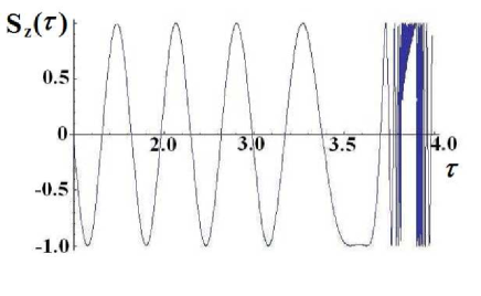
Figure 1: Color online. The time evolution of the atomic inversion, as descirbed by Eqs.(9, 24) for the following the parameters: $R_{0}=20$, $\alpha=5\cdot 10^{-3}$, $\zeta/\Omega_{0}=2$. When the parameter $\kappa(\tau)$ reaches the bifurcation values $\kappa(\tau_{b})=\bigg{(}\frac{\zeta}{2R_{0}\Omega_{0}\cos\big{(}x(\tau_{b})\big{)}}\bigg{)}^{1/2}\sim 1$, $\tau_{b}\approx\sqrt{\frac{\Omega_{0}}{\alpha\zeta}}\ln\bigg{(}\arccos\big{(}\frac{1}{2R_{0}}\frac{\zeta}{\Omega_{0}}\big{)}\bigg{)}\sim 4$ the inversion oscillations manifest a singularity.

IV Adiabatic solutions. Non resonant case

In the non-resonant case $g=\frac{1}{\Omega_{0}}\bigg{(}\frac{\zeta}{2}+\omega_{f}-\omega_{0}\bigg{)}\neq 0$, the solution of the equation (7) has the form

$$s_{z}(\tau)=1-\frac{1}{2W(cR\tau;g_{2};g_{3})-A_{2}}.$$ (26)

Here $W(cR\tau;g_{2};g_{3})$ is the Weierstrass function Abramowitz and the following notations are used:

$$g_{2} = 3A_{2}^{2}-2A_{1},~{}~{}~{}~{}~{}g_{3}=A_{1}A_{2}-A_{2}^{3}-\frac{1}{2}A_{0},$$

$$A_{2} = -\frac{1}{6}\bigg{(}1+\kappa^{2}\bigg{(}2+\frac{2g\Omega_{0}}{\zeta}\bigg{)}^{2}\bigg{)},~{}~{}~{}~{}~{}A_{1}=\frac{\kappa^{2}}{2}\bigg{(}2+\frac{2g\Omega_{0}}{\zeta}\bigg{)},$$ (27)

$$A_{0} = -\kappa^{2},~{}~{}~{}~{}\kappa=\frac{\zeta}{2\Omega_{0}R_{0}\cos(x)}.$$

For $\kappa<<1$ i.e. $\zeta<<2\Omega_{0}R_{0}$, $|A_{2}|\gg|A_{1}|$, $|A_{2}|\gg|A_{0}|$, $g_{2}=3A_{2}^{2}$ $g_{3}=-A_{2}^{3}$ and the roots of the equation

$$4x^{3}-g_{2}x-g_{3}=0,$$ (28)

satisfy the condition $e_{1}=-A_{2}$, $e_{2}=e_{3}=\frac{A_{2}}{2}$, $A_{2}=\frac{1}{6}\bigg{(}1+\frac{g}{R_{0}c}\bigg{)}^{2}$. Therefore we can use the following representation of the Weierstrass function Abramowitz :

$$W(\tau,g_{2},g_{3})=e_{1}+\frac{3}{2}e_{1}\cot^{2}\bigg{(}\sqrt{\frac{3}{2}e_{1}}\tau\bigg{)}.$$ (29)

As a result finally from eq. (26) we obtain

$$s_{z}(\tau)=1-\frac{1}{3e_{1}+\frac{3}{2}e_{1}\cot^{2}\bigg{(}\sqrt{\frac{3}{2}e_{1}}cR\tau\bigg{)}}.$$ (30)

From this expression we see that the motion of the atom leads to a switching of the spin orientation between the values $s_{z}(\tau)=1$ and $s_{z}(\tau)=1-\frac{1}{3e_{1}}$. The time interval for the switching is set by the simple relation $T=\frac{\pi}{2cR_{0}\sqrt{6e_{1}}}$. An illustration of this switching is shown by the simulations presented in Fig.2.

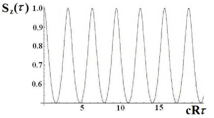
Figure 2: Switching of the spin projection $s_{z}(\tau)$ as induced by the motion of the atom inside the cavity. We have chosen $\frac{g}{R_{0}c}\sim 1$.

This dynamically induced switching can be utilized for the manipulation of the spin orientation. A further important issue is the principle difference between the results obtained for the non-resonant case ($\zeta\neq\omega_{f}-\omega_{0}$) from those results corresponding to the resonant case ($\zeta=2(\omega_{f}-\omega_{0})$). In contrast to the resonant case, for the non-resonant situation the spatial motion of the atom leads to a switching of the spin orientation. However, due to the absence of a bifurcation and topologically different solutions, the singularities in the spectrum of inter-level transition are absent.

V Dynamics for small DSS and minimal chaos

If the detuning between the radiation field and the spin splitting is larger than DDS, i.e. for $\delta=\frac{\omega_{f}-\omega_{0}}{\Omega_{0}}\gg\frac{\zeta}{\Omega_{0}}$, the equations of motion reduce to

$$1)\frac{d^{2}x}{d\tau^{2}}+\alpha u(\tau)\sin x=0,$$ (31)

$$2)\left\{\begin{array}[]{ll}\frac{du}{d\tau}=-\delta v,\\ \frac{dv}{d\tau}=\delta u+16cNs_{z},\\ \frac{ds_{z}}{d\tau}=-\cos xv.\end{array}\right.$$ (32)

Since $\alpha\ll 1,$ the adiabatic approximation is still valid and the eqs. (32) is analytically integrable. Introducing $u(\tau)=X(\tau)$, $v(\tau)=Y(\tau)$, $Z(\tau)=R_{0}s_{z}$, $C_{0}=-R_{0}\cos x$ the solution can be written in the compact matrix form

$$\left(\begin{array}[]{ll}X(\tau)\\ Y(\tau)\\ Z(\tau)\end{array}\right)=M(\tau)\left(\begin{array}[]{ll}X(0)\\ Y(0)\\ Z(0)\end{array}\right)$$ (33)

$$M(\tau)=\left(\begin{array}[]{cc}\frac{C_{0}^{2}}{\Omega_{N}^{2}}+\frac{\delta^{2}}{\Omega_{N}^{2}}\cos\Omega_{N}\tau~{}~{}~{}-\frac{\delta}{\Omega_{N}}\sin\Omega_{N}\tau~{}~{}~{}\frac{C_{0}\delta}{\Omega_{N}^{2}}(1-\cos\Omega_{N}\tau)\\ \frac{\delta}{\Omega_{N}}\sin\Omega_{N}\tau~{}~{}~{}\cos\Omega_{N}\tau~{}~{}~{}-\frac{C_{0}}{\Omega_{N}}\sin\Omega_{N}\tau\\ \frac{C_{0}\delta}{\Omega_{N}^{2}}(1-\cos\Omega_{N}\tau)~{}~{}~{}\frac{C_{0}}{\Omega_{N}}\sin\Omega_{N}\tau~{}~{}~{}\frac{\delta^{2}}{\Omega_{N}^{2}}+\frac{C_{0}^{2}}{\Omega_{N}^{2}}\cos\Omega_{N}\tau\end{array}\right)$$ (34)

where $\Omega_{N}^{2}=C_{0}^{2}+\delta^{2}=\delta^{2}+R_{0}^{2}\cos^{2}x$. For the particular initial conditions $u(0)=v(0)=0$, $s_{z}(0)=1$, the solution (34) simplifies and reduces to the compact form:

$$u(\tau) = -\frac{16N\delta}{\Omega_{N}^{2}}\big{(}1-\cos(\Omega_{N}\tau)\big{)},~{}~{}~{}~{}v(\tau)=-\frac{C_{0}}{\Omega_{N}}\sin\Omega_{N}\tau,$$

$$s_{z} = \frac{\delta^{2}}{\Omega_{N}^{2}}+\frac{C_{0}^{2}}{\Omega_{N}^{2}}\cos\Omega_{N}\tau.$$ (35)

Using (V), equation (31) can be rewritten as

$$\frac{d^{2}x}{d\tau^{2}}-\omega^{2}(1-\cos\Omega_{N}\tau)\sin x=0.$$ (36)

Here $\omega=\frac{4R_{0}}{\Omega_{N}}\sqrt{\alpha|\delta|}$. Equation (36) corresponds effectively to the perturbed universal Hamiltonian

$$H = H_{0}+V(\tau),$$

$$H_{0} = \frac{1}{2}\dot{x}^{2}-\omega^{2}\cos x,$$ (37)

$$V(\tau) = \frac{\omega^{2}}{2}\big{[}\cos(x+\Omega_{N}\tau)+\cos(x-\Omega_{N}\tau)\big{]}.$$

This model shows a behaviour known as minimal chaos, as discussed in details in Ref.Zaslavsky . The width of the stochastic layer formed near to the separatrix due to the time dependent perturbation $V(\tau)$ can be estimated via the following expression:

$$\Delta E=\int\limits_{-\infty}^{+\infty}\{H_{0};V\}=-\int\limits_{-\infty}^{+\infty}\dot{x}\frac{\omega^{2}}{2}\big{(}\sin(x+\Omega_{N}\tau)+\sin(x-\Omega_{N}\tau)\big{)}d\tau=-\omega^{2}\int\limits_{\infty}^{\infty}\dot{x}\sin(x-\Omega_{N}\tau).$$ (38)

Using the separatrix solutions for the unperturbed part of Hamiltonian $H_{0}$ (V), Zaslavsky

$$x_{s} = 4\arctan\exp\big{[}\pm\omega(\tau-\tau_{0})\big{]},$$

$$\dot{x}_{s} = \pm\frac{2\omega}{\cosh\big{[}\omega(\tau-\tau_{0})\big{]}},$$ (39)

we obtain

$$\delta E_{s}\leq\frac{4\pi\Omega_{N}^{3}}{\omega}\frac{\exp(\pi\Omega_{N}/2\omega)}{\sinh\big{(}\frac{\pi\Omega_{N}}{\omega}\big{)}}.$$ (40)

Only in the energy interval located near the separatrix $|E-E_{s}|<\delta E_{s}$, the motion is irregular. However, in the non-adiabatic case, i.e. if $\alpha=\frac{k_{f}^{2}}{m\Omega_{0}}$ is not small anymore, the dynamics is irregular in the whole phase space, as illustrated in Figs.(3, 4, and 5)

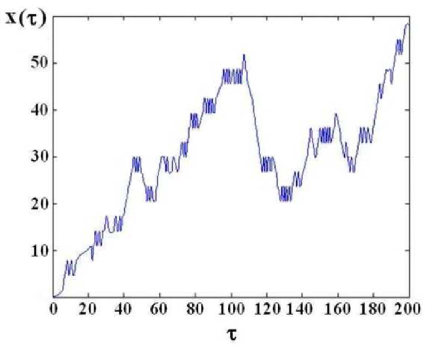
Figure 3: Color online. The chaotic motion of the atom inside the cavity in the regime of a weak coupling. The numerical integration of eqs. (II) is performed for the following values of the parameters $\delta=-0.5$, $\alpha=0.5$, $N=50$, $s=1$, $x(0)=0$, $p(0)=1$,$u(0)=0$, $v(0)=0$, $s_{z}(0)=1$. As evident from the figure, the motion in the nonadiabatic case is chaotic and resembles a diffusion process.

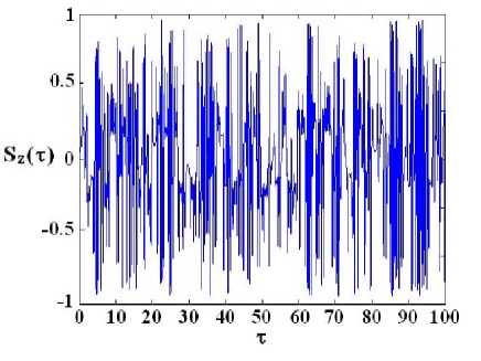
Figure 4: Color online. The dynamics of the atomic inversion as deduced from the numerical integration of eqs.(II) for the following parameters values: $\delta=-0.5$, $\alpha=0.5$, $N=50$, $s=1$, $x(0)=0$, $p(0)=1$,$u(0)=0$, $v(0)=0$, $s_{z}(0)=1$. Obviously the inter-level transitions are of a chaotic nature.

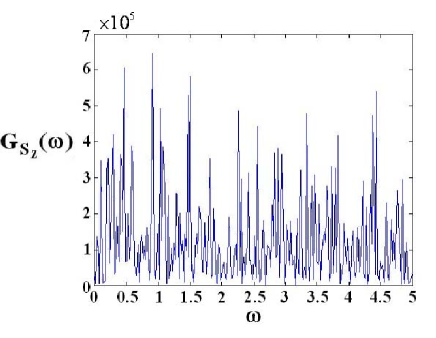
Figure 5: The correlation function for the atomic inversion as delivered by the numerical integration of eqs.(II) for $\delta=-0.5$, $\alpha=0.5$, $N=50$, $s=1$, $x(0)=0$, $p(0)=1$,$u(0)=0$, $v(0)=0$, $s_{z}(0)=1$. The finite width of the correlation function signifies the dynamical stochasticity.

To confirm the existence of chaos, we examine the width of Fourier transform of the correlation function $G_{s_{z}}(\tau^{\prime})=\langle s_{z}(\tau+\tau^{\prime})|s_{z}(\tau)\rangle$, $G_{s_{z}}=\int\limits_{-\infty}^{+\infty}d\tau G_{s_{z}}(\tau)\exp[i\omega\tau]=\frac{\tau_{c}}{1+\omega^{2}\tau_{c}^{2}}$. With $\langle\ldots\rangle=\lim\limits_{T\rightarrow\infty}\frac{1}{T}\int\limits_{0}^{+\infty}(\ldots)dt$ we mean the averaging with respect to time, while $\tau_{c}$ being the correlation time. The result of numerical calculations is presented in Fig.5. The finite width of the Fourier transform signifies the emergence of chaos. The numerical results presented in Figs.3-5 confirm that in the limit of weak coupling $\alpha=\frac{k_{f}^{2}}{m\Omega_{0}}\sim 1$ the dynamics turns chaotic. In contrast, in the limit of a strong coupling chaos appears only in a small area near to the separatrix, as quantified by eq.(40). For nonzero DSS the dynamics is integrable in both cases: for the resonant case $\omega_{0}=\omega_{f}+\frac{\zeta}{2}$ (9) and for the non-resonant case $\omega_{0}\neq\omega_{f}+\frac{\zeta}{2}$ (26).

Summarizing this part of the work, we found that when the detuning between the radiation field and the spin splitting is larger than DSS $\omega_{f}-\omega_{0}>\zeta$ two different types of dynamics are realized: 1) In the regime of a strong coupling between the atom and the cavity $\alpha=\frac{k_{f}^{2}}{m\Omega_{0}}\ll 1$ the dynamics is regular in the whole phase space, except for a narrow energy gap near to the classical separatrix $|E-E_{s}|<\delta E_{s}$ (cf. Eqs. (39), Eq.(40)). 2) In the regime of a weak coupling $\alpha\sim 1$ almost the whole phase space shows chaotic dynamics. Due to the impact of the spatial motion on the spin dynamics, the spectrum of the inter-level transitions is chaotic as well (see Fig.4).

If the mean photon number in the cavity is not large, then the semi-classical approximation is not justified and the problem should be considered quantum-mechanically. A relevant question in this case is the quantum correlation within the compound quantum systems, i.e. between the atom and the radiation field. The entanglement between the atom and the field is usually quantified in terms of purity Uleysky ; Argonov . As entanglement is a specific quantum form of correlation it exhibits a number of essential differences to classical correlations. These issues will be the subject of the next section.

VI Entanglement between the field and the atom: Quantum mechanical consideration

As was mentioned above, if the mean photon number inside the cavity is not a large number, then a semi-classical treatment is not viable and one should resort to quantum mechanics Uleysky ; Argonov . Having said that, the translational degrees of freedom can still be treated classically; the inter-level transitions are described quantum mechanically, however. Thus, the center-of-mass coordinate of the atom $x(t)$ may still be described by the classical Hamilton’s equations of motion

$$\dot{x}=\alpha p,~{}~{}~{}~{}\dot{p}=-\langle\hat{u}\rangle\sin x.$$ (41)

The quantum mechanical average should be performed then, i.e.

$$\langle\hat{u}\rangle=\bigg{\langle}\frac{1}{\sqrt{N}}\big{(}e^{i\delta t}s^{+}a^{2}+e^{-i\delta t}s^{-}(a^{+})^{2}\big{)}\bigg{\rangle}.$$ (42)

The average is taken with respect to the wave functions that solve for the Schrödinger equation

$$i\frac{d|\psi(t)\rangle}{dt}=\hat{H}_{int}|\psi(t)\rangle.$$ (43)

Here

$$\hat{H}_{int}=\zeta\hat{a}^{+}\hat{a}s_{z}+g(x)\big{(}e^{i\delta t}s^{+}\hat{a}^{2}+e^{-i\delta t}s^{-}(\hat{a}^{+})^{2}\big{)},~{}~{}~{}~{}\delta=\omega_{0}-2\omega_{f}.$$ (44)

Following the standard procedure of Ref. Schleich , we seek solutions of the equation (43) in the form

$$|\psi(t)\rangle=\sum\limits_{n}\bigg{[}C_{e,n}(t)|e,n\rangle+C_{g,n+2}(t)|g,n+2\rangle\bigg{]}.$$ (45)

Substituting eq. (45) into eq. (43) we find a set of equations for determining the expansion coefficients

$$i\dot{C}_{e,n} = \zeta\frac{n}{2}C_{e,n}+g(x)\sqrt{(n+1)(n+2)}e^{-i\delta t}C_{g,n+2},$$

$$i\dot{C}_{g,n+2} = -\zeta\frac{n+2}{2}C_{g,n+2}+g(x)\sqrt{(n+1)(n+2)}e^{i\delta t}C_{e,n}.$$ (46)

In order to derive analytical results for the degree of entanglement we will study the eqs. (VI) in two different limits: For a strong atom-cavity coupling $\alpha=\frac{k_{f}^{2}}{m\Omega_{0}}\ll 1$, the quantity $x(t)$ is an adiabatic variable on the time scale set by the inverse Rabi frequencies. In this case system, as described by eqs. (VI), is exactly solvable and the solutions are given by the following expressions

$$C_{e,n}(t) = e^{i\frac{(\delta-\zeta)t}{2}}\Big{\{}-\frac{ib(n)}{\lambda_{n}}\sin(\lambda_{n}t)C_{g,n+2}(0)+\bigg{(}\cos(\lambda_{n}t)-\frac{i(\delta+\zeta(n+1))\sin(\lambda_{n}t)}{2\lambda_{n}}\bigg{)}C_{e,n}(0)\Big{\}},$$

$$C_{g,n+2}(t) = e^{-i\frac{(\delta+\zeta)t}{2}}\Big{\{}-\frac{ib(n)}{\lambda_{n}}\sin(\lambda_{n}t)C_{e,n}(0)+\bigg{(}\cos(\lambda_{n}t)+\frac{i(\delta+\zeta(n+1))\sin(\lambda_{n}t)}{2\lambda_{n}}\bigg{)}C_{g,n+2}(0)\Big{\}},$$

$$b(n) = g(x)\sqrt{(n+1)(n+2)},~{}~{}~{}\lambda_{n}=\frac{\sqrt{(\delta+\zeta(n+1))^{2}+4b^{2}(n)}}{2}.$$ (47)

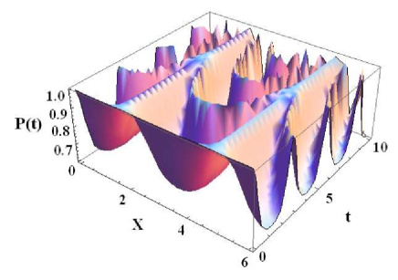
Figure 6: Color online. The purity $P(t)$ as a function of time $t$ and of the center-of-mass position of the atom, as dictated by eq. Eq.(51). The following parameters have been chosen $\Omega_{0}=1$ ,$\bar{n}=1$, $\zeta=1$.

Using these solutions and after tracing out the field’s degrees of freedom one can introduce the reduced density matrix for the atomic subsystem as

$$\rho^{a}=\left(\begin{array}[]{c}\rho_{11}^{a}~{}~{}~{}\rho_{12}^{a}\\ \rho_{21}^{a}~{}~{}~{}\rho_{22}^{a}\end{array}\right),$$ (48)

where

$$\rho_{11}^{a} = \sum\limits_{n}\bigg{|}C_{e,n}(t)\bigg{|}^{2},~{}~{}~{}\rho_{12}^{a}=\sum\limits_{n}C_{e,n}(t)C^{*}_{g,n+2},$$

$$\rho_{21}^{a} = \sum\limits_{n}C_{g,n+2}^{*}(t)C_{e,n},~{}~{}~{}\rho_{22}^{a}=\sum\limits_{n}\bigg{|}C_{g,n+2}(t)\bigg{|}^{2},$$ (49)

$$C_{e,n}(0) = c_{e}W_{n},~{}~{}~{}C_{g,n+2}(0)=c_{g}W_{n+2},c_{e}=1,c_{g}=0.$$

Here $W_{n}^{2}=\frac{\bar{n}^{n}}{n!}e^{-\bar{n}}$ is the distribution function of the field coherent states Schleich . Substituting eq.(VI) in eq.(VI) we conclude the following explicit form for the elements of the reduced density matrix (48) $(\omega_{0}=2\omega_{f}+\zeta,n\gg 1)$:

$$\rho_{11}^{a} = \frac{1}{2}\bigg{(}1+e^{-\bar{n}(1-\cos(2t\lambda))}\cdot\cos(\bar{n}\sin(2t\lambda)\bigg{)}+$$

$$+ \frac{1}{2}\frac{\zeta^{2}}{4\lambda^{2}}\bigg{(}1-e^{-\bar{n}(1-\cos(2t\lambda))}\cdot\cos(\bar{n}\sin(2t\lambda)\bigg{)},$$

$$\rho_{12}^{a} = -\frac{ig(x)}{2\lambda}e^{-i\zeta t}e^{-\bar{n}(1-\cos(2t\lambda))}\sin(\bar{n}\sin(2t\lambda)+$$

$$+ \frac{1}{2}e^{-i\zeta t}\cdot\frac{g(x)\zeta}{2\lambda^{2}}\bigg{(}1-e^{-\bar{n}(1-\cos(2t\lambda))}\cdot\cos(\bar{n}\sin(2t\lambda)\bigg{)},$$

$$\rho_{21}^{a} = \frac{ig(x)}{2\lambda}e^{i\zeta t}e^{-\bar{n}(1-\cos(2t\lambda))}\sin(\bar{n}\sin(2t\lambda)+$$

$$+ \frac{1}{2}e^{i\zeta t}\cdot\frac{g(x)\zeta}{2\lambda^{2}}\bigg{(}1-e^{-\bar{n}(\cos(2t\lambda)-1)}\cdot\cos(\bar{n}\sin(2t\lambda)\bigg{)},$$

$$\rho_{22}^{a} = \frac{1}{2}\frac{g^{2}(x)}{\lambda^{2}}\bigg{(}1-e^{-\bar{n}(1-\cos(2t\lambda))}\cdot\cos(\bar{n}\sin(2t\lambda)\bigg{)},$$

$$\lambda^{2} = \bigg{(}\frac{\zeta}{2}\bigg{)}^{2}+g^{2}(x).$$

The interaction between the atom and the radiation field is described by the nonseparable wave function (45), i.e. by an entangled state Schleich . The entanglement between the atom and the field has a different meaning from the usual definition of the entanglement between the atomic states. The field is the subsystem with a large number of degrees of freedom and is usually prepared in a coherent state. Therefore, the state of the field is not influenced by the atom-field coupling interaction. For quantifying the entanglement between the atom and the field we should average and trace out the field’s states on the cost of a partial loss of coherence. To make this point clear, let us consider the simplest protocol of a quantum measurement Schleich . The probability $W(t,|\psi_{a}(t)\rangle,|\psi_{field}(t)\rangle)$ that both subsystems are in the particular states $|\psi_{a}(t)\rangle$ and $|\psi_{field}(t)\rangle$ is defined via the following relation:

$$W(t,|\psi_{a}(t)\rangle,|\psi_{field}(t)\rangle)=|\langle\psi_{field}\mid\langle\psi_{a}\mid\psi(t)\rangle|^{2},$$ (51)

$$\mid\psi(t)\rangle=\sum\limits_{n}\sum\limits_{j=e,g}\psi_{jn}(t)\mid j,n\rangle.$$ (52)

Here

$$\psi_{en}(t)=C_{en}(t),~{}~{}~{}\psi_{gn}(t)=C_{g,n+2}(t).$$ (53)

As simple quantum measurement one may perform on the system is that, one observes the atomic state for an arbitrary field state. As we already have mentioned above, the field is prepared in a coherent state Schleich . The entanglement between the atom and the field (while statistically averaging over the field states) is quantified in terms of the purity $P$ Bruss

$$P\big{(}t,\mid\psi_{a}\rangle\big{)}=\sum\limits_{n=0}\limits^{\infty}\mid\sum\limits_{j=e,g}\psi_{jn}(t)\langle\psi_{a}\mid j,n\rangle\mid^{2}.$$ (54)

Comparing eq. (54) with eq. (51) we conclude on a partial loss of coherence, since some interference terms are omitted in eq.(54). Nevertheless, the atomic and the field subsystems are still entangled and the density operator of the total system cannot be written as a direct product of density operators each corresponding to the atom and the field subsystems Using eqs. (49, 53 and 54) the purity of the quantum state is expressible in terms of the reduced density matrix in the standard form Bruss , meaning that

$$P\big{(}t,\mid\psi_{a}\rangle\big{)}=P(t)=Tr\bigg{(}\big{(}\rho^{a}\big{)}^{2}\bigg{)}=\big{(}\rho^{a}_{11}\big{)}^{2}+\big{(}\rho_{22}^{a}\big{)}^{2}+2\rho_{12}^{a}\rho_{21}^{a}=$$

$$=1-\frac{g^{2}(x)}{\lambda^{2}}\big{\{}1-\exp\big{[}-2\bar{n}\big{(}1-\cos(2t\lambda)\big{)}\big{]}\big{\}},$$ (55)

$$0<P(t)<1.$$

From eq.(55) we readily deduce that the degree of coherence degrades with the decrease of DSS. The purity as a function of time and of the adiabatic coordinate is plotted in Fig.6. The purity is distributed non-uniformly, since the Rabi frequencies are coordinate dependent (VI). In the semi-classical limit, when the mean photon number in the cavity is large $\bar{n}\gg 1$, the expression given by eq. (55) simplifies and for the time- and the coordinate-averaged purity we obtain $P=\bigg{(}1-\frac{2\Omega_{0}^{2}}{\zeta^{2}+4\Omega_{0}^{2}}\bigg{)}$. We see that the ratio of the cavity-atom coupling constant and the DSS $\Omega_{0}/\zeta$ is still the determining factor in our problem. From the expression above, the maximum of the purity is $P_{max}=1$ for the case $\Omega_{0}/\zeta\ll 1$ and $P_{min}=\frac{1}{2}$ for $\Omega_{0}/\zeta\gg 1$, respectively. In the opposite case corresponding to the weak atom-cavity coupling with $\alpha=\frac{k_{f}^{2}}{m\Omega_{0}}\sim 1$, the analytical solution of the system (VI) can be found in the special case of a resonant driving $\delta=\omega_{0}-2\omega_{f}=0$

$$C_{e,n} = \exp\bigg{(}-\frac{in\zeta t}{2}\bigg{)}\bigg{(}C_{1}Q[n\omega(t)]+C_{2}Q^{*}[n\omega(t)]\bigg{)},$$

$$C_{g,n+2} = \exp\bigg{(}\frac{i(n+1)\zeta t}{2}\bigg{)}\bigg{(}C_{1}Q[n\omega(t)]-C_{2}Q^{*}[n\omega(t)]\bigg{)},$$ (56)

where

$$C_{1}=\frac{C_{e,n}(0)+C_{g,n+2}(0)}{2},~{}~{}~{}C_{2}=\frac{C_{e,n}(0)-C_{g,n+2}(0)}{2},$$ (57)

and

$$Q[n\omega(t)]=\exp\Big{[}in\int\limits_{0}^{t}\omega(t^{\prime})dt^{\prime}\Big{]},~{}~{}~{}Q^{-1}[\omega]=Q^{*}[\omega],~{}~{}~{}\omega(\tau)=\cos(x(\tau)).$$ (58)

From eqs.(VI, 57) we infer for the reduced density matrix and its purity the following forms

$$P(t)=Tr\bigg{(}\big{(}\rho^{a}\big{)}^{2}\bigg{)}=\big{(}\rho^{a}_{11}\big{)}^{2}+\big{(}\rho_{22}^{a}\big{)}^{2}+2\rho_{12}^{a}\rho_{21}^{a}$$ (59)

$$0<P(t)<1.$$

The explicit forms of the density matrix elements are

$$\rho_{11}^{a} = \sum\limits_{n}\bigg{[}C_{1}^{2}+C_{2}^{2}+C_{1}C_{2}\big{(}Q^{*2}\big{[}n\omega(t)\big{]}+Q^{2}\big{[}n\omega(t)\big{]}\big{)}\bigg{]},$$

$$\rho_{12}^{a} = \sum\limits_{n}\bigg{[}C_{1}^{2}-C_{2}^{2}+C_{1}C_{2}\big{(}Q^{*2}\big{[}n\omega(t)\big{]}-Q^{2}\big{[}n\omega(t)\big{]}\big{)}\bigg{]},$$

$$\rho_{21}^{a} = \sum\limits_{n}\bigg{[}C_{1}^{2}-C_{2}^{2}+C_{1}C_{2}\big{(}Q^{2}\big{[}n\omega(t)\big{]}-Q^{*2}\big{[}n\omega(t)\big{]}\big{)}\bigg{]},$$ (60)

$$\rho_{22}^{a} = \sum\limits_{n}\bigg{[}C_{1}^{2}+C_{2}^{2}-C_{1}C_{2}\big{(}Q^{*2}\big{[}n\omega(t)\big{]}+Q^{2}\big{[}n\omega(t)\big{]}\big{)}\bigg{]}.$$

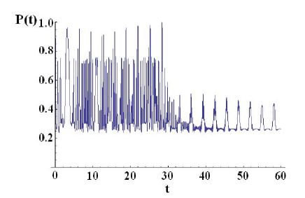
Figure 7: Color online. The purity $P(t)$ as a function of time $t$, as described by Eqs.(55, 57, 58). The following parameter are chosen: $\alpha=10^{-2}$ $\bar{n}=1$, $\zeta=0.2$, $\Omega_{0}=0.1$.

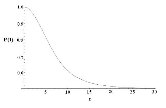
Figure 8: The purity $P(t)$ as a function of the time $t$. The results follow from Eqs.(55, 57, 61). In the calculations the following parameters are chosen $\alpha=0.5$ $\bar{n}=1$, $\zeta=0.2$, $\Omega_{0}=0.1$, $\alpha_{0}=1$.

Considering the initial conditions (57), and tracing over the field states in eq. (VI), we obtain for matrix elements

$$\rho_{11}^{a} = \frac{1}{2}+\frac{1}{4}e^{-\bar{n}}\bigg{(}e^{\bar{n}Q[2\omega[t]]}+e^{\bar{n}Q^{*}[2\omega[t]]}\bigg{)},$$

$$\rho_{22}^{a} = \frac{1}{2}-\frac{1}{4}e^{-\bar{n}}\bigg{(}e^{\bar{n}Q[2\omega[t]]}+e^{\bar{n}Q^{*}[2\omega[t]]}\bigg{)},$$ (61)

$$\rho_{12}^{a} = \frac{1}{4}e^{-\zeta i}\bigg{(}e^{\bar{n}Q^{*}[2\omega(t)]\exp(-it\zeta)}-e^{\bar{n}Q[2\omega(t)]\exp(-it\zeta)}\bigg{)}e^{-\bar{n}},$$

$$\rho_{21}^{a} = \frac{1}{4}e^{\zeta i}\bigg{(}e^{\bar{n}Q[2\omega(t)]\exp(it\zeta)}-e^{\bar{n}Q^{*}[2\omega(t)]\exp(it\zeta)}\bigg{)}e^{-\bar{n}}.$$

The time dependence of the matrix elements of the reduced density matrix, as given by eqs. (VI, VI), is governed by the exponential factors (58). We evaluate $Q[2\omega(t)]$ for two different regimes. In the regime of a regular motion, using solution (24) we simply have

$$Q\big{[}2\omega(t)\big{]}\approx\exp\Big{[}2i\sqrt{\frac{\Omega_{0}}{\alpha\zeta}}\big{[}Ci(e^{t\sqrt{\frac{\alpha\zeta}{\Omega_{0}}}})-Ci(1)\big{]}\Big{]},$$ (62)

where $Ci(\ldots)$ is the cosine integral function Abramowitz . In this case the purity exhibits fast oscillations, as evidenced by Fig.7. From Fig.7 we conclude that after a lap of time $t=t_{c}\approx 50$, the oscillation frequency decreases. The reason for this behavior can be traced back to the time dependency of the parameters given by eq. (58) (i.e., $Q\big{[}2\omega(t)\big{]}$): For $t>t_{c}$, $Q\big{[}2\omega(t)\big{]}\approx\exp\big{[}-2i\sqrt{\frac{\Omega_{0}}{\alpha\zeta}}Ci(1)\big{]}=const$ and the diagonal elements of the density matrix are constant in time

$$\rho^{a}_{11}=\frac{1}{2}+\frac{1}{2}\exp(-\bar{n})\cos\big{(}\bar{n}\exp\big{[}2\sqrt{\frac{\Omega_{0}}{\alpha\zeta}}Ci(1)\big{]}\big{)},$$ (63)

$$\rho^{a}_{22}=\frac{1}{2}-\frac{1}{2}\exp(-\bar{n})\cos\big{(}\bar{n}\exp\big{[}2\sqrt{\frac{\Omega_{0}}{\alpha\zeta}}Ci(1)\big{]}\big{)}.$$ (64)

Hence, $\big{(}\rho_{11}^{a}\big{)}^{2}+\big{(}\rho_{22}^{a}\big{)}^{2}=const$ and the temporal dependence of the purity is governed by the off-diagonal term $2\rho_{12}^{a}\rho_{21}^{a}$. In the semi-classical limit $\bar{n}\gg 1$ the purity turns constant $P=1/2$ and is independent of the values of the frequency shift. In the regime when the motion is chaotic, we use a more advanced technique for the evaluation of $Q[\omega(t)]$. Namely, because of the random character of the atomic motion, the exponent, given by eq. (58), should be considered as a functional of the random function $\omega(t)$. Therefore, we should carry out a statistical average with respect to all possible realizations of the random parameters. The mean value of the functional $\langle Q[\omega(t)]\rangle$ can be calculated by evaluating the following integral

$$\langle Q[\omega(t)]\rangle=\exp\Big{[}i\int\limits_{0}^{t}\omega(t^{\prime})dt^{\prime}\Big{]}=\lim\limits_{N\rightarrow\infty\atop\Delta t_{k}\rightarrow 0}\int d\omega_{N}\ldots d\omega_{1}\exp\Big{[}i\sum\limits_{k=1}^{n}\omega_{k}\Delta t_{k}\Big{]}P_{N}[\omega],$$

$$\Delta t_{k}=t^{k}-t^{k-1},~{}~{}~{}t^{0}=0,~{}~{}~{}t^{N}=1.$$ (65)

Here, the multidimensional normal distribution function is given via the expression

$$P_{N}[\omega]=(2\pi)^{-N}\int d\lambda_{1}\ldots d\lambda_{N}\exp\Big{[}-i\sum_{k}\lambda_{k}\omega_{k}\big{]}\exp\Big{[}-\frac{1}{2}\sum\limits_{k,k^{\prime}}C_{kk^{\prime}}\lambda_{k}\lambda_{k^{\prime}}\Big{]},$$ (66)

where $\lambda_{k}$ are distribution parameters and $C_{kk^{\prime}}$ is the covariation matrix Feller . Substituting eq. (66) in eq. (VI) and performing the integration we obtain

$$\langle Q[\omega(t)]\rangle\approx\exp\Big{[}-\frac{t}{2}\sqrt{\frac{\pi}{\alpha_{0}}}Erf\bigg{[}t\sqrt{\alpha_{0}}\bigg{]}\Big{]},$$ (67)

where $Erf[\ldots]$ is the error function, and $1/\alpha_{0}$ is the width of the correlation function
$c(\tau)=\langle\omega(t+\tau)\omega(t)\rangle$. Taking eqs. (VI-67) into account one can evaluate the time dependence of the purity in both the regular and the chaotic cases. The result of the numerical calculations is presented in Fig.(8). As we see, after a fast decay, the purity stabilizes around the value $P(t)\sim 0.5$. The corresponding decay rate is determined by the correlation width $1/\alpha_{0}$ of the random parameter $x(t)$.

VII Conclusions

In the present paper, our aim was to analyze the dynamics of the TC atom in a non-uniform cavity, in order to uncover the consequences of the DSS for the weak and the strong cavity-field couplings. We found that in the regime of a strong coupling $\alpha=\frac{k_{f}^{2}}{m\Omega_{0}}\ll 1$, the motion of the atom inside the cavity is adiabatic. For the case when an exact resonance is reached $\zeta=2(\omega_{0}-\omega_{f})$, then depending on the values of the center of mass coordinate of the atom $x(t)$, the level populations are described by topologically distinct solutions separated by a bifurcation parameter. The motion of the atom inside the non-uniform cavity leads to a tunneling of the system through the separatrix and as a consequence to singularities in the inter-level transition spectrum $S_{z}(t)$. The bifurcation point is identified by a simple analytical expression, given by eq.(25). A key factor is the relationship between DSS and the atom-cavity coupling constant $\zeta/\Omega_{0}$. Therefore, by observing the singularity in the spectrum of the Rabi oscillations of the inter-level transitions $S_{z}(t)$ one may infer the frequency shift in an indirect way. Far from the resonance $\zeta>>2(\omega_{0}-\omega_{f})$, the spatial motion of the atom inside the cavity leads to a switching of the spin projection between the values $S_{z}=1$ and $S_{z}=1/2$. The period of switching depends on the values of DSS: $T=\frac{\pi}{2(R_{0}cos(x)+g)},~{}g=\frac{\zeta}{\Omega_{0}}+\frac{\omega_{f}-\omega_{0}}{\Omega_{0}}$. In the regime of a weak coupling $\alpha=\frac{k_{f}^{2}}{m\Omega_{0}}\sim 1$, the motion of the atom inside the cavity becomes chaotic (see Fig. 3-5). We find that, in the adiabatic case, the ratio of the cavity-atom coupling constant and the DSS $\Omega_{0}/\zeta$ are still the determining factors. Namely, in the semi-classical limit, when the mean photon number in the cavity is large $\bar{n}>>1$, the time and the coordinate-averaged purity is $P=\bigg{(}1-\frac{2\Omega_{0}^{2}}{\zeta^{2}+4\Omega_{0}^{2}}\bigg{)}$. Therefore, the maximum of the purity $P_{max}=1$ is achieved for the case $\Omega_{0}/\zeta<<1$ and $P_{min}=\frac{1}{2}$ corresponds to the case $\Omega_{0}/\zeta>>1$.

Acknowledgments The financial support by the Deutsche Forschungsgemeinschaft (DFG) through SFB 762, the HGSFP (grant number GSC 129/1), the Heidelberg Center for Quantum Dynamics, grant No. KO-2235/3 and STCU grant No 5053 is gratefully acknowledged.

References

• (1) T. Aoki et al, Nature 443, 671 (2006).
• (2) H. Mabuchi, A. Doherty, Science 298, 1372 (2002).
• (3) C.J. Hood et al, Science 287, 1447 (2000).
• (4) J. Raimond, M. Brune, S. Haroche, Rev. Mod. Phys. 73, 565 (2001).
• (5) S. N. Shevchenko, S. Ashhab, F. Nori, Phys. Reports 492, 1 (2010).
• (6) K. Maruyama, F. Nori, V. Vedral, Rev. Mod. Phys. 81, 1 (2009).
• (7) I. Buluta, F. Nori, Science 326, 108 (2009).
• (8) L. Amico, R. Fazio, A. Osterloh, V. Vedral, Rev. Mod. Phys. 80, 517 (2008).
• (9) F. Mintert, A. Carvalho, M. Kus, A. Buchleitner, Phys. Rep. 415, 207 (2005).
• (10) D. Bruss and G. Leuchs, Lectures on Quantum Information Wiley-VCH Verlag, Weinheim (2007); D. Witthaut, F. Trimborn, and S. Wimberger, Phys. Rev. Lett. 101, 200402 (2008).
• (11) E. Jaynes, F. Cummings, Proc. IEEE 51, 89 (1963).
• (12) P. Schleich, Quantum Optics in Phase Space, Wiley-VCH, Berlin, (2001).
• (13) S.V. Prants, M. Edelman, G.M. Zaslavsky, Phys. Rev. E 66, 046222 (2002).
• (14) L. Chotorlishvili, Z. Toklikishvili, Eur. Phys. J. D 47, 433 (2008); Phys. Lett. A 372, 2806 (2008); N. Metwally, L. Chotorlishvili, V. Skrinnikov, Physica A. 389, 5332 (2010).
• (15) A. Joshi, R.R. Puri, J. Mod. Opt. 36, 215 (1989).
• (16) A. Rybin, G. Kastelewicz, J. Timonen, N. Bogoliubov, J. Phys. A Math. Gen. 31, 4705. (1998).
• (17) M. Brune, J. M. Raimond, S. Haroche, Phys. Rev. A 35, 154 (1986).
• (18) E. Jahnke, F. Emde, F. Lösch, Tafeln Höherer Funktionen, B. G. Teubner Verlagsgesellschaft, Stuttgart (1960), M. Abramowitz and Stegun I (ed) Handbook of Mathematical Functions (Applied Mathematics Series vol 55) (Washington: National Bureau of Standards)(1972).
• (19) G. M. Zaslavsky, The Physics of Chaos in Hamiltonian Systems 2nd edn (London: Imperial College) (2007).
• (20) N.V. Butenin, Y.I. Nejmark, and N.A. Fufaev, Introduction to the Theory of Nonlinear Oscillations, Nauka, Moscow, (in Russian) (1987).
• (21) S. V. Prants and M.Yu. Uleysky, Phys. Lett. A 309, 357 (2003).
• (22) S. V. Prants, M. Yu. Uleysky, and V. Yu. Argonov, Phys. Rev. A 73, 023807 (2006).
• (23) W. Feller, An Introduction to Probability Theory and Its Applications, vol. 1, John Wiley and Sons, New York, (1958).
W. Feller, An Introduction to Probability Theory and Its Applications, vol. 2, John Wiley and Sons, New York, (1966).