Vortex formation in a rotating two-component Fermi gas

Abstract

A two-component Fermi gas with attractive $s$-wave interactions forms a superfluid at low temperatures. When this gas is confined in a rotating trap, fermions can unpair at the edges of the gas and vortices can arise beyond certain critical rotation frequencies. We compute these critical rotation frequencies and construct the phase diagram in the plane of scattering length and rotation frequency for different total number of particles. We work at zero temperature and consider a cylindrically symmetric harmonic trapping potential. The calculations are performed in the Hartree-Fock-Bogoliubov approximation which implies that our results are quantitatively reliable for weak interactions.

I Introduction

A characteristic feature of superfluids is the appearance of vortices when they are rotated. This fact has been used to demonstrate that a two-component atomic Fermi gas becomes a superfluid at sufficiently low temperatures Zwierlein05 ; Zwierlein06 ; Zwierlein06b ; Schunck07 . A superfluid state can be created in such a gas by trapping fermionic atoms in two distinct hyperfine states. The interaction strength between the two components can be controlled by an external magnetic field. When the interactions are tuned to be attractive, and the atoms are cooled to sufficiently low temperatures, the components will form pairs via the Cooper instability. Due to this pair formation the Fermi gas becomes a Bardeen-Cooper-Schrieffer (BCS) superfluid as was envisaged in Refs. Stoof96 ; Houbiers97 .

The response of the superfluid to rotation can be investigated by rotating the trapping potential with a certain frequency $\Omega$. For a non-rotating trap the entire gas will form a superfluid without vortices. Let us now imagine increasing the rotation frequency at zero temperature. Up to a certain critical rotation frequency, the superfluid will stay in the vortex-free state carrying zero angular momentum. For low temperatures the angular momentum will be quenched, as has also been observed experimentally AngularMomentumQuenching . Above the critical frequency, angular momentum will be inserted in the gas by either unpairing the fermions near the edges of the gas, by formation of vortices, or by the combination of both effects. The goal of this paper is to compute the rotation frequencies at which these transitions take place.

Besides the experimental investigations Zwierlein05 ; Zwierlein06 ; Zwierlein06b ; Schunck07 ; AngularMomentumQuenching , various theoretical studies of rotating two-component Fermi gases have been performed (for a review see e.g. Ref. Giorgini08 ). The profile of a single vortex was analyzed in this context for the first time in Ref. Rodriguez01 using a Ginzburg-Landau approach and in Ref. Nygaard03 by solving the Bogoliubov-de Gennes equation. In Ref. Bulgac03 it was concluded that a single vortex can induce a sizable density depletion at its core. This was also found to be the case for a vortex lattice Feder04 . Density depletion is important, since it allows the vortices to be detected experimentally Zwierlein05 . The vortex profile was investigated in a population imbalanced gas in Ref. Takahashi06 and in situation in which the two components have unequal mass in Ref. Iskin08 . Real-time dynamics of vortices has been studied in Ref. Bulgac11 .

Vortex lattices in two-component Fermi gases have been examined in several ways in Refs. Feder04 ; Botelho06 ; Tonini08 . At high rotation frequencies a completely unpaired phase is preferred over a vortex lattice. The critical rotation frequency corresponding to this transition was computed in Refs. Zhai06 ; Veillette06 . A vortex lattice can also be destroyed by heating the gas. The corresponding critical temperature was computed in Refs. Feder04 ; Moller07 . When the number of trapped components is unequal, a vortex lattice might be formed within the Fulde-Ferrell-Larkin-Ovchinnikov (FFLO) phase. Its melting temperature was investigated in Ref. Shim06 and its upper critical rotation frequency in Ref. Kulic09 .

The first analysis of the critical frequency $\Omega_{c}$ for vortex formation in a two-component Fermi gas was performed in Ref. Bruun01 . To obtain $\Omega_{c}$ the Helmholtz free energy difference $\Delta F$ between a vortex with unit angular momentum located at the center of the trap and the vortex-free superfluid was estimated at $\Omega=0$. For a cylindrically symmetric infinite well as the trapping potential, $\Delta F$ was obtained by solving the Bogolibuov-de Gennes equation in Refs. Nygaard03 ; Nygaard04 . The free energy difference arises from the loss of condensation energy at the vortex core, the kinetic energy of fermions circulating around the vortex core, and the energy needed to expand the cloud to accommodate the excess particles removed from the vortex core (the latter effect was not considered in Ref. Bruun01 , but was taken into account in Refs. Nygaard03 ; Nygaard04 ). When rotating the trap, the free energy decreases with $\Omega L_{z}$, where $L_{z}$ is the angular momentum contained in the gas. For the vortex-free superfluid $L_{z}=0$, while for the vortex with unit angular momentum $L_{z}=N\hbar/2$, with $N$ the number of trapped particles. These estimates are correct if rotating the trap does not cause unpairing near the edges of the gas. The critical rotation frequency in this case is $\Omega_{c}=2\Delta F/(N\hbar)$. This frequency is similar to the lower critical magnetic field in type-II superconductors Bardeen69 .

Fermions confined in a rotating trap can unpair near the edges Bausmerth08 ; Urban08 ; Iskin09 . This effect was not considered in Refs. Bruun01 ; Nygaard03 ; Nygaard04 . In this paper we will take into account this possibility in order to obtain a more reliable value of $\Omega_{c}$. We will make detailed study of how $\Omega_{c}$ varies with the interaction strength and the number of trapped particles. Furthermore we will compute the critical rotation frequency for unpairing. We consider a cylindrically symmetric harmonic trapping potential. Our calculations are carried out in the Hartree-Fock-Bogoliubov approximation. Therefore, we expect that our results are reliable only in the weak coupling limit.

Let us finally remark that vortices have also been observed in rotating Bose-Einstein condensates (BEC) of bosonic atoms BECvortices and of bosonic dimers composed of fermionic atoms Zwierlein05 (for a review see e.g. Ref. Fetter09 ). The behavior of vortices through the BEC-BCS crossover was investigated experimentally in Ref. Zwierlein05 . In this article we only discuss the BCS regime. A computation of the critical rotation frequency for vortex formation in a BEC is discussed in Ref. Stringari99 . Theoretical studies of behavior of vortices through the BEC-BCS crossover have been performed in Refs. Kawaguchi04 ; Chien06 ; Sensarma06 .

This article is organized as follows. In Sec. II we will introduce the action from which one can derive the properties of the Fermi gas. To achieve this in practice we will adopt the two-particle irreducible (2PI) effective action, which we explain in Sec. III. From the 2PI effective action one obtains the Dyson-Schwinger equation which is the main equation we have to solve. This can be achieved by finding the solution of the Bogoliubov-de Gennes equation, which is explained in Sec. IV. The numerical methods by which we have solved the Bogoliubov-de-Gennes and the Dyson-Schwinger equation are discussed in Secs. V and VI respectively. The reader who is not interested in the details of the calculation can immediately go to Sec. VII where we present the results. The phase diagrams presented in Figs. 14 and 15 are our main results. We draw our conclusions in Sec. VIII. Several details are relegated to the appendices. In Appendix A we review the 2PI effective action. A derivation of the Bogoliubov-de Gennes equation is presented in Appendix B. To solve the Bogoliubov-de Gennes equation numerically, we will use a basis based on Maxwell polynomials. We discuss the computation of the quadrature weights and nodes of these polynomials in Appendix C. In Appendix D we derive the representation of the single particle Hamiltonian in the basis we will employ.

II Setup

Let us consider a two-component Fermi gas in which $s$-wave interactions are dominant and label its components by $\alpha=\uparrow,\downarrow$. Typically in experimental realizations the higher partial waves can be neglected and the superfluidity is driven by attractive $s$-wave interactions. The interactions among the same components can be neglected since the Pauli principle admits $s$-wave interactions only between the different species. We will denote the $s$-wave interaction potential as $V(\boldsymbol{x})$ and specify it below. Under these assumptions the interacting Fermi gas is described by the following action (see e.g. Ref. Stoof ), $S=S_{\mathrm{kin}}+S_{\mathrm{int}}$ where

$$S_{\mathrm{kin}}=\sum_{\alpha=\uparrow,\downarrow}\int\mathrm{d}X\psi_{\alpha}^{*}(X)\left[\hbar\frac{\partial}{\partial\tau}+H(\Omega)-\mu_{\alpha}\right]\psi_{\alpha}(X),$$ (1)

$$\begin{split}S_{\mathrm{int}}&=\frac{1}{2}\sum_{\alpha=\uparrow,\downarrow}\int\mathrm{d}X\int\mathrm{d}Y\,\psi^{*}_{\alpha}(X_{+})\psi^{*}_{-\alpha}(Y_{+})\\ &\quad\quad\quad\quad\times V(\boldsymbol{x}-\boldsymbol{y})\delta(\tau_{x}-\tau_{y})\psi_{-\alpha}(Y)\psi_{\alpha}(X).\end{split}$$ (2)

Here $\psi_{\alpha}(X)$ is the (path-integral) quantum field corresponding to the $\alpha$ component, and $X=(\boldsymbol{x},\tau_{x})$. We write integration over spatial coordinates and imaginary time $\tau$ as $\int\mathrm{d}X\equiv\int_{0}^{\hbar\beta}\mathrm{d}\tau_{x}\int\mathrm{d}^{3}x$ with the inverse temperature $\beta=1/(k_{B}T)$. Here and in the rest of the article $X_{\pm}=(\boldsymbol{x},\tau_{x}\pm\eta)$ and $\eta$ is an infinitesimal small positive number. We have inserted $X_{+}$ and $Y_{+}$ in Eq. (2) in order to maintain the correct ordering of the fields in the path-integral. We will achieve this in a different way for the kinetic term and explain this at the end of Appendix B. Furthermore $-\uparrow$ is equivalent to $\downarrow$, $\mu_{\alpha}$ denotes the chemical potential, and $H(\Omega)$ is the single-particle Hamiltonian. We will assume that the particles are trapped in a potential that is rotating in the $x$-$y$ plane with angular frequency $\Omega$. It is then convenient to perform the calculation in the rotating frame. The single-particle Hamiltonian $H(\Omega)$ in the rotating frame reads (see e.g. Ref. Stoof )

$$H(\Omega)=\frac{\boldsymbol{p}^{2}}{2M}+U(\boldsymbol{x})-\Omega L_{z},$$ (3)

where $M$ is the fermion mass and $L_{z}=xp_{y}-yp_{x}$ is the $z$-component of the angular momentum. The trapping potential $U(\boldsymbol{x})$ realized in experiments is typically harmonic. In this paper we will study a cylindrically shaped trap given by the potential

$$U(\boldsymbol{x})=\frac{1}{2}M\omega^{2}(x^{2}+y^{2}),$$ (4)

which implies confinement in the $x$-$y$ plane, and infinite extension in the $z$-direction. In an experiment this regime can be reached by choosing the trapping frequency in the $z$-direction much smaller than in the $x$-$y$-direction. In cylindrical coordinates, $\boldsymbol{x}=(\rho\cos\phi,\rho\sin\phi,z)$, the single-particle Hamiltonian reads

$$\begin{split}H(\Omega)&=\frac{\hbar^{2}}{2M}\left(-\frac{\mathrm{d}^{2}}{\mathrm{d}\rho^{2}}-\frac{1}{\rho}\frac{\mathrm{d}}{\mathrm{d}\rho}+\frac{L_{z}^{2}}{\hbar^{2}\rho^{2}}-\frac{\mathrm{d}^{2}}{\mathrm{d}z^{2}}\right)\\ &\quad+\frac{1}{2}M\omega^{2}\rho^{2}-\Omega L_{z},\end{split}$$ (5)

where $L_{z}=-\mathrm{i}\hbar\partial/\partial\phi$. The normalized eigenfunctions $\psi^{0}_{nmp_{z}}(\boldsymbol{x})$ of this Hamiltonian can be written as a product of three functions,

$$\psi^{0}_{nmp_{z}}(\boldsymbol{x})=\frac{1}{\sqrt{L}}R_{nm}(\rho)f_{m}(\phi)\mathrm{e}^{\mathrm{i}p_{z}z},$$ (6)

with the radial quantum number $n=0,1,\ldots$, the angular momentum quantum number $m\in\mathbb{Z}$, and the momentum in the $z$-direction $p_{z}=2\pi\hbar n_{z}/L$ with $n_{z}\in\mathbb{Z}$. The constant $L$ denotes the length of the system in the $z$-direction. In this article we will consider the limit $L\rightarrow\infty$. Then $\frac{1}{L}\sum_{n_{z}}=\int\mathrm{d}p_{z}/(2\pi\hbar)$. The function $f_{m}(\phi)$ is a normalized eigenfunction of $L_{z}$ and is given explicitly by

$$f_{m}(\phi)=\frac{1}{\sqrt{2\pi}}e^{\mathrm{i}m\phi}.$$ (7)

The radial eigenfunctions are given by

$$R_{nm}(\rho)=c_{nm}L_{n}^{|m|}(\bar{\rho}^{2})\bar{\rho}^{|m|}e^{-\bar{\rho}^{2}/2},$$ (8)

where $L_{n}^{a}(x)$ denotes the generalized Laguerre polynomial which has degree $n$. Furthermore $\bar{\rho}=\rho/\lambda$ with the harmonic oscillator length $\lambda=(\hbar/M\omega)^{1/2}$. Normalization gives $c_{nm}^{2}=2n!/[\lambda^{2}(n+|m|)!]$. The energy spectrum of $H(\Omega)$ is given by

$$\epsilon^{0}_{nmp_{z}}=\hbar\omega\left(1+2n+|m|\right)-\hbar\Omega m+\frac{p_{z}^{2}}{2M}.$$ (9)

At low enough temperatures and densities, the typical wavelength of the particles will be much longer than the range of the interaction potential. In that case the detailed structure of the potential is unimportant and the only relevant interaction parameter is the scattering length $a$. To perform a calculation in this situation, one can just choose the most convenient potential that has scattering length $a$. Following Ref. Bruun99 we will use the Huang-Yang potential Huang57

$$V(\boldsymbol{r})=g\delta(\boldsymbol{r})\frac{\partial}{\partial r}r,$$ (10)

where the coupling constant $g=4\pi a\hbar^{2}/M$. Pairing between fermions requires attractive interactions, that is $a<0$ and hence $g<0$. Note that the Huang-Yang potential is not equivalent to an ordinary $\delta$-function potential $g\delta(\boldsymbol{r})$, because the derivative operator also acts on the fields in Eq. (2). The advantage of the Huang-Yang potential is that all relevant physical quantities become automatically convergent Bruun99 . Furthermore, the coupling constant does not have to be renormalized so that the foregoing relation between the scattering length and the coupling constant always holds Bruun99 . In the case of an ordinary $\delta$-function potential one will encounter divergences. This will require a regularization prescription and a renormalization of the coupling constant.

In order to perform calculations it is convenient to rewrite the action in the Nambu-Gor’kov basis. For that purpose we introduce the Nambu-Gor’kov fields

$$\Psi(X)=\left(\begin{array}[]{c}\psi_{\uparrow}(X)\\ \psi^{*}_{\downarrow}(X)\end{array}\right),$$ (11)

and write the kinetic part of the action, Eq. (1), as

$$S_{\mathrm{kin}}=-\hbar\int\mathrm{d}X\int\mathrm{d}X^{\prime}\,\Psi^{\dagger}(X)G_{0}^{-1}(X,X^{\prime})\Psi(X^{\prime}),$$ (12)

where the bare inverse Nambu-Gor’kov propagator reads

$$G_{0}^{-1}(X,X^{\prime})=\\ -\frac{1}{\hbar}\left(\begin{array}[]{cc}\hbar\frac{\partial}{\partial\tau}+H(\Omega)-\mu_{\uparrow}&0\\ 0&\hbar\frac{\partial}{\partial\tau}-H(\Omega)^{*}+\mu_{\downarrow}\end{array}\right)\\ \times\delta(X-X^{\prime}).$$ (13)

Here we used the fact that $H(-\Omega)=H(\Omega)^{*}$. In the Nambu-Gor’kov basis the interaction part of the action becomes

$$\begin{split}S_{\mathrm{int}}&=-\sum_{\alpha=\pm}\int\mathrm{d}X\mathrm{d}Y\mathrm{d}X^{\prime}\mathrm{d}Y^{\prime}\,\Psi^{\dagger}(X^{\prime})\sigma_{\alpha}\Psi(X)\\ &\quad\quad\quad\times\Psi^{\dagger}(Y^{\prime})\sigma_{-\alpha}\Psi(Y)\mathcal{V}_{\alpha}(X,Y;X^{\prime},Y^{\prime}),\end{split}$$ (14)

where $\sigma_{+}=\mathrm{diag}(1,0)$ and $\sigma_{-}=\mathrm{diag}(0,1)$. The potential $\mathcal{V}_{\alpha}$ is given by

$$\mathcal{V}_{\alpha}(X,Y;X^{\prime},Y^{\prime})=\frac{1}{4}\Bigl{[}(1+\alpha)\delta(\tau_{x^{\prime}}-\tau_{y})V(\boldsymbol{x}^{\prime}-\boldsymbol{y})\\ +(1\!-\!\alpha)\delta(\tau_{x}\!-\!\tau_{y^{\prime}})V(\boldsymbol{x}-\boldsymbol{y}^{\prime})\Bigr{]}\delta(X_{\alpha}\!-\!X^{\prime})\delta(Y_{-\alpha}\!-\!Y^{\prime}).$$ (15)

Because the Huang-Yang potential contains a derivative operator, we had to introduce several $\delta$-functions in order to separate the potential operator from the quantum fields.

III 2PI effective action

To study the interacting Fermi gas we will compute the resummed propagator $G_{ij}(X,X^{\prime})=-\langle\Psi_{i}(X)\Psi_{j}^{\dagger}(X^{\prime})\rangle$ and the grand potential $\Phi_{G}$ by using the two-particle irreducible (2PI) effective action 2PI . Readers who are not interested in the details of this formalism can immediately continue with Sec. IV where we discuss the Bogoliubov-de Gennes equation which follows from the 2PI effective action.

The 2PI effective action is also known as the Cornwall-Jackiw-Tomboulis formalism and is equivalent to the Luttinger-Ward functional approach LW . It has been applied previously to investigate pairing in atomic gases Haussmann07 and in quark matter CSC2PI .

The main advantage of the 2PI effective action is that it is a functional method which generates the resummed Nambu-Gor’kov propagator and the corresponding grand potential. Here, we will truncate the 2PI effective action at order $g$, which is equivalent to the Hartree-Fock-Bogoliubov approximation. This leads to the well known Bogoliubov-de Gennes equation. Another advantage of the 2PI method is that any truncation can be systematically improved straightforwardly by taking into account higher order diagrams. This is necessary when extending our results to a strongly coupled Fermi gas.

The 2PI effective action reads (see Appendix A for details) 2PI

$$\Gamma[G]=-\mathrm{Tr}\log G^{-1}-\mathrm{Tr}\left(G_{0}^{-1}G-1\right)+\Gamma_{2}[G],$$ (16)

where $\Gamma_{2}[G]$ is the sum of all 2PI diagrams generated from $S_{\mathrm{int}}$ with propagators $G$. The interaction vertex can be directly read off from Eq. (14). We have displayed the Feynman rules for computing the 2PI effective action in Fig. 1. All diagrams contributing to $\Gamma_{2}[G]$ up to order $g^{2}$ are displayed in Fig. 2.

	$=G_{ab}(X,X^{\prime})$
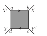
	$\displaystyle{=\sum_{\alpha=\pm}(\sigma_{\alpha})_{ab}(\sigma_{-\alpha})_{cd}\mathcal{V}_{\alpha}(X,Y;X^{\prime},Y^{\prime})}$

Figure 1: Feynman rules for the propagator and the vertex. When connecting propagators to the vertex, the arrows of the propagators have to point in the same direction as the arrows in the vertex. For each closed fermion loop one should include a factor $-1$.

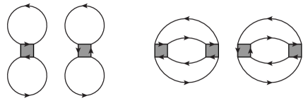
Figure 2: All 2PI diagrams contributing to $\Gamma_{2}[G]$ at order $g$ and order $g^{2}$. Note the direction of the arrows.

By minimizing $\Gamma[G]$ with respect to $G$ one obtains the Dyson-Schwinger equation

$$G^{-1}=G_{0}^{-1}-\Sigma[G],$$ (17)

where the 1PI self-energy is $\Sigma[G]=\delta\Gamma_{2}[G]/\delta G$. The grand potential $\Phi_{G}=-\frac{1}{\beta}\log Z$ is equal to the minimum value of $\Gamma[G]/\beta$ and reads

$$\Phi_{G}=-\frac{1}{\beta}\mathrm{Tr}\log G^{-1}-\frac{1}{\beta}\mathrm{Tr}\left(\Sigma[G]G\right)+\frac{1}{\beta}\Gamma_{2}[G],$$ (18)

where $G$ is now the solution of the Dyson-Schwinger equation, Eq. (17).

In order to perform a practical calculation, one has to truncate $\Gamma_{2}[G]$ at some order. In this paper we will take into account the contributions of order $g$ to $\Gamma_{2}[G]$, which are represented by the first two diagrams in Fig. 2. Such truncation leads to the Hartree-Fock-Bogoliubov approximation. This approximation is expected to give accurate results for small coupling $g$. In general the Hartree-Fock-Bogoliubov approximation can also be applied to strongly correlated systems if the interaction kernel is renormalized appropriately. Such renormalization entails a resummation of ladder diagrams in the Lippman-Schwinger equation. Since we are interested in the weakly interacting BCS limit there is no need to do this.

Applying the Feynman rules to the first two diagrams in Fig. 2 we find that to order $g$, $\Gamma_{2}[G]$ is given by

$$\begin{split}\Gamma_{2}[G]&=-\frac{1}{\hbar}\sum_{\alpha=\pm}\int\mathrm{d}X\mathrm{d}Y\mathrm{d}X^{\prime}\mathrm{d}Y^{\prime}\,\mathcal{V}_{\alpha}(X,Y;X^{\prime},Y^{\prime})\\ &\quad\quad\quad\quad\quad\times\mathrm{tr}\left[G(X,X^{\prime})\sigma_{\alpha}\right]\mathrm{tr}\left[G(Y,Y^{\prime})\sigma_{-\alpha}\right]\\ &\quad+\frac{1}{\hbar}\sum_{\alpha=\pm}\int\mathrm{d}X\mathrm{d}Y\mathrm{d}X^{\prime}\mathrm{d}Y^{\prime}\,\mathcal{V}_{\alpha}(X,Y;X^{\prime},Y^{\prime})\\ &\quad\quad\quad\quad\quad\times\mathrm{tr}\left[G(X,Y^{\prime})\sigma_{\alpha}G(Y,X^{\prime})\sigma_{-\alpha}\right].\end{split}$$ (19)

The relative minus sign arises because the first diagram in Fig. 2 contains two closed loops whereas the second diagram contains only one closed loop when following the arrows.

The self-energy $\Sigma[G]$ can be obtained by differentiating Eq. (19) with respect to $G$. This yields

$$\begin{split}\Sigma[G](X,X^{\prime})&=-\frac{2}{\hbar}\sum_{\alpha=\pm}\sigma_{a}\int\mathrm{d}Y\mathrm{d}Y^{\prime}\,\mathrm{tr}\left[G(Y,Y^{\prime})\sigma_{-\alpha}\right]\\ &\quad\quad\quad\times\mathcal{V}_{\alpha}(X^{\prime},Y;X,Y^{\prime})\\ &\quad+\frac{2}{\hbar}\sum_{\alpha=\pm}\int\mathrm{d}Y\mathrm{d}Y^{\prime}\,\sigma_{\alpha}G(Y,Y^{\prime})\sigma_{-\alpha}\\ &\quad\quad\quad\times\mathcal{V}_{\alpha}(X^{\prime},Y;Y^{\prime},X).\end{split}$$ (20)

The first term is the Hartree self-energy, the second one is the pairing contribution.

The last two equations can be simplified by computing the traces and inserting the explicit expressions for $\mathcal{V}$ and $V(\boldsymbol{r})$. One has then to act the Huang-Yang potential on the propagators. It can be shown Bruun99 that the diagonal components of $G(X,X^{\prime})$ are finite in the limit $r\rightarrow 0$ where $r=|\boldsymbol{x}-\boldsymbol{x}^{\prime}|$. For these components the Huang-Yang potential acts as an ordinary $\delta$-function potential. We will use this fact to simplify the expressions involving the diagonal components of $G$. On the other hand the off-diagonal components of $G$ will have in general a singularity proportional to $1/r$ when $r\rightarrow 0$ Bruun99 . In such situations the full form of the Huang-Yang potential needs to be taken into account.

For later convenience we will now define the pairing field as

$$\Delta(\boldsymbol{x})\equiv\int\mathrm{d}^{3}x^{\prime}\,V(\boldsymbol{x}-\boldsymbol{x}^{\prime})G_{\uparrow\downarrow}(\boldsymbol{x},\tau;\boldsymbol{x}^{\prime},\tau).$$ (21)

Following Ref. Bruun99 we will split the off-diagonal component of the Nambu-Gor’kov propagator into a singular and regular part

$$\lim_{\boldsymbol{x}^{\prime}\rightarrow\boldsymbol{x}}G_{\uparrow\downarrow}(\boldsymbol{x},\tau;\boldsymbol{x}^{\prime},\tau)=\frac{C}{r}+G^{\mathrm{reg}}_{\uparrow\downarrow}(X,X),$$ (22)

where $C$ is some constant and the superscript reg indicates the regular part of $G$. By inserting the Huang-Yang potential in Eq. (21) one can see that the pairing field does not contain any singularity Bruun99

$$\Delta(\boldsymbol{x})=gG^{\mathrm{reg}}_{\uparrow\downarrow}(X,X).$$ (23)

The diagonal components of the propagator can be expressed in terms of number densities. To find the relation between the propagator and the densities we use the definition of the propagator in terms of field operators

$$\begin{split}G_{ij}(X,X^{\prime})&=-\langle T_{\tau}\hat{\Psi}_{i}(X)\hat{\Psi}_{j}^{\dagger}(X^{\prime})\rangle\\ &=\theta(\tau^{\prime}-\tau)\langle\hat{\Psi}_{j}^{\dagger}(X^{\prime})\hat{\Psi}_{i}(X)\rangle\\ &\quad-\theta(\tau-\tau^{\prime})\langle\hat{\Psi}_{i}(X)\hat{\Psi}_{j}^{\dagger}(X^{\prime})\rangle,\end{split}$$ (24)

here $T_{\tau}$ denotes time ordering in imaginary time. Hence the number densities of the two species are related to $G$ as

$$n_{\uparrow}(\boldsymbol{x}) = \langle\hat{\psi}_{\uparrow}^{\dagger}(\boldsymbol{x},\tau)\hat{\psi}_{\uparrow}(\boldsymbol{x},\tau)\rangle=G_{\uparrow\uparrow}(X,X_{+}),$$ (25)

$$n_{\downarrow}(\boldsymbol{x}) = \langle\hat{\psi}_{\downarrow}^{\dagger}(\boldsymbol{x},\tau)\hat{\psi}_{\downarrow}(\boldsymbol{x},\tau)\rangle=-G_{\downarrow\downarrow}(X,X_{-}).$$ (26)

From Eq. (24) it follows that $G_{\uparrow\downarrow}(X,X^{\prime})=\langle\hat{\psi}_{\downarrow}(X^{\prime})\hat{\psi}_{\uparrow}(X)\rangle$ and $G_{\downarrow\uparrow}(X,X^{\prime})=\langle\hat{\psi}^{\dagger}_{\uparrow}(X^{\prime})\hat{\psi}^{\dagger}_{\downarrow}(X)\rangle$. This can be used to show that $G_{\downarrow\uparrow}(X,X^{\prime})=G_{\uparrow\downarrow}(X^{\prime},X)^{*}$ which implies that

$$\begin{split}\Delta(\boldsymbol{x})^{*}&=\int\mathrm{d}^{3}x^{\prime}\,V(\boldsymbol{x}-\boldsymbol{x}^{\prime})G_{\downarrow\uparrow}(\boldsymbol{x},\tau;\boldsymbol{x}^{\prime},\tau)\\ &=gG^{\mathrm{reg}}_{\uparrow\downarrow}(X,X)^{*}.\end{split}$$ (27)

Here we used the fact that the singular part of $G_{\uparrow\downarrow}(X^{\prime},X)^{*}$ is a function of $|\boldsymbol{x}-\boldsymbol{x}^{\prime}|$, so that $\boldsymbol{x}$ and $\boldsymbol{x}^{\prime}$ could be interchanged without changing the result.

We can now use the above definitions to simplify Eqs. (19) and (20). After computing the traces we find that to order $g$, $\Gamma_{2}[G]$ is given by

$$\begin{split}\frac{1}{\beta}\Gamma_{2}[G]&=g\int\mathrm{d}^{3}x\,n_{\uparrow}(\boldsymbol{x})n_{\downarrow}(\boldsymbol{x})\\ &\quad+\int\mathrm{d}^{3}x\,G_{\uparrow\downarrow}(X,X)^{*}\Delta(\boldsymbol{x}).\end{split}$$ (28)

The 1PI self-energy to order $g$ is

$$\Sigma[G](X,X^{\prime})=\frac{1}{\hbar}\left(\begin{array}[]{cc}gn_{\downarrow}(\boldsymbol{x})&\Delta(\boldsymbol{x})\\ \Delta^{*}(\boldsymbol{x})&-gn_{\uparrow}(\boldsymbol{x})\end{array}\right)\delta(X-X^{\prime}).$$ (29)

It follows that $\mathrm{Tr}(\Sigma[G]G)=2\Gamma_{2}[G]+O(g^{2})$ so that the grand potential $\Phi_{G}$, Eq. (18), to order $g$ becomes

$$\begin{split}\Phi_{G}&=-\frac{1}{\beta}\mathrm{Tr}\log G^{-1}-g\int\mathrm{d}^{3}x\,n_{\uparrow}(\boldsymbol{x})n_{\downarrow}(\boldsymbol{x})\\ &\quad-\int\mathrm{d}^{3}x\,G_{\uparrow\downarrow}(X,X)^{*}\Delta(\boldsymbol{x}).\end{split}$$ (30)

Since the particle number in the trap is fixed we solve the equations for the chemical potentials to obtain the desired number of fermions in each hyperfine state. The appropriate thermodynamic potential is then the Helmholtz free energy, which reads

$$F=\Phi_{G}+\mu_{\uparrow}N_{\uparrow}+\mu_{\downarrow}N_{\downarrow},$$ (31)

where $N_{\uparrow,\downarrow}$ denote the total number of particles of a particular species. Since we consider a cylindrically shaped trap, $F$ and $N_{\uparrow,\downarrow}$ are proportional to the length of the trap in the $z$-direction $L$. Since $L$ is taken to be infinite is convenient to consider instead the free energy and particle number per unit of the harmonic oscillator length $\lambda$ in the $z$-direction. For this reason we define

$$\mathcal{F}=\frac{F}{L/\lambda},\;\;\;\;\;\mathcal{N}_{\uparrow,\downarrow}=\frac{N_{\uparrow,\downarrow}}{L/\lambda}.$$ (32)

Furthermore we will define $\mathcal{N}$ to be the total number of particles per unit of length in the $z$-direction, $\mathcal{N}=\mathcal{N}_{\uparrow}+\mathcal{N}_{\downarrow}$.

IV Bogoliubov-de Gennes equation

To proceed, we will insert the explicit expression for the 1PI self-energy, Eq. (29), into Eq. (17). This yields the Dyson-Schwinger equation for the Nambu-Gor’kov propagator,

$$G^{-1}(X,X^{\prime})=-\frac{1}{\hbar}\left(\hbar\frac{\partial}{\partial\tau}+\mathcal{H}\right)\delta(X-X^{\prime}),$$ (33)

with

$$\mathcal{H}=\\ \left(\begin{array}[]{cc}H(\Omega)\!-\!\mu_{\uparrow}\!+\!gn_{\downarrow}(\boldsymbol{x})&\Delta(\boldsymbol{x})\\ \Delta^{*}(\boldsymbol{x})&-H(\Omega)^{*}\!+\!\mu_{\downarrow}\!-\!gn_{\uparrow}(\boldsymbol{x})\end{array}\right).$$ (34)

To solve the Dyson-Schwinger equation, one first inverts both the left- and right-hand sides of Eq. (33). As explained in detail in Appendix B this can be achieved by solving the Bogoliubov-de Gennes equation Gennes64

$$\mathcal{H}\left(\begin{array}[]{c}u_{i}(\boldsymbol{x})\\ v_{i}(\boldsymbol{x})\end{array}\right)=E_{i}\left(\begin{array}[]{c}u_{i}(\boldsymbol{x})\\ v_{i}(\boldsymbol{x})\end{array}\right).$$ (35)

The functions $u_{i}(\boldsymbol{x})$ and $v_{i}(\boldsymbol{x})$ have to be normalized as $\int\mathrm{d}^{3}x\,\left[|u_{i}(\boldsymbol{x})|^{2}+|v_{i}(\boldsymbol{x})|^{2}\right]=1$. Using the explicit expression of $G$, Eq. (105), and Eqs. (25), (26) one can now read off the densities

$$n_{\uparrow}(\boldsymbol{x}) = \sum_{i}f(E_{i})|u_{i}(\boldsymbol{x})|^{2},$$ (36)

$$n_{\downarrow}(\boldsymbol{x}) = \sum_{i}f(-E_{i})|v_{i}(\boldsymbol{x})|^{2},$$ (37)

where $f(E)=[\exp(\beta E)+1]^{-1}$ is the Fermi-Dirac distribution function.

As follows from Eqs. (23) and (105) to obtain $\Delta(\boldsymbol{x})$ we need to extract the regular part of the propagator

$$G_{\uparrow\downarrow}(\boldsymbol{x},\tau;\boldsymbol{x}^{\prime},\tau)=\sum_{i}f(E_{i})u_{i}(\boldsymbol{x})v_{i}^{*}(\boldsymbol{x}^{\prime}),$$ (38)

in the limit $\boldsymbol{x}^{\prime}\rightarrow\boldsymbol{x}$. To do so we will use the method proposed in Ref. Bruun99 with the improvements suggested in Refs. Bulgac02 ; Grasso03 .

The sum over all modes in Eq. (38) is logarithmically divergent for $\boldsymbol{x}=\boldsymbol{x}^{\prime}$. The singular part of $G_{\uparrow\downarrow}$ arises from the modes in the integrand with large negative energy. To obtain the regular part in the limit $\boldsymbol{x}^{\prime}\rightarrow\boldsymbol{x}$ we will first subtract this large energy contribution. For this purpose we define

$$\nu_{c}(\boldsymbol{x})=\sum_{|E_{i}|<E_{c}}f(E_{i})u_{i}(\boldsymbol{x})v_{i}^{*}(\boldsymbol{x}),$$ (39)

where $E_{c}$ denotes an energy cutoff introduced to regulate the logarithmic divergence in $\nu_{c}(\boldsymbol{x})$. The part of $\nu_{c}(\boldsymbol{x})$ dominated by the modes with large negative energies can be approximated as Bruun99 ; Bulgac02 ; Grasso03 $\nu_{HE}(\boldsymbol{x})=-\Delta(\boldsymbol{x})K(\boldsymbol{x},\boldsymbol{x};E_{c})$ with

$$K(\boldsymbol{x},\boldsymbol{x}^{\prime};E_{c})=\sum_{E_{s}<\epsilon_{i}<E_{c}}\frac{\psi_{i}(\boldsymbol{x})\psi^{*}_{i}(\boldsymbol{x}^{\prime})}{2\epsilon_{i}},$$ (40)

where here and below $\psi_{i}(\boldsymbol{x})$ and $\epsilon_{i}$ denote the eigenvectors and eigenvalues of the Hartree-Fock Hamiltonian

$$H_{\mathrm{HF}}=H(\Omega=0)-\mu+gn(\boldsymbol{x}).$$ (41)

Here $\mu=(\mu_{\uparrow}+\mu_{\downarrow})/2$ and $n(\boldsymbol{x})=(n_{\uparrow}(\boldsymbol{x})+n_{\downarrow}(\boldsymbol{x}))/2$. The low-energy cut-off $E_{s}$ in Eq. (40) is arbitrary, except that it should be chosen positive in order to avoid singularities arising from the Fermi surface. As an alternative to introducing a low-energy cutoff, one can add a small imaginary part to $\epsilon_{i}$ as done in Refs. Bruun99 ; Bulgac02 ; Grasso03 . In that case the integrand of $K(\boldsymbol{x},\boldsymbol{x}^{\prime};E_{c})$ has a peak near the Fermi surface, which makes the numerical integration over $p_{z}$ difficult. One can reduce this peak by increasing the magnitude of the imaginary part. However, that will worsen the large negative energy approximation of $\nu_{c}(\boldsymbol{x})$. The low-energy cutoff which we apply here does not suffer from these problems.

Let us next define $\nu_{s}(\boldsymbol{x})\equiv\nu_{c}(\boldsymbol{x})-\nu_{HE}(\boldsymbol{x})$. Because $\nu_{HE}(\boldsymbol{x})$ contains the logarithmic divergent part of $\nu_{c}(\boldsymbol{x})$, the difference $\nu_{s}(\boldsymbol{x})$ is finite, and hence converges for large enough $E_{c}$. There is some freedom in choosing $\nu_{HE}(\boldsymbol{x})$. For example, we could have left out the $gn(x)$ term in the Hartree-Fock Hamiltonian as in Refs. Bruun99 ; Bulgac02 . However, by including this term, $\nu_{HE}(\boldsymbol{x})$ approximates $\nu_{c}(\boldsymbol{x})$ much better, which implies that a much smaller value of $E_{c}$ is sufficient to compute $\nu_{s}(\boldsymbol{x})$ accurately Grasso03 .

Summarizing the discussion above, we found that in the limit $\boldsymbol{x}^{\prime}\rightarrow\boldsymbol{x}$, we can write $G_{\uparrow\downarrow}(\boldsymbol{x},\tau;\boldsymbol{x}^{\prime},\tau)=\nu_{s}(\boldsymbol{x})-\Delta(\boldsymbol{x})K(\boldsymbol{x},\boldsymbol{x}^{\prime};\infty)$. Following Refs. Bulgac02 ; Grasso03 the singular part can now be obtained by making use of the Thomas-Fermi approximation. In the limit $\boldsymbol{x}^{\prime}\rightarrow\boldsymbol{x}$ one finds that

$$K(\boldsymbol{x},\boldsymbol{x}^{\prime};\infty)=K(\boldsymbol{x},\boldsymbol{x};E_{c^{\prime}})\\ -\frac{1}{2}\int_{k<k_{c^{\prime}}(\rho)}\frac{\mathrm{d}^{3}k}{(2\pi)^{3}}\frac{1}{\frac{\hbar^{2}\boldsymbol{k}^{2}}{2M}+\frac{1}{2}M\omega^{2}\rho^{2}-\mu+gn(\rho)+\mathrm{i}\gamma}\\ +\frac{1}{2}\int\frac{\mathrm{d}^{3}k}{(2\pi)^{3}}\frac{\mathrm{e}^{\mathrm{i}\boldsymbol{k}\cdot(\boldsymbol{x}-\boldsymbol{x}^{\prime})}}{\frac{\hbar^{2}\boldsymbol{k}^{2}}{2M}+\frac{1}{2}M\omega^{2}\rho^{2}-\mu+gn(\rho)+\mathrm{i}\gamma}.$$ (42)

Here $\gamma$ is an infinitesimal small positive number and $E_{c^{\prime}}$ is a second energy cutoff that can be chosen different from $E_{c}$. For large enough $E_{c^{\prime}}$ the sum of first two terms in Eq. (42) is convergent. The inhomogeneous wavevector cut-off $k_{c^{\prime}}(\rho)$ can be found from

$$\frac{\hbar^{2}k^{2}_{c^{\prime}}(\rho)}{2M}+\frac{1}{2}M\omega^{2}\rho^{2}-\mu+gn(\rho)=E_{c^{\prime}}.$$ (43)

The last term of Eq. (42) contains the singularity. One can now perform the integration over $k$ analytically, which in the limit $\boldsymbol{x}\rightarrow\boldsymbol{x}^{\prime}$ gives Bulgac02 ; Grasso03

$$G_{\uparrow\downarrow}(\boldsymbol{x},\tau;\boldsymbol{x}^{\prime},\tau)=-\frac{M\Delta(\boldsymbol{x})}{4\pi\hbar^{2}}\frac{1}{|\boldsymbol{x}-\boldsymbol{x}^{\prime}|}+G_{\uparrow\downarrow}^{\mathrm{reg}}(\boldsymbol{x},\tau;\boldsymbol{x},\tau),$$ (44)

where

$$G_{\uparrow\downarrow}^{\mathrm{reg}}(\boldsymbol{x},\tau;\boldsymbol{x},\tau)=\nu_{s}(\boldsymbol{x})-\Delta(\boldsymbol{x})K(\boldsymbol{x},\boldsymbol{x};E_{c^{\prime}})\\ \quad+\frac{\Delta(\boldsymbol{x})M}{2\pi^{2}\hbar^{2}}\left[k_{c^{\prime}}(\rho)-\frac{1}{2}k_{F}(\rho)\log\left(\frac{k_{c^{\prime}}(\rho)+k_{F}(\rho)}{k_{c^{\prime}}(\rho)-k_{F}(\rho)}\right)\right].$$ (45)

Here we have introduced the length of the Fermi wavevector $k_{F}(\rho)$ which can be found from the equation

$$\frac{\hbar^{2}k^{2}_{F}(\rho)}{2M}=\mu-gn(\rho)-\frac{1}{2}M\omega^{2}\rho^{2}-\mathrm{i}\gamma.$$ (46)

To obtain $\Delta(\boldsymbol{x})$ we have to multiply Eq. (45) by $g$ as follows from Eq. (23).

Inserting Eq. (109) into Eqs. (30) and (31) gives the Helmholtz free energy

$$\begin{split}F&=-\sum_{i}\left[\frac{|E_{i}|}{2}+\frac{1}{\beta}\log\left(1+\mathrm{e}^{-\beta|E_{i}|}\right)\right]+\sum_{i}\epsilon_{i}\\ &\quad-\int\mathrm{d}^{3}x\,G_{\uparrow\downarrow}(\boldsymbol{x},\tau;\boldsymbol{x},\tau)^{*}\Delta(\boldsymbol{x})\\ &\quad-g\int\mathrm{d}^{3}x\,n_{\uparrow}(\boldsymbol{x})n_{\downarrow}(\boldsymbol{x})+\mu_{\uparrow}N_{\uparrow}+\mu_{\downarrow}N_{\downarrow}.\end{split}$$ (47)

Although some of the individual terms in the last equation are ultraviolet divergent, their sum, and hence the Helmholtz free energy, is ultraviolet finite. The divergence present in the sum over the eigenvalues of the Bogoliubov-de Gennes matrix is canceled by the sum over the eigenvalues of the Hartree-Fock Hamiltonian and by the logarithmic divergence originating from $G_{\uparrow\downarrow}$. This can be made clearer by expressing $G_{\uparrow\downarrow}$ in terms of $\nu_{s}$ and $K$. One finds

$$\begin{split}F&=-\sum_{|E_{i}|<E_{c}}\left[\frac{|E_{i}|}{2}+\frac{1}{\beta}\log\left(1+\mathrm{e}^{-\beta|E_{i}|}\right)\right]+\sum_{\epsilon_{i}<E_{c}}\epsilon_{i}\\ &\quad+\int\mathrm{d}^{3}x\,K(\boldsymbol{x},\boldsymbol{x};E_{c})|\Delta(\boldsymbol{x})|^{2}-\int\mathrm{d}^{3}x\,\nu_{s}(\boldsymbol{x})^{*}\Delta(\boldsymbol{x})\\ &\quad-g\int\mathrm{d}^{3}x\,n_{\uparrow}(\boldsymbol{x})n_{\downarrow}(\boldsymbol{x})+\mu_{\uparrow}N_{\uparrow}+\mu_{\downarrow}N_{\downarrow}.\end{split}$$ (48)

In the absence of a trapping potential $E_{i}$ is known analytically; then it can be seen that Eq. (48) is ultraviolet finite. As we will see in the next section, $F$ is also finite in the general case.

V Solving the Bogoliubov-de Gennes-equation

In the previous section we have reduced the Dyson-Schwinger equation to a nonlinear equation of the form

$$(\Delta(\boldsymbol{x}),n_{\uparrow,\downarrow}(\boldsymbol{x}),\mathcal{N}_{\uparrow,\downarrow})=F(\Delta(\boldsymbol{x}),n_{\uparrow,\downarrow}(\boldsymbol{x}),\mu_{\uparrow,\downarrow}).$$ (49)

We will now discuss how to compute the function $F$ in practice. In the next section we will solve the Dyson-Schwinger equation.

First we will use the symmetries of our problem to simplify the analysis. For zero rotation frequency the superfluid is in a vortex-free phase. Then, the pairing field $\Delta(\boldsymbol{x})$ will be a function of the radial coordinate $\rho$ only, i.e. $\Delta(\boldsymbol{x})=\tilde{\Delta}(\rho)$, where $\tilde{\Delta}(\rho)\in\mathbb{R}$.

We will assume that the first vortex that appears when increasing the rotation frequency carries one unit of angular momentum and is located at the center of the trap. The pairing field for such vortex has the following form: $\Delta(\boldsymbol{x})=\tilde{\Delta}(\rho)\exp(\mathrm{i}\phi)$. After the single vortex has appeared, a vortex lattice can be formed by further increasing the rotation frequency.

For these reasons we will make the following ansatz for the pairing field

$$\Delta(\boldsymbol{x})=\tilde{\Delta}(\rho)\exp(\mathrm{i}k\phi),$$ (50)

where $k$ is the winding number (unit of angular momentum) of the vortex at the center. Hence the $k=0$ case corresponds to the vortex-free phase. To determine the onset of the vortex phase, we have to compare the Helmholtz free energies with $k=0$ and $k=1$. Because of the cylindrical symmetry of the trap and the fact that a possible vortex is located at the origin, the number densities are a function of $\rho$ only, i.e. $n_{\uparrow,\downarrow}(\boldsymbol{x})=n_{\uparrow,\downarrow}(\rho)$.

In this case the solutions of the Bogoliubov-de Gennes equation, Eq. (35), are of the following form

$$u_{i}(\boldsymbol{x}) = \frac{1}{\sqrt{L}}\mathrm{e}^{\mathrm{i}p_{z}z}\frac{1}{\sqrt{2\pi}}\mathrm{e}^{\mathrm{i}m\phi}\frac{1}{\sqrt{\lambda\rho}}u_{nmp_{z}}(\rho),$$ (51)

$$v_{i}(\boldsymbol{x}) = \frac{1}{\sqrt{L}}\mathrm{e}^{\mathrm{i}p_{z}z}\frac{1}{\sqrt{2\pi}}\mathrm{e}^{\mathrm{i}(m-k)\phi}\frac{1}{\sqrt{\lambda\rho}}v_{nmp_{z}}(\rho),$$ (52)

which can be verified by inserting these expressions into Eq. (35). This also yields the Bogoliubov-de Gennes equation for $u_{nmp_{z}}(\rho)$ and $v_{nmp_{z}}(\rho)$,

$$\mathcal{H}_{mp_{z}}\left(\begin{array}[]{c}u_{nmp_{z}}(\rho)\\ v_{nmp_{z}}(\rho)\end{array}\right)=E_{nmp_{z}}\left(\begin{array}[]{c}u_{nmp_{z}}(\rho)\\ v_{nmp_{z}}(\rho)\end{array}\right),$$ (53)

where

$$\mathcal{H}_{mp_{z}}=\\ \left(\begin{array}[]{cc}H_{m}(\Omega)\!-\!\mu_{\uparrow}\!+\!gn_{\downarrow}(\rho)&\tilde{\Delta}(\rho)\\ \tilde{\Delta}(\rho)&-H_{k-m}(\Omega)\!+\!\mu_{\downarrow}\!-\!gn_{\uparrow}(\rho)\end{array}\right),$$ (54)

and

$$\begin{split}H_{m}(\Omega)&=\frac{\hbar^{2}}{2M}\left(-\frac{\mathrm{d}^{2}}{\mathrm{d}\rho^{2}}-\frac{1}{4\rho^{2}}+\frac{m^{2}}{\rho^{2}+\lambda^{2}\eta^{2}}\right)\\ &\quad+\frac{1}{2}M\omega^{2}\rho^{2}+\frac{p_{z}^{2}}{2M}-m\hbar\Omega.\end{split}$$ (55)

Due to the factor $1/\sqrt{\rho}$ in Eqs. (51) and (52) $H_{m}(\Omega)$ is a bit different from the single particle Hamiltonian defined in Eq. (5). We have inserted this factor for later convenience. Furthermore, by inserting the term $\lambda^{2}\eta^{2}$ we have modified the centrifugal potential in such a way that it becomes regular at $\rho=0$. The original centrifugal potential is reproduced for $\eta\rightarrow 0$. As we explain in Appendix D, this slight modification is necessary for the numerical computation of the wavefunctions and energies. In our computations we have taken $\eta=10^{-5}$ and checked that the results are completely stable if $\eta$ is varied by orders of magnitude around this value.

From the normalization condition on $u_{i}(\boldsymbol{x})$ and $v_{i}(\boldsymbol{x})$ it follows that $u_{nmp_{z}}(\rho)$ and $v_{nmp_{z}}(\rho)$ have to be normalized as

$$\frac{1}{\lambda}\int_{0}^{\infty}\mathrm{d}\rho\,\left[u_{nmp_{z}}(\rho)^{2}+v_{nmp_{z}}(\rho)^{2}\right]=1.$$ (56)

To solve the Bogoliubov-de Gennes equation numerically, we have to discretrize Eq. (53). One can do this by expanding the wavefunctions $u(\rho)$ and $v(\rho)$ in a certain basis. For practical purposes, this basis has to be truncated, i.e., we will represent $u_{nmp_{z}}(\rho)$ and $v_{nmp_{z}}(\rho)$ by a finite number $N$ of basis functions $\ell_{i}(\rho)$. More specifically we will write

$$u_{nmpz}(\rho)=\sum_{i=1}^{N}c_{i}\ell_{i}(\rho)\,\;\;\;\;v_{nmpz}(\rho)=\sum_{i=1}^{N}d_{i}\ell_{i}(\rho),$$ (57)

here $c_{i}$ and $d_{i}$ are the expansion coefficients, which depend on the quantum numbers $n$, $m$ and $p_{z}$. We will require the basis functions to be orthonormal in the following way

$$\frac{1}{\lambda}\int_{0}^{\infty}\mathrm{d}\rho\,\ell_{i}(\rho)\ell_{j}(\rho)=\delta_{ij}.$$ (58)

From Eq. (56) it then follows that the expansion coefficients have to be normalized as

$$\sum_{i=1}^{N}\left(c_{i}^{2}+d_{i}^{2}\right)=1.$$ (59)

Equation (53) can now be transformed into an ordinary eigenvalue equation for a $2N\times 2N$ matrix which reads

$$\left(\begin{array}[]{cc}\bar{H}_{m}-\bar{\mu}_{\uparrow}&\bar{\Delta}\\ \bar{\Delta}&-\bar{H}_{k-m}+\bar{\mu}_{\downarrow}\end{array}\right)\left(\begin{array}[]{c}c\\ d\end{array}\right)=E_{nmp_{z}}\left(\begin{array}[]{c}c\\ d\end{array}\right).$$ (60)

Here $\bar{H}$, $\bar{\mu}$ and $\bar{\Delta}$ are $N\times N$ real symmetric matrices which are given by

$$(\bar{H}_{m})_{ij} = \frac{1}{\lambda}\int_{0}^{\infty}\mathrm{d}\rho\,\ell_{i}(\rho)H_{m}(\Omega)\ell_{j}(\rho),$$ (61)

$$(\bar{\mu}_{\alpha})_{ij} = \frac{1}{\lambda}\int_{0}^{\infty}\mathrm{d}\rho\,\ell_{i}(\rho)\left[\mu_{\alpha}-gn_{-\alpha}(\rho)\right]\ell_{j}(\rho),$$ (62)

$$(\bar{\Delta})_{ij} = \frac{1}{\lambda}\int_{0}^{\infty}\mathrm{d}\rho\,\ell_{i}(\rho)\tilde{\Delta}(\rho)\ell_{j}(\rho).$$ (63)

Similarly we define $(\bar{H}_{\mathrm{HF}})_{ij}$ as the representation of the Hartree-Fock Hamiltonian defined in Eq. (41). Once these matrices have been computed explicitly, Eq. (60) can be solved numerically using standard linear algebra routines. From the solutions the wavefunctions and the expressions for $\nu_{s}(\boldsymbol{x})$ and $n_{\uparrow,\downarrow}(\boldsymbol{x})$ can be constructed. We will give the explicit expressions at the end of this section.

Since truncating the basis is an approximation, we have to choose the basis carefully in order to make sure that the basis functions can describe the exact solution to good accuracy. We can always improve the accuracy of the truncation by taking a larger value of $N$, but the drawback is that this increases the computational cost as well.

A good basis has to be able to describe the wave-functions in the case $\Delta=0$, which are the radial single particle wave functions given in Eq. (8) times $\sqrt{\rho}$. For that reason we will choose a basis of the following form

$$\ell_{i}(\rho)=\sqrt{w(\rho/\lambda)}\,l_{i}(\rho/\lambda),$$ (64)

where $w(x)=x\exp(-x^{2})$ and $l_{i}(x)$ is a set of linear independent polynomials of degree $N-1$. In this basis all single particle wave functions can be represented exactly by a finite number of basis functions. For the calculation of vortices this is a desirable feature, because in that case mixing between states with different angular momentum quantum numbers occurs.

From Eq. (58) it follows that the polynomials $l_{i}(x)$ have to be chosen orthogonal with respect to weight function $w(x)$, i.e.

$$\int_{0}^{\infty}\mathrm{d}x\,w(x)l_{i}(x)l_{j}(x)=\delta_{ij}.$$ (65)

The set of polynomials of increasing degree that are orthonormal to each other with the weight function $x^{p}\exp(-x^{2})$ on the interval $[0,\infty)$ are called Maxwell polynomials Shizgal81 . We will write the Maxwell polynomials for $p=1$ as $\phi_{i}(x)$, where $i=0,1,2,\ldots$ denotes the degree.

One could have chosen as basis functions the Maxwell polynomials directly, for example $l_{i}(x)=\phi_{i-1}(x)$. However, the computation of the Bogoliubov-de Gennes matrix, Eq. (60), becomes much easier if we use Lagrange interpolating functions as basis functions. These Lagrange interpolating functions are a particular linear combination of Maxwell polynomials and will be specified below. This approach is generally known as the Discrete Variable Representation (DVR) method, or alternatively as the Lagrange mesh discretization Light85 ; Baye86 ; Szalay93 . By applying this method one can obtain highly accurate values for the energies and wavefunctions Baye02 . The DVR method can be applied to any set of orthogonal polynomials Baye99 , and is not restricted to Maxwell polynomials. To our knowledge, this is the first time that the DVR method is used with Maxwell polynomials.

The DVR method is based on the Gaussian quadrature formula

$$\int_{0}^{\infty}\mathrm{d}x\,w(x)f(x)\approx\sum_{n=1}^{N}w_{n}f(x_{n}).$$ (66)

Here and in the following the nodes $x_{n}$ are the roots of the Maxwell polynomial $\phi_{N}(x)$ and $w_{n}$ the corresponding quadrature weights. The integration formula Eq. (66) is exact for all polynomials $f(x)$ of degree less than $2N$. From the properties of the orthogonal polynomials, one can show that all $N$ roots are real and all weights are positive. The nodes and the weights are the only non-trivial properties of the Maxwell polynomials one needs to know in order to apply the DVR method. Since the Maxwell polynomials are non-standard polynomials, we review the computation of its nodes and weights in Appendix C.

In the DVR method one chooses the functions $l_{i}(x)$ to be the Lagrange interpolating functions through the nodes $x_{n}$. Explicitly, these functions read

$$l_{i}(x)=\frac{1}{\sqrt{w_{i}}}{\prod_{n=1,n\neq i}^{N}}\frac{x-x_{n}}{x_{i}-x_{n}}.$$ (67)

It follows directly that the polynomials $l_{i}(x)$ satisfy the following useful property, $l_{i}(x_{j})=\delta_{ij}/\sqrt{w_{i}}$. Because the combination $l_{i}(x)l_{j}(x)$ is a polynomial of degree $2N-2$, the Gaussian quadrature is exact for this combination. Hence we can use the Gaussian quadrature to show that $l_{i}(x)$ satisfies the required orthonormality condition given in Eq. (65),

$$\int_{0}^{\infty}\mathrm{d}x\,w(x)l_{i}(x)l_{j}(x)=\sum_{k=1}^{N}\frac{w_{k}}{\sqrt{w_{i}w_{j}}}\delta_{ik}\delta_{jk}=\delta_{ij}.$$ (68)

We will now compute the matrices that appear in the Bogoliubov-de Gennes equation, Eqs. (61)-(63) explicitly. In the DVR method one uses the Gaussian quadrature to compute the integrals. In this way we find that

$$(\bar{\mu}_{\alpha})_{ij} \approx \mu_{\alpha}\delta_{ij}-gn_{-\alpha}(\lambda x_{i})\delta_{ij},$$ (69)

$$(\bar{\Delta})_{ij} \approx \tilde{\Delta}(\lambda x_{i})\delta_{ij}.$$ (70)

Here one of the nice features of the DVR method appears. All parts of the Bogoliubov-de Gennes matrix that contain no derivatives become diagonal and are easy and fast to evaluate. Furthermore, the values of $\tilde{\Delta}(\rho)$ and $n_{\uparrow,\downarrow}(\rho)$ have to be evaluated only at the mesh points $\rho=\lambda x_{i}$. These mesh points are unevenly spaced.

Another attractive feature of the DVR method is that matrix elements of derivative operators can be computed exactly. We discuss the computation of $\bar{H}$ in Appendix D. The exact expression for the matrix $\bar{H}$ can be obtained by inserting Eqs. (127) and (130) into Eq. (114). While $\bar{H}$ becomes much more complicated than $\bar{\mu}$ and $\bar{\Delta}$, this is not a disadvantage, because we only need to compute $\bar{H}$ once. This is in contrast to $\bar{\mu}$ and $\bar{\Delta}$ which will change from iteration to iteration when solving the Dyson-Schwinger equations.

In order to describe a single particle wave function with quantum numbers $n$ and $m$ in this basis exactly, we need to take $N\geq 2n+|m|$. For a given value of $N$ therefore only the lowest $(N-|m|)/2$ eigenvalues and corresponding eigenvectors can be computed exactly in this basis.

Let us now order the eigenvalues of the Bogoliubov-de Gennes matrix and the Hartree-Fock Hamiltonian, i.e. label them in such a way that

$$E_{nmp_{z}} \leq E_{n+1,mp_{z}},\,\,\,n=1\ldots 2N,$$ (71)

$$\epsilon_{nmp_{z}} \leq \epsilon_{n+1,mp_{z}},\,\,\,\,\,n=1\ldots N.$$ (72)

If we can compute the first $n_{\mathrm{max}}$ eigenvalues of the single particle Hamiltonian accurately then the eigenvalues of the Bogoliubov-de Gennes matrix with $n_{\mathrm{i}}\leq n\leq n_{\mathrm{f}}$ where $n_{\mathrm{i}}=N-n_{\mathrm{max}}+1$ and $n_{\mathrm{f}}=N+n_{\mathrm{max}}$, will be computed accurately. We will write the maximum $n$ quantum number as

$$n_{\mathrm{max}}=\left\lfloor\frac{\kappa N-\mathrm{max}(|m|,|k-m|)}{2}\right\rfloor,$$ (73)

where $\lfloor x\rfloor$ denotes the floor function, and $\kappa$ is a free parameter which equals $1$ if all single particle eigenvalues and vectors need to be computed exactly. Typically the next few eigenvalues and eigenvectors can also be computed very reliably, although they deteriorate rapidly at some point. A larger value of $\kappa$ is advantageous because more eigenvalues and vectors are taken into account in the same basis. From our experience one can safely take $1\leq\kappa<1.2$. The angular quantum number is varying between $m_{\mathrm{min}}$ and $m_{\mathrm{max}}$. These are in the case of $k\geq 0$ given by

$$m_{\mathrm{min}} = -\lfloor\kappa N\rfloor+k,$$ (74)

$$m_{\mathrm{max}} = \lfloor\kappa N\rfloor.$$ (75)

To solve the Bogoliubov-de Gennes equation we only need to evaluate $\nu_{s}(\rho)$ and $n_{\uparrow,\downarrow}(\rho)$ at $\rho=\lambda x_{i}$. At the mesh points the wave functions become rather simple and read

$$u_{nmpz}(\lambda x_{i}) = c_{i}\sqrt{\frac{x_{i}}{w_{i}}}\exp(-x_{i}^{2}/2),$$ (76)

$$v_{nmp_{z}}(\lambda x_{i}) = d_{i}\sqrt{\frac{x_{i}}{w_{i}}}\exp(-x_{i}^{2}/2).$$ (77)

Combining now the last two equations with Eqs. (51) and (52) we find that at the mesh points the densities read

$$n_{\uparrow}(\lambda x_{i}) = \frac{\mathrm{e}^{-x_{i}^{2}}}{2\pi\lambda^{2}w_{i}}\sum\!\!\!\!\!\!\!\!\int\;\sum_{n=n_{\mathrm{i}}}^{n_{\mathrm{f}}}f(E_{nmp_{z}})c_{i}^{2},$$ (78)

$$n_{\downarrow}(\lambda x_{i}) = \frac{\mathrm{e}^{-x_{i}^{2}}}{2\pi\lambda^{2}w_{i}}\sum\!\!\!\!\!\!\!\!\int\;\sum_{n=n_{\mathrm{i}}}^{n_{\mathrm{f}}}f(-E_{nmp_{z}})d_{i}^{2}.$$ (79)

Here we introduced the symbol

$$\sum\!\!\!\!\!\!\!\!\int\;\equiv\sum_{m=m_{\mathrm{min}}}^{m_{\mathrm{max}}}\int_{0}^{p_{c}}\frac{\mathrm{d}p_{z}}{\pi\hbar},$$ (80)

where $p_{c}$ is a cutoff on the $p_{z}$ integration. Furthermore, we used the fact that all integrands are symmetric in $p_{z}$. We have performed the integration over $p_{z}$ numerically using the adaptive Simpson method. After that we performed the sum over $m$.

The function $\nu_{s}(\boldsymbol{x})$ from which $\Delta(\boldsymbol{x})$ can be obtained becomes at the mesh points

$$\nu_{s}(\lambda x_{i})=\mathrm{e}^{\mathrm{i}k\phi}\frac{\mathrm{e}^{-x_{i}^{2}}}{2\pi\lambda^{2}w_{i}}\sum\!\!\!\!\!\!\!\!\int\;\left[\sum_{n=n_{\mathrm{i}}}^{n_{\mathrm{f}}}f(E_{nmp_{z}})c_{i}d_{i}\right.\\ +\left.\tilde{\Delta}(\lambda x_{i})\sum_{n=1}^{n_{\mathrm{max}}}\frac{\tilde{c}_{i}^{2}}{2\epsilon_{nmp_{z}}}\theta(\epsilon_{nmp_{z}}-E_{s})\right],$$ (81)

where $\epsilon_{nmp_{z}}$ and $\tilde{c}_{i}$ are respectively the eigenvalues and eigenvectors of the matrix representation of the Hartree-Fock Hamiltonian, $(\bar{H}_{\mathrm{HF}})_{ij}$. To compute $\Delta(\lambda x_{i})$ we also need to evaluate $K(\lambda x_{i},\lambda x_{i},E_{c^{\prime}})$, which is defined in Eq. (40). To obtain $K$ only the eigenvalues and eigenvectors of the Hartree-Fock Hamiltonian in the case $p_{z}=0$ have to be computed numerically. Their values for nonzero $p_{z}$ follow trivially, since $\epsilon_{nmp_{z}}=\epsilon_{nm0}+p_{z}^{2}/(2M)$. We then obtain

$$K(\lambda x_{i},\lambda x_{i};E_{c^{\prime}})=\frac{\mathrm{e}^{-x_{i}^{2}}}{2\pi\lambda^{2}w_{i}}\sum_{m=m_{\mathrm{min}}}^{m_{\mathrm{max}}}\sum_{n=1}^{n_{\mathrm{max}}}\tilde{c}_{i}(p_{z}=0)^{2}\\ \times\int\frac{\mathrm{d}p_{z}}{2\pi\hbar}\left.\frac{1}{2\epsilon_{nmp_{z}}}\right|_{E_{s}<\epsilon_{nmp_{z}}<E_{c^{\prime}}}.$$ (82)

The value of $E_{c^{\prime}}$ is limited by the largest $\epsilon_{nmp_{z}}$ one can compute reliably. An estimate of this value is $E_{c^{\prime}}<\kappa N-\mu+gn(0)$. The integration over $p_{z}$ in Eq. (82) can straightforwardly be performed analytically (we will however not write down the result here). Therefore $K(\lambda x_{i},\lambda x_{i};E_{c^{\prime}})$ can be computed much faster than $\nu_{s}(\lambda x_{i})$ for which numerical integration over $p_{z}$ is required. To compute $K(\lambda x_{i},\lambda x_{i};E_{c^{\prime}})$ we can thus afford to use a much larger basis (we have taken $N=128$) than for $\nu_{s}(\boldsymbol{x})$. A larger basis implies that we can choose a larger value of the cutoff $E_{c^{\prime}}$ leading to more reliable answers. The values of $K$ on a coarser mesh can then be obtained from interpolation.

From Eq. (45) we obtain the pairing field

$$\Delta(\lambda x_{i}) = g\nu_{s}(\lambda x_{i})-g\Delta(\lambda x_{i})K(\lambda x_{i},\lambda x_{i};E_{c^{\prime}})$$

$$+g\frac{\Delta(\lambda x_{i})M}{2\pi^{2}\hbar^{2}}\Biggl{[}k_{c^{\prime}}(\lambda x_{i})$$

$$-\frac{1}{2}k_{F}(\lambda x_{i})\log\left(\frac{k_{c^{\prime}}(\lambda x_{i})+k_{F}(\lambda x_{i})}{k_{c^{\prime}}(\lambda x_{i})-k_{F}(\lambda x_{i})}\right)\Biggr{]}.$$

The Helmholtz free energy per unit of harmonic oscillator length in the $z$-direction follows from Eq. (48) and reads

$$\begin{split}\mathcal{F}&=-\lambda\sum\!\!\!\!\!\!\!\!\int\;\Biggl{\{}\sum_{n=n_{\mathrm{i}}}^{n_{\mathrm{f}}}\Bigl{[}\frac{|E_{nmpz}|}{2}+\frac{1}{\beta}\log\left(1+\mathrm{e}^{-\beta|E_{nmpz}|}\right)\Bigr{]}\\ &\quad\quad-\sum_{n=1}^{n_{\mathrm{max}}}\Bigl{[}\epsilon_{nmpz}+\frac{\theta(\epsilon_{nmpz}\!-\!E_{s})}{2\epsilon_{nmpz}}\sum_{i=1}^{N}\tilde{c}_{i}^{2}|\Delta(\lambda x_{i})|^{2}\Bigr{]}\Biggr{\}}\\ &\quad-2\pi\lambda^{3}\sum_{i=1}^{N}w_{i}\nu_{s}(\lambda x_{i})^{*}\Delta(\lambda x_{i})\mathrm{e}^{x_{i}^{2}}\\ &\quad-g2\pi\lambda^{3}\sum_{i=1}^{N}w_{i}n_{\uparrow}(\lambda x_{i})n_{\downarrow}(\lambda x_{i})\mathrm{e}^{x_{i}^{2}}+\mu_{\uparrow}\mathcal{N}_{\uparrow}+\mu_{\downarrow}\mathcal{N}_{\downarrow}.\end{split}$$ (84)

Here we have used the Gauss-Maxwell quadrature to compute the integrals over $\rho$. It can be shown numerically that the integrand of $\mathcal{F}$ decreases rapidly for large $p_{z}$, making $\mathcal{F}$ ultraviolet finite.

Another important quantity which now can be constructed is the expectation value of the angular momentum operator $L_{z}$. With help of the number densities, Eqs. (78) and (79), the angular momentum density can be written as

$$l_{z}(\lambda x_{i})=\frac{\mathrm{e}^{-x_{i}^{2}}\hbar}{2\pi\lambda^{2}w_{i}}\sum\!\!\!\!\!\!\!\!\int\;\sum_{n=n_{\mathrm{i}}}^{n_{\mathrm{f}}}\left[mc_{i}^{2}f(E_{nmp_{z}})\right.\\ \left.+(k-m)d_{i}^{2}f(-E_{nmp_{z}})\right].$$ (85)

Integrating the last equation over $\rho$ and $\phi$ gives the angular momentum per unit harmonic oscillator length in the $z$-direction which we will denote by $\mathcal{L}_{z}$.

VI Solving the Dyson-Schwinger equation

Solving the Dyson-Schwinger equation amounts to finding the solution of Eqs. (78), (79) and (V), together with the constraint on the number of particles. Schematically the equation to be solved is of the form given in Eq. (49). Such equation can be solved using a multidimensional root-finding method. For that purpose we will use the Newton-Broyden method Broyden65 , which leads to very fast convergence once close to the solution. As an input to the Newton-Broyden method one should provide initial guesses for $\Delta$, $n_{\uparrow,\downarrow}$, and $\mu_{\uparrow,\downarrow}$ and also provide the Jacobian of $F$.

To obtain the initial conditions we will use the Thomas-Fermi approximation. The Thomas-Fermi approximation to the density is found by solving the following equation

$$n_{\uparrow,\downarrow}(\rho)=\int\frac{\mathrm{d}^{3}p}{(2\pi\hbar)^{3}}f\bigl{(}\frac{p^{2}}{2M}+\frac{1}{2}M\omega^{2}\rho^{2}-\Omega L_{z}\\ -\mu_{\uparrow,\downarrow}+gn_{\downarrow,\uparrow}(\rho)\bigr{)}.$$ (86)

If $T=0$ the last equation becomes

$$n_{\uparrow,\downarrow}(\rho)=\frac{1}{6\pi^{2}\lambda^{3}}\left[2\frac{\mu_{\uparrow,\downarrow}-gn_{\downarrow,\uparrow}(\rho)}{\hbar\omega}-\left(1-\frac{\Omega^{2}}{\omega^{2}}\right)\frac{\rho^{2}}{\lambda^{2}}\right]^{3/2}.$$ (87)

This equation can easily be solved numerically. If $\mu_{\uparrow}=\mu_{\downarrow}$ the Thomas-Fermi radius (the minimal $\rho$ for which $n_{\uparrow,\downarrow}(\rho)=0$) of the gas becomes

$$R=\frac{1}{1-\Omega^{2}/\omega^{2}}\sqrt{\frac{2\mu}{\hbar\omega}}\lambda.$$ (88)

The initial values for $\mu_{\uparrow,\downarrow}$ can be obtained by integrating the Thomas-Fermi density profiles and solving numerically for the desired $\mathcal{N}_{\uparrow,\downarrow}$.

For the initial condition to the pairing field in the case $k=0$ we use the result of the BCS theory in the weak coupling limit (see e.g. Ref. Grasso03 ),

$$\tilde{\Delta}(\rho)=4k_{F}(\rho)^{2}\lambda^{2}\exp\left(-2-\frac{\pi}{2k_{F}(\rho)|a|}\right)\hbar\omega,$$ (89)

where $k_{F}(\rho)$ is defined in Eq. (46). As an initial condition for nonzero $k$, we multiply this equation by a factor $1-\exp[-\rho/(k\xi)]$ where the BCS coherence length equals

$$\xi=\frac{k_{F}(0)\lambda^{2}}{\pi\tilde{\Delta}(0)/(\hbar\omega)}.$$ (90)

In the Newton-Broyden method the Jacobian has to be computed at each iteration. We have computed the initial Jacobian using finite differences. If $\mu_{\uparrow}=\mu_{\downarrow}$ there are $2(2N+1)$ evaluations of $F$ required, so obtaining the initial Jacobian is computationally expensive.

However, it is not necessary to apply finite differences to recompute the Jacobian in the next iteration. The next Jacobian can be obtained from the previous one using a Broyden update Broyden65 . Such update has negligible computational cost. After the initial Jacobian has been acquired Newton-Broyden iterations typically reach convergence in about ten iterations. The time it takes to reach convergence is completely dominated by the time it takes to compute the initial Jacobian. The computational cost of the whole problem scales roughly with $N^{5}$, a factor of $N^{3}$ originates from solving the Bogoliubov-de Gennes equation, a factor of about $N$ arising from the sum over angular quantum numbers and another factor of $N$ from the Jacobian.

Given the solution, the Helmholtz free energy can straightforwardly computed by applying Eq. (84).

VII Results

In the numerical computations the following parameters were used $\eta=10^{-5}$, $\kappa=1.1$, $E_{s}=2.43\hbar\omega$, $p_{c}/\hbar=20/\lambda$ and $E_{c^{\prime}}=100\hbar\omega$. The adaptive Simpson integration was performed with a relative precision goal of $10^{-5}$ and absolute precision goal $10^{-10}$ for each individual component of $\Delta(\lambda x_{i})$ and $n_{\uparrow,\downarrow}(\lambda x_{i})$. The accuracy goals for the computation of the initial Jacobian were set much lower, which speeds up the computation. As long as these goals are not set too low they will not ruin the convergence of the Newton-Broyden algorithm. We would like to stress that a less accurate Jacobian that can make the Newton-Broyden algorithm converge does not influence the accuracy of the final values of $\Delta(\lambda x_{i})$ and $n_{\uparrow,\downarrow}(\lambda x_{i})$.

The iterations of the Newton-Broyden algorithm were performed until the relative difference between the norm of $(\tilde{\Delta}(\lambda x_{i}),n_{\uparrow,\downarrow}(\lambda x_{i}),\mathcal{N}_{\uparrow,\downarrow})$ and $F(\Delta(\lambda x_{i}),n_{\uparrow,\downarrow}(\lambda x_{i}),\mu_{\uparrow,\downarrow})$ became less than $10^{-7}$. Frequently, a relative accuracy of $10^{-9}$ could be reached.

The number of basis functions $N$ was chosen such that convergence was reached. At least all energy levels below the Fermi energy have to be computed accurately. Since a larger number of particles implies a larger Fermi energy, for a larger number of particles a larger value of $N$ is required. We have done computations from $N=16$ to $N=80$. A calculation with $N=80$ took several days on a single modern CPU. For calculations with $\mathcal{N}=100$, $200$ and $1000$ we typically used respectively $N=40$, $48$ and $64$.

We have checked that our results are completely stable under acceptable variation of these parameters. By studying these variations, we have convinced ourselves that the largest values of $\Delta(\lambda x_{i})$, $n_{\uparrow,\downarrow}(\lambda x_{i})$ have a relative accuracy of a least $10^{-3}$. The free energy could be obtained with a relative accuracy of $10^{-5}$.

Furthermore we have taken $T=0$ throughout and considered the situation that the number of particles per unit harmonic oscillator length in the $z$ direction in each species is equal, i.e. $\mathcal{N}_{\uparrow}=\mathcal{N}_{\downarrow}=\mathcal{N}/2$. We have investigated situations with $\mathcal{N}=100$, $200$ and $1000$, different scattering lengths and different rotation frequencies. The scattering lengths we have considered correspond to inverse interaction strengths at the center of the trap in the range $1\lesssim 1/(k_{\mathrm{F}}(0)|a|)\lesssim 4$. We have depicted their relationship at zero rotation frequency in Fig. 3. In this range the Hartree-Fock-Bogoliubov approximation is expected to be valid. If one wants to study stronger interactions one has to take into account the higher order diagrams in order to get a reliable result.

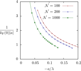
Figure 3: Inverse interaction strength at the center of the trap as a function of scattering length, for $\Omega=0$ and different number densities of particles $\mathcal{N}$.

To get an idea of the scales in a typical experiment, we can use that in Ref. Zwierlein05 a Fermi gas made out of ${}^{6}\mathrm{Li}$ atoms was studied in a trapping potential with radial frequency $\omega/(2\pi)=57\;\mathrm{Hz}$. This situation corresponds to $\lambda\sim 5.4\;\mu\mathrm{m}$ and $\hbar\omega/k_{B}\sim 2.7\;\mathrm{nK}$.

We will now first give a detailed overview of the results at zero rotation frequency. After that we will discuss the effects of rotating the trap and present the main objective of this work, the critical rotation frequency for vortex formation.

VII.1 Zero rotation frequency

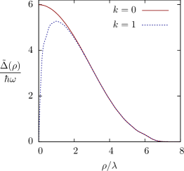
Figure 4: Pairing field as a function of radius, for $a=-0.1\lambda$, $\mathcal{N}=1000$ and $\Omega=0$.

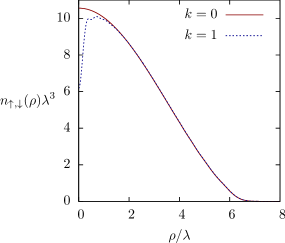
Figure 5: Number density as a function of radius, for $a=-0.1\lambda$, $\mathcal{N}=1000$ and $\Omega=0$.

In Fig. 4 we compare the pairing field of the vortex-free superfluid ($k=0$) with the pairing field of the vortex with unit angular momentum ($k=1$). These pairing fields were computed for $\mathcal{N}=1000$ and $a=-0.1\lambda$ with $N=64$. Because the data points lie so close to each other, we have only displayed a line that interpolates through the data points for visibility reasons. Since the rotation frequency was taken to be zero, the vortex is metastable.

The pairing field clearly vanishes at the center of the vortex. Away from the vortex core the pairing field is restored to its value in the $k=0$ case. The typical distance at which this happens is the BCS coherence length $\xi$. This implies that the size of the vortex core grows when decreasing the strength of the interaction. For very weak interactions, $\xi$ can become larger than the radius of the gas. In that case even a metastable vortex is no longer possible. In the second part of this section we will study the size of the vortex core at the critical rotation frequency for vortex formation in some detail.

The vortex also leaves its imprint on the corresponding density profiles which are displayed in Fig. 5. As already found in Refs. Bulgac03 ; Feder04 , the density at the center of the trap is significantly depleted in the presence of a vortex. To compensate for the removal of particles at the center, the gas will expand. This is a tiny effect and is, therefore, not visible in Fig. 5. In the next subsection we will study density depletion at the critical rotation frequency.

The density profile for normal pairing is very well described by the Thomas-Fermi approximation, which is the solution of Eq. (87). The pairing field however only agrees qualitatively with the Tomas-Fermi approximation, Eq. (89), as was also concluded in Ref. Bruun99 .

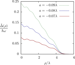
Figure 6: Pairing field as a function of radius, for $\mathcal{N}=100$, $k=0$ and different scattering lengths.

We have displayed pairing field profiles for $\mathcal{N}=100$ in Fig. 6. The interaction strength was taken to be weak, in the range $0.07\leq|a|/\lambda\leq 0.09$, which leads to small pairing fields. In such situations we encountered oscillations in the pairing field. To ensure that this is not a numerical artifact, we have compared these profiles computed with $N=32$, $N=48$ and $N=64$. We find that they are completely consistent with each other. The oscillations in the pairing field are only prominent in the case of a small number of particles with weak interactions.

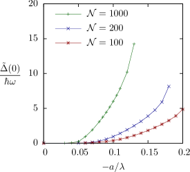
Figure 7: Pairing field at the center of the trap, as function of the scattering length, for different number of particles and $\Omega=0$.

Let us now study the effect of variation of the scattering length and the number of particles in the zero rotation limit. In Fig. 7 we display the pairing field at the center of the trap as a function of the scattering length. Clearly, increasing the interaction strength and the number of particles (i.e. the Fermi wave number) both lead to larger pairing fields. This is qualitatively in agreement with the BCS pairing formula, Eq. (89).

In Fig. 8 we have displayed the corresponding number density at the center of the trap. Increasing the number of particles leads naturally to a larger number density at the center. Stronger attractive interactions lead to a more compressed gas, which likewise results in a larger density at the center.

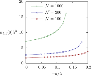
Figure 8: Density at the center of the trap, as function of the scattering length, for different number of particles, and $\Omega=0$.

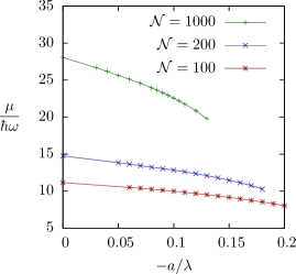
Figure 9: Chemical potential as function of the scattering length, for different number of particles, and $\Omega=0$.

In Fig. 9 we have displayed the corresponding chemical potential. Obviously a larger number of particles implies a larger chemical potential. The chemical potential decreases with increasing the strength of the interaction. This is because the Hartree term $-gn_{\downarrow,\uparrow}(\rho)$, which acts as a sort of inhomogeneous chemical potential, grows with increasing the interaction strength.

The radius of the gas can, to very good approximation, be obtained by inserting the values of the chemical potential in the Thomas-Fermi estimate, Eq. (88). This gives at zero rotation frequency $R/\lambda=\sqrt{2\mu/\hbar\omega}$. It then follows from Fig. 9 that increasing the number of particles increases the radius. On the other hand, increasing the interaction strength reduces the radius. The gas becomes more compressed because the interaction between the two components is attractive.

VII.2 Non-zero rotation frequency

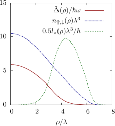
Figure 10: Pairing field, number density, and angular momentum density as a function of radius. The results correspond to a vortex-free superfluid with $\mathcal{N}=1000$, $a=-0.1\lambda$, and $\Omega=0.15\omega$.

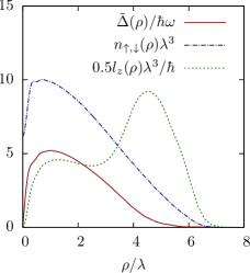
Figure 11: Same as in Fig. 10, but for a vortex with $k=1$.

To illustrate the effects of rotation, we have displayed the pairing field, the number density and the angular momentum density for $\Omega=0.15\omega$, $\mathcal{N}=1000$, and $a=-0.1\lambda$ in Fig. 10 ($k=0$) and Fig. 11 ($k=1$). These figures can be compared to the results at zero rotation frequency which are displayed in Figs. 4 and 5. As we will show below, $\Omega=0.15\omega$ is the critical rotation frequency for vortex formation in this situation.

A vortex-free superfluid state cannot carry angular momentum. For that reason the angular momentum density vanishes in the region where the pairing field is sizable, as can be seen in Fig. 10. Since angular momentum density appears at large $\rho$, it indicates the presence of unpaired fermions at the edges of the gas. Another way to observe this effect is that for large radial coordinates, the pairing field disappears before the number density does. It can be seen in Fig. 11 that a vortex generates angular momentum density in the superfluid region. For the same reasons as in the $k=0$ case, unpaired fermions are present at the boundaries of the gas.

By careful comparison of Figs. 10 and 11 one can observe that the pairing field of the vortex is slightly larger in the outer region. This is generally the case and leads in addition to the effects mentioned in the introduction to a fourth contribution to the energy difference between a vortex and a vortex-free phase. Rotation increases the radius of the cloud as well. However, at this rotation rate this is only a very small effect and is therefore not visible in the figures.

Now let us discuss the determination of the critical rotation frequencies for unpairing and vortex formation. To obtain these frequencies we have computed the Helmholtz free energy. The phase with the lowest free energy is the preferred phase.

In Fig. 12 we have displayed the Helmholtz free energy divided by the number of particles, for $\mathcal{N}=1000$ and $a=-0.1\lambda$. A number of interesting features of the superfluid are shown in this figure. First of all, the superfluid phase is always preferred over the unpaired phase, since $\Delta=0$ has the largest free energy. Furthermore, for $\Omega<0.05\omega$ the gas forms a vortex-free superfluid. It can be seen that in this region the free energy does not depend on the rotation frequency. This indicates that the entire gas is in a superfluid state. However, for $\Omega>0.05\omega$ the free energy of the vortex-free phase starts to decrease when increasing the rotation frequency. This implies that the gas has acquired angular momentum, which occurs via unpairing the fermions at the edges of the gas. Hence for $0.05\omega<\Omega<0.15\omega$ the gas forms a vortex-free superfluid with unpaired fermions at the boundaries. At $\Omega>0.15\omega$ a superfluid with a $k=1$ vortex becomes the preferred phase. One can see this more clearly in Fig. 13, where we have displayed the difference in free energy between the vortex phase with $k=1$ and the vortex-free phase. The critical rotation frequency can be found from interpolation of the data points which in this case yields $\Omega_{c}=0.149\omega$. For $\Omega<0.15\omega$ the $k=1$ phase is metastable. Because superfluids with a vortex carry angular momentum, the derivative of their free energy with respect to rotation frequency is negative, even at zero rotation frequency. In the unpaired phase this derivative vanishes at zero frequency, because the fully unpaired gas does not contain angular momentum at zero frequency.

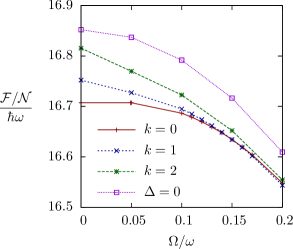
Figure 12: Helmholtz free energy divided by the number of particles, as a function of rotation frequency, for $a=-0.1\lambda$ and $\mathcal{N}=1000$. The label $k=0$ corresponds to a superfluid without vortices, the nonzero values of $k$ correspond to a single vortex at the center of the trap with angular momentum $k$. The label $\Delta=0$ corresponds to the situation in which all fermions are unpaired.

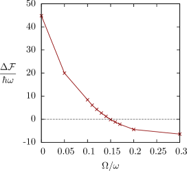
Figure 13: Difference in Helmholtz free energy per unit length in the $z$-direction between the vortex phase with $k=1$ and the vortex-free phase with $k=0$, as a function of rotation frequency, for $a=0.1\lambda$ and $\mathcal{N}=1000$.

At zero temperature, one can also compute the critical rotation frequency for unpairing in a more direct way. At zero rotation frequency all quasi-particle excitations (except the superfluid phonon) are gapped, i.e. $|E_{nmp_{z}}|>0$. As follows from the discussion in Appendix B, if $\mu_{\uparrow}=\mu_{\downarrow}$ and $\Omega=0$, both $E_{nmp_{z}}$ and $-E_{nmp_{z}}$ are eigenvalues of the Bogolibuov-de Gennes matrix. Rotation shifts these eigenvalues downwards by $m\hbar\Omega$. As long as no gapless mode arises the rotational contributions from positive and negative energies cancel so that this shift has no effect on the free energy. For that reason the free energy for $k=0$ stays constant up to a certain rotation frequency. Only when the first gapless mode appears, the free energy will change. The minimal rotation frequency at which this occurs is the critical rotation frequency for unpairing, $\Omega_{u}$. Thus this rotation frequency can be found from the solutions at $\Omega=0$ in the following way

$$\Omega_{u}=\mathrm{min}\left|\frac{1}{m\hbar}E_{nmp_{z}}(\Omega=0)\right|,$$ (91)

where the minimum is to be taken over all values of $n$, $m$, and $p_{z}$. Determination of $\Omega_{u}$ in this way is computationally much less expensive than obtaining it from the free energy.

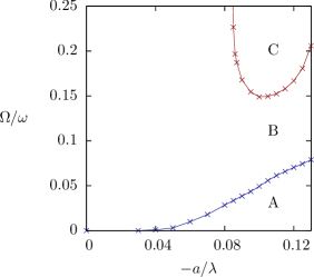
Figure 14: Phase diagram of a two-component Fermi gas as a function of scattering length and rotation frequency, for $\mathcal{N}=1000$ and $T=0$. The lines correspond to the phase boundaries. The label A indicates that the entire gas is in a vortex-free superfluid state. The label B indicates a vortex-free superfluid in the center with unpaired fermions in the outer regions of the gas. The label C indicates a superfluid with vortices in the center and unpaired fermions in the outer regions.

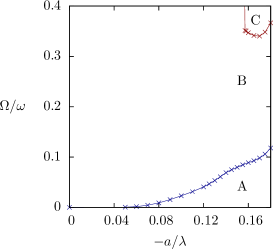
Figure 15: Same as in Fig. 14, but for $\mathcal{N}=200$.

Let us now discuss our main result: the phase diagram as a function of scattering length and rotation frequency. In Figs. 14 and 15 we have displayed these diagrams for $\mathcal{N}=1000$ and $\mathcal{N}=200$ respectively.

There are two transitions in these phase diagrams. The lower line denotes the unpairing transition. The order parameter corresponding to this transition is the angular momentum. This transition is of second order since the angular momentum changes continuously. At $T\neq 0$ this transition turns into a crossover. Hence at $\Omega=\Omega_{u}$ and $T=0$ the gas resides at a so-called quantum critical point. Above this critical point the order parameter behaves as $\mathcal{L}_{z}\sim t^{\beta}$ where $t=(\Omega-\Omega_{u})/\Omega_{u}$. We find numerically that the critical exponent has the value $\beta=1$.

The upper line denotes the critical rotation frequency for the formation of a vortex with unit angular momentum at the center of the trap. Energy arguments suggest that with increasing rotation frequency the first vortex configuration that will nucleate is a single vortex with $k=1$. A single vortex with $k>1$ will have lager energy, as can be seen in Fig. 12. Several vortices with $k=1$ have again larger energy and their nucleation would require larger than critical rotation frequencies. Therefore, the upper line shows the critical rotation frequency for vortex formation. The order parameter corresponding to this transition is the winding number of the vortex. Since this winding number changes discontinuously, this transition is of first order.

Increasing the absolute value of the scattering length leads to a larger critical rotation frequency for unpairing. Furthermore, for a given scattering length $\Omega_{u}$ becomes larger when the number of particles is increased. Both effects can be explained by the fact that a stronger bound pair is more difficult to break.

As can be seen from the phase diagrams, we find that vortices are formed only for relatively large negative scattering lengths. The critical rotation frequency for vortex formation has a minimum at a certain intermediate value of the scattering length. This minimum arises from the interplay of two effects. Firstly, the energy cost of creating a vortex at zero rotation frequency increases with increasing the negative scattering length. This explains the rise of the critical frequency at large negative scattering lengths. The second effect is caused by the difference in energy gain due to rotation. The $k=1$ phase will always have a larger rotational energy gain than the $k=0$ phase due to the angular momentum generated by the vortex. However, for small interaction strengths above the unpairing transition, the difference between these gains is relatively small. This is because in this case it is relatively easy to break the pairs at the boundaries of the gas, which contribute to the rotational energy gain in both the $k=0$ and $k=1$ phase. As a result of this effect the critical frequency increases for small negative scattering lengths. For a certain small scattering length the difference in rotational energy gain cannot overcome the costs associated to the vortex. For this reason at small negative scattering lengths the vortex phase has an abrupt transition to a vortex-free phase. We see that below $a\approx-0.155\lambda$ for $\mathcal{N}=200$ and $a\approx-0.085\lambda$ for $\mathcal{N}=1000$ vortex formation does not occur at all the rotation frequencies displayed in the phase diagram.

Vortex formation sets in at a lower rotation rate when the number density of particles is increased from $\mathcal{N}=200$ to $\mathcal{N}=1000$. For the number of particles we have investigated we find that the vortices always appear together with unpaired fermions at the edges of the gas. One could speculate that for a larger number of particles $\Omega_{c}$ will be reduced so that a vortex phase will appear before unpairing at the edges could become possible. In other words, we anticipate that for a large number of particles the phase diagram might feature a direct phase transition from the A to the C phase without the intermediate B phase.

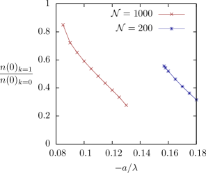
Figure 16: Relative density depletion at the core of a vortex, as a function of scattering length, at the critical rotation frequency for vortex formation.

In Fig. 16 we have displayed the central number density of a vortex over the central density of a vortex-free superfluid, at the transition to vortex formation. It can be seen that the amount of density depletion is relatively small for weak interactions and grows with increasing the interaction strength.

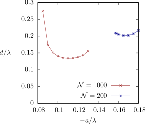
Figure 17: Half-width of the vortex as a function of scattering length, at the critical rotation frequency for vortex formation.

Let us define the half-width $d$ of the vortex to be the radius at which $\tilde{\Delta}(\rho)_{k=1}/\tilde{\Delta}(\rho)_{k=0}=1/2$. In Fig. 17 we have displayed this half-width at the transition for vortex-formation. For $\mathcal{N}=1000$ it can be clearly seen that weak interactions lead to larger vortices, which is caused by the increase of the BCS coherence length.

VIII Conclusions

In this article we studied a two-component Fermi gas with attractive $s$-wave interactions confined in a cylindrically symmetric harmonic trap. Our key results are summarized in a phase diagram spanned by the rotation frequency and scattering length for zero temperature and a fixed number of particles. Explicit results are shown for a number density of 1000 and 200 particles per unit harmonic oscillator length in the $z$-direction in Figs. 14 and 15 respectively.

To obtain the phase diagram we have used the two-particle irreducible effective action. We only took into account the leading order diagrams, which is equivalent to the Hartree-Fock-Bogoliubov approximation. This constrains our study to interaction strengths of magnitude $1/(k_{F}(0)|a|)\lesssim 1$. The equations we obtained were solved numerically using the DVR method based on Maxwell polynomials.

In the phase diagram three phases can be distinguished. For small rotation frequencies the entire gas forms a superfluid. At a certain critical frequency a second order transition occurs to a superfluid phase, which features unpaired fermions that are concentrated at the edges of the gas. At this critical rotation frequency the gas resides at a quantum critical point when the temperature vanishes. For even larger rotation frequencies vortices are formed via a first order transition. These vortices only appear for large negative scattering lengths. We have found that at a certain scattering length the critical rotation frequency for vortex formation has a minimum.

The presence of unpaired fermions at the boundaries of the gas results in an increase of the critical rotation frequency for vortex formation. For this reason one cannot use the free energy difference between a vortex phase and vortex-free phase at zero rotation frequency to compute the critical rotation frequency for vortex formation.

Our theoretical findings can be compared to the experiment at will, since the vortices have been observed in rotating two-component Fermi gases Zwierlein05 ; Zwierlein06 . It would be interesting to obtain the structure of the phase diagram from such experiments.

The theoretical understanding of the phase diagram can be improved in several ways. It would be worthwhile to investigate how the phase diagram is modified by temperature and by an imbalance in the number of fermions. Furthermore, it would be very useful to extend our analysis to larger interaction strengths, in order to obtain reliable results in the unitary regime.

Finally we would like to point out that vortices can also be induced by synthetic magnetic fields, as has been shown experimentally in a Bose-Einstein condensate Lin09 . Since such synthetic magnetic field is similar to rotation, another interesting extension of our work would be to compute the critical synthetic magnetic field strength for vortex formation in a two-component Fermi gas.

Appendix A The 2PI effective action

Consider an action $S=-\hbar\Psi^{\dagger}G_{0}^{-1}\Psi+S_{\mathrm{int}}$, where $G_{0}^{-1}$ denotes the bare inverse propagator and $S_{\mathrm{int}}$ is the part of the action that contains interactions. The partition function $Z[K]$ corresponding to this action in the presence of a source term $K$ is given by

$$Z[K]=\int\mathcal{D}\Psi^{\dagger}\mathcal{D}\Psi\exp\left[-S/\hbar+\ \Psi^{\dagger}K\Psi\right].$$ (92)

Let us denote the exact propagator in the presence of a source term $K$ as $G$. The 2PI effective action is defined as 2PI

$$\Gamma[G]=-\log Z[K]+\mathrm{Tr}(KG),$$ (93)

where $K$ has to be chosen in such a way that exact propagator in the presence of $K$ equals $G$. Since the exact propagator has to satisfy the Dyson-Schwinger equation, we can conclude that $K=G^{-1}-G_{0}^{-1}+\Sigma[G]$, where $\Sigma[G]$ is the 1PI self-energy. Taking the derivative of Eq. (93) with respect to $G$ gives $\frac{\delta\Gamma[G]}{\delta G}=K$, so that in the extremal points $\Gamma[G]=-\log Z[0]$. Inserting the expression for $K$ in Eq. (93) gives

$$\Gamma[G]=-\log Z_{2}-\mathrm{Tr}\left(G_{0}^{-1}G-1\right)+\mathrm{Tr}(\Sigma[G]G),$$ (94)

where $Z_{2}=Z[G^{-1}-G_{0}^{-1}+\Sigma[G]]$, which implies that $Z_{2}$ is the partition function of a theory with action $S_{2}=-\hbar\Psi^{\dagger}G^{-1}\Psi+S_{2,\mathrm{int}}$, where $S_{2,\mathrm{int}}=-\hbar\Psi^{\dagger}\Sigma[G]\Psi+S_{\mathrm{int}}$. One can now compute $-\log Z_{2}$ in a perturbative series, using $G$ as the propagator. It follows that the first two terms in this perturbative series are

$$-\log Z_{2}=-\mathrm{Tr}\log G^{-1}-\mathrm{Tr}\left(\Sigma[G]G\right)+\ldots.$$ (95)

Because the 1PI self-energy is now included in the interaction term, cancellations will occur such that only the 2PI diagrams survive 2PI . Hence

$$\Gamma[G]=-\mathrm{Tr}\log G^{-1}-\mathrm{Tr}\left(G_{0}^{-1}G-1\right)+\Gamma_{2}[G],$$ (96)

where $\Gamma_{2}[G]$ is now the sum of all 2PI diagrams generated by the interaction $S_{\mathrm{int}}$ with propagator $G$.

Appendix B Derivation of the Bogoliubov-de Gennes-equation

The inverse of a non-singular Hermitian matrix $A$ can be obtained from its eigenvalues $\lambda_{n}$ and the corresponding orthonormal eigenvectors $|n\rangle$, with $\langle n|m\rangle=\delta_{nm}$. Putting the $n$-th eigenvector in the $n$-th column of a new matrix $U$, one finds that $U$ is unitary, i.e. $U^{\dagger}U=1$ and $A=U\Lambda U^{\dagger}$, where $\Lambda=\mathrm{diag}(\lambda_{1},\lambda_{2},\ldots)$. The inverse of $A$ can now be constructed as $A^{-1}=U\Lambda^{-1}U^{\dagger}$, where $\Lambda^{-1}=\mathrm{diag}(1/\lambda_{1},1/\lambda_{2},\ldots)$. By performing the matrix multiplications, the last equation can be conveniently written as $A^{-1}=\sum_{n}|n\rangle\langle n|/\lambda_{n}$. A single component of the inverse matrix now reads $A^{-1}_{ij}=\sum_{n}\langle i|n\rangle\langle n|j\rangle/\lambda_{n}$.

The inverse Nambu-Gor’kov propagator $G^{-1}$, Eq. (33), can be written as $-\hbar G^{-1}=\hbar\partial/\partial\tau+\mathcal{H}$, where the Hermitian matrix $\mathcal{H}$ is given by Eq. (34).

Since $\mathcal{H}$ is independent of $\tau$, the eigenfunctions of $G^{-1}$ are a product of eigenfunctions of $\hbar\partial/\partial\tau$ and eigenfunctions of $\mathcal{H}$. Because $G(X,X^{\prime})$ has to satisfy anti-periodic boundary conditions in imaginary time, the properly normalized eigenfunctions of $\hbar\partial/\partial\tau$ are plane waves $\phi_{m}(\tau)=\exp(-\mathrm{i}\omega_{m}\tau)/\sqrt{\hbar\beta}$ with eigenvalue $-\mathrm{i}\hbar\omega_{m}$, where the Matsubara frequency $\omega_{m}=(2m+1)\pi/(\hbar\beta)$, with $m\in\mathbb{Z}$. Let us denote the normalized eigenfunctions of $\mathcal{H}$ as $\left(u_{i}(\boldsymbol{x}),v_{i}(\boldsymbol{x})\right)^{T}$ with corresponding eigenvalue $E_{i}$ (which is real). This eigenvalue equation which is given explicitly in Eq. (35) is known as the Bogoliubov-de Gennes equation Gennes64 . Normalization ($U^{\dagger}U=1$) implies that

$$\int\mathrm{d}^{3}x\,\left[|u_{i}(\boldsymbol{x})|^{2}+|v_{i}(\boldsymbol{x})|^{2}\right]=1.$$ (97)

Furthermore from completeness ($UU^{\dagger}=1$) one finds

$$\sum_{i}\left(\begin{array}[]{cc}u_{i}(\boldsymbol{x})u_{i}^{*}(\boldsymbol{x}^{\prime})&u_{i}(\boldsymbol{x})v_{i}^{*}(\boldsymbol{x}^{\prime})\\ v_{i}(\boldsymbol{x})u_{i}^{*}(\boldsymbol{x}^{\prime})&v_{i}(\boldsymbol{x})v_{i}^{*}(\boldsymbol{x}^{\prime})\end{array}\right)=\\ \delta(\boldsymbol{x}-\boldsymbol{x}^{\prime})\left(\begin{array}[]{cc}1&0\\ 0&1\end{array}\right).$$ (98)

We can now invert the inverse propagator $G^{-1}$, to obtain the Nambu-Gor’kov propagator,

$$G(X,X^{\prime})=-\frac{1}{\beta}\sum_{i}\sum_{m\in\mathbb{Z}}\frac{1}{-\mathrm{i}\hbar\omega_{m}+E_{i}}\mathrm{e}^{-\mathrm{i}\omega_{m}(\tau-\tau^{\prime})}\\ \times\left(\begin{array}[]{cc}u_{i}(\boldsymbol{x})u_{i}^{*}(\boldsymbol{x}^{\prime})&u_{i}(\boldsymbol{x})v_{i}^{*}(\boldsymbol{x}^{\prime})\\ v_{i}(\boldsymbol{x})u_{i}^{*}(\boldsymbol{x}^{\prime})&v_{i}(\boldsymbol{x})v_{i}^{*}(\boldsymbol{x}^{\prime})\end{array}\right).$$ (99)

We can see from this equation explicitly that $G_{\downarrow\uparrow}(X,X^{\prime})=G_{\uparrow\downarrow}(X^{\prime},X)^{*}$. In order to obtain the pairing field and the number densities we need to evaluate $G(X,X^{\prime}_{\pm})$. Here $X^{\prime}_{\pm}=(\boldsymbol{x},\tau\pm\eta)$ with $\eta$ an infinitesimal small positive number. In this limit one can compute the sum over Matsubara frequencies exactly. After using the completeness relation, Eq. (98), one then finds

$$G(X,X^{\prime}_{\pm}) = \sum_{i}f(E_{i})\left(\begin{array}[]{cc}u_{i}(\boldsymbol{x})u_{i}^{*}(\boldsymbol{x}^{\prime})&u_{i}(\boldsymbol{x})v_{i}^{*}(\boldsymbol{x}^{\prime})\\ v_{i}(\boldsymbol{x})u_{i}^{*}(\boldsymbol{x}^{\prime})&v_{i}(\boldsymbol{x})v_{i}^{*}(\boldsymbol{x}^{\prime})\end{array}\right)$$ (105)

$$-\theta(\mp)\delta(\boldsymbol{x}-\boldsymbol{x}^{\prime})\left(\begin{array}[]{cc}1&0\\ 0&1\end{array}\right),$$

where $f(E)=[\exp(\beta E)+1]^{-1}$ denotes the Fermi-Dirac distribution function and $\theta(x)$ is the unit-step function. The term proportional to the step function reflects the anti-commutation relation of the fermionic operators. The sum over $i$ runs over all eigenvalues. Using Eqs. (23), (25), and (26) one can now read off the expressions for the pairing field and the number densities.

If $\mu_{\uparrow}=\mu_{\downarrow}$, then the densities of the two species are equal so that $n_{\uparrow}(\boldsymbol{x})=n_{\downarrow}(\boldsymbol{x})$. By taking the complex conjugate of Eq. (35) it follows in this case that if $E_{i}$ is an eigenvalue of $\mathcal{H}$ with eigenvector $\left(u_{i}(\boldsymbol{x}),v_{i}(\boldsymbol{x})\right)^{T}$, then also $-E_{i}$ is an eigenvalue of $\mathcal{H}$ with eigenvector $\left(v^{*}_{i}(\boldsymbol{x}),-u^{*}_{i}(\boldsymbol{x})\right)^{T}$. One can now use this fact to restrict the sum over $n$ to eigenvectors with positive eigenvalues only, so that if $\mu_{\uparrow}=\mu_{\downarrow}$ one has

$$G(X,X^{\prime}_{\pm})=\sum_{E_{i}\geq 0}f(E_{i})\left(\begin{array}[]{cc}u_{i}(\boldsymbol{x})u_{i}^{*}(\boldsymbol{x}^{\prime})&u_{i}(\boldsymbol{x})v_{i}^{*}(\boldsymbol{x}^{\prime})\\ v_{i}(\boldsymbol{x})u_{i}^{*}(\boldsymbol{x}^{\prime})&v_{i}(\boldsymbol{x})v_{i}^{*}(\boldsymbol{x}^{\prime})\end{array}\right)\\ +\sum_{E_{i}\geq 0}[1-f(E_{i})]\left(\begin{array}[]{cc}v^{*}_{i}(\boldsymbol{x})v_{i}(\boldsymbol{x}^{\prime})&-v_{i}^{*}(\boldsymbol{x})u_{i}(\boldsymbol{x}^{\prime})\\ -u^{*}_{i}(\boldsymbol{x})v_{i}(\boldsymbol{x}^{\prime})&u_{i}^{*}(\boldsymbol{x})u_{i}(\boldsymbol{x}^{\prime})\end{array}\right)\\ -\theta(\mp)\delta(\boldsymbol{x}-\boldsymbol{x}^{\prime})\left(\begin{array}[]{cc}1&0\\ 0&1\end{array}\right).$$ (106)

From this equation one can read off the expressions for the number density and pairing field as they often appear in the literature. In this paper however we will solely use Eq. (105), because it leads to more compact expressions and has broader validity. The only slight disadvantage is that in Eq. (105) we have to sum over all eigenvalues.

To evaluate the grand potential, Eq. (30), we need to compute $\mathrm{Tr}\log G^{-1}$. Using that the trace of a logarithm is the sum over the logarithm of the eigenvalues one finds

$$\frac{1}{\beta}\mathrm{Tr}\log G^{-1}=\frac{1}{\beta}\sum_{i}\sum_{m\in\mathbb{Z}}\log(-\mathrm{i}\hbar\omega_{m}+E_{i}).$$ (107)

In order to perform the sum over the Matsubara frequencies one adds and subtracts the following infinite constant to the last equation

$$C=\frac{1}{\beta}\sum_{i}\left[\sum_{m\in\mathbb{Z}}\log(-\mathrm{i}\hbar\omega_{m})-\log(2)\right].$$ (108)

After summing over Matsubara frequencies one finds

$$\frac{1}{\beta}\mathrm{Tr}\log G^{-1}=\sum_{i}\left[\frac{|E_{i}|}{2}+\frac{1}{\beta}\log\left(1+\mathrm{e}^{-\beta|E_{i}|}\right)\right]+C.$$ (109)

Since $C$ is independent of $E_{i}$ it shifts the thermodynamic potential by an irrelevant constant and can therefore be ignored. Now the result Eq. (109) is not entirely correct. For example it is still infinite and in the limit of $\Delta(\boldsymbol{x})=0$ the grand potential of an unpaired Fermi gas is not obtained. To cure this problem one needs to take carefully the limit $\eta\rightarrow 0$. We proceed as in Refs. Stoof ; Negele88 to obtain

$$\frac{1}{\beta}\mathrm{Tr}\log G^{-1} = \sum_{i}\left[\frac{|E_{i}|}{2}+\frac{1}{\beta}\log\left(1+\mathrm{e}^{-\beta|E_{i}|}\right)\right]$$ (110)

$$-\sum_{i}\epsilon_{i},$$

here $\epsilon_{i}$ are the eigenvalues of the Hartree-Fock Hamiltonian, which is defined in Eq. (41). The last equation is indeed finite and reduces to the grand potential of an unpaired Fermi gas in the case $\Delta(\boldsymbol{x})=0$.

Appendix C Computation of nodes and weights of Maxwell polynomials

Any set of orthonormal polynomials of increasing degree $i$ and hence also the Maxwell polynomials $\phi_{i}(x)$ satisfies the following recursion relation (see e.g. Refs. Szego39 ; Gautschi04 ),

$$\sqrt{\beta_{i+1}}\phi_{i+1}(x)=(x-\alpha_{i})\phi_{i}(x)-\sqrt{\beta_{i}}\phi_{i-1}(x).$$ (111)

Here $\alpha_{i}$ and $\beta_{i}$ are the recursion coefficients.

Once the recursion coefficients are known, the nodes (which are the roots of $\phi_{N}(x)$) and weights of order $N$ can be found by solving the following eigenvalue equation numerically (see e.g. Refs. Szego39 ; Gautschi04 ),

$$\left(\begin{array}[]{cccc}\alpha_{0}&\sqrt{\beta_{1}}&&\\ \sqrt{\beta_{1}}&\alpha_{1}&\sqrt{\beta_{2}}&\\ &\ddots&\ddots&\ddots\\ &&\sqrt{\beta_{N-1}}&\alpha_{N-1}\\ \end{array}\right)\left(\begin{array}[]{c}\phi_{0}(x_{n})\\ \phi_{1}(x_{n})\\ \vdots\\ \phi_{N-1}(x_{n})\\ \end{array}\right)\\ =x_{n}\left(\begin{array}[]{c}\phi_{0}(x_{n})\\ \phi_{1}(x_{n})\\ \vdots\\ \phi_{N-1}(x_{n})\\ \end{array}\right).$$ (112)

The eigenvalues of the last equation are the $N$ nodes $x_{n}$. The weights follow directly from the eigenvectors in the following way (see e.g. Refs. Szego39 ; Gautschi04 ),

$$w_{n}=\left[\sum_{i=0}^{N-1}\phi_{i}(x_{n})^{2}\right]^{-1}.$$ (113)

The eigenvectors have to be normalized in such a way that that the orthonormality condition is satisfied, so that $\phi_{0}(x_{n})=[\int_{0}^{\infty}\mathrm{d}x\,w(x)]^{-1/2}$.

The recursion coefficients can be computed using the Stieltjes procedure, see e.g. Ref. Gautschi82 . Although the recursion coefficients for the Maxwell polynomials can be computed analytically in this way, this is impractical since the coefficients quickly become extremely complicated. Hence we have computed the recursion coefficients numerically. When doing so, one encounters another problem. The Stieltjes algorithm is extremely-ill conditioned Gautschi82 , implying that small errors blow up quickly. To avoid this, we followed Ref. Shizgal81 , and performed the Stieltjes algorithm using arbitrary precision arithmetic. This can be done using for example the computer program Mathematica. In order to compute all recursion coefficients up to $N=128$ with $22$ digits accuracy (so that it fits in double precision) we had to use 10,000 digits precision in the Stieltjes procedure.

In this way we have computed the weights and nodes of the Gauss-Maxwell quadrature with $p=1$ up to $N=128$. For $N=2,4,8$ and $16$ we could compare with tables presented in Ref. Shizgal81 . We find excellent agreement, almost up to machine precision accuracy.

Appendix D Computation of $\bar{H}$

Here we will compute $\bar{H}$, which is defined in Eq. (61). The integration over the parts of $H_{m}(\Omega)$ that are independent of $\rho$ is straightforward so that we can write

$$\begin{split}\left(\bar{H}\right)_{ij}&=\frac{1}{2}\hbar\omega\left[-(A)_{ij}+m^{2}(B)_{ij}\right]\\ &\quad-\hbar\Omega m\delta_{ij}+\frac{p_{z}^{2}}{2M}\delta_{ij},\end{split}$$ (114)

where the matrices $A$ and $B$ read

$$(A)_{ij} = \left(\lambda^{2}\frac{\mathrm{d}^{2}}{\mathrm{d}\rho^{2}}+\lambda^{2}\frac{1}{4\rho^{2}}-\frac{\rho^{2}}{\lambda^{2}}\right)_{ij},$$ (115)

$$(B)_{ij} = \left(\frac{\lambda^{2}}{\rho^{2}+\eta^{2}\lambda^{2}}\right)_{ij}.$$ (116)

First we will compute the matrix $(A)_{ij}$. We find

$$\begin{split}(A)_{ij}&=\int_{0}^{\infty}\mathrm{d}x\,w^{1/2}(x)l_{i}(x)\\ &\quad\quad\quad\times\left[\frac{\mathrm{d}^{2}}{\mathrm{d}x^{2}}+\frac{1}{4x^{2}}-x^{2}\right]w^{1/2}(x)l_{j}(x)\\ &=\int_{0}^{\infty}\mathrm{d}x\,w(x)l_{i}(x)\\ &\quad\quad\quad\times\left[\frac{\mathrm{d}^{2}}{\mathrm{d}x^{2}}+\left(\frac{1}{x}-2x\right)\frac{\mathrm{d}}{\mathrm{d}x}-2\right]l_{j}(x).\end{split}$$ (117)

To obtain the last line we have used that $w(x)=x\exp(-x^{2})$. Eq. (117) can be rewritten as

$$(A)_{ij} = \int_{0}^{\infty}\mathrm{d}x\,w(x)l_{i}(x)\left[\frac{\mathrm{d}^{2}}{\mathrm{d}x^{2}}-2x\frac{\mathrm{d}}{\mathrm{d}x}-2\right]l_{j}(x)$$ (118)

$$+\int_{0}^{\infty}\mathrm{d}x\,w(x)l_{i}(x)\frac{1}{x}\left[\frac{\mathrm{d}}{\mathrm{d}x}l_{j}(x)-l_{j}^{\prime}(0)\right]$$

$$+\,l_{j}^{\prime}(0)\int_{0}^{\infty}\mathrm{d}x\,w(x)\frac{1}{x}\left[l_{i}(x)-l_{i}(0)\right]$$

$$+\,l_{i}(0)l_{j}^{\prime}(0)\int_{0}^{\infty}\mathrm{d}x\,\exp(-x^{2}).$$

This form has the advantage that the integrands of the first three terms are products of the weight function $w(x)$ and a polynomial of degree less than $2N$. Hence we can evaluate these terms exactly using the Gauss-Maxwell quadrature. The last term of Eq. (118) can also be computed analytically and is equal to $\l_{i}(0)l_{j}^{\prime}(0)\sqrt{\pi}/2$.

To proceed we will first evaluate the first and second order derivatives of $l_{j}(x)$ at the nodes $x_{i}$ which become (see also Ref. Szalay93 )

$$\begin{split}\left.\frac{\mathrm{d}}{\mathrm{d}x}l_{j}(x)\right|_{x=x_{i}}&=\frac{1}{\sqrt{w_{i}}}\xi_{i}\delta_{ij}\\ &\quad+\frac{1}{\sqrt{w_{i}}}\frac{C_{i}}{C_{j}}\frac{1}{x_{i}-x_{j}}(1-\delta_{ij}),\end{split}$$ (119)

$$\left.\frac{\mathrm{d}^{2}}{\mathrm{d}x^{2}}l_{j}(x)\right|_{x=x_{i}}=\frac{1}{\sqrt{w_{i}}}\left(\xi_{i}^{2}-\zeta_{i}\right)\delta_{ij}\\ +\frac{1}{\sqrt{w_{i}}}\frac{C_{i}}{C_{j}}\left[\frac{2\xi_{i}}{x_{i}-x_{j}}-\frac{2}{(x_{i}-x_{j})^{2}}\right](1-\delta_{ij}),$$ (120)

where

$$\xi_{i} = \sum_{n=1,n\neq i}^{N}\frac{1}{x_{i}-x_{n}},$$ (121)

$$\zeta_{i} = \sum_{n=1,n\neq i}^{N}\frac{1}{(x_{i}-x_{n})^{2}},$$ (122)

$$C_{i} = \sqrt{w_{i}}{\prod_{n=1,n\neq i}^{N}(x_{i}-x_{n})}.$$ (123)

Furthermore $l_{i}(0)$ and $l_{j}^{\prime}(0)$ are given by

$$l_{i}(0) = \frac{1}{\sqrt{w_{i}}}\prod_{n=1,n\neq i}^{N}\frac{x_{n}}{x_{n}-x_{i}},$$ (124)

$$l_{j}^{\prime}(0) = -D_{j}l_{j}(0),$$ (125)

$$D_{j} = \sum_{n=1,n\neq j}^{N}\frac{1}{x_{n}}.$$ (126)

Putting everything together we find that

$$\begin{split}(A)_{ij}&=\left[\xi_{i}^{2}-\zeta_{i}+\left(\frac{1}{x_{i}}-2x_{i}\right)\xi_{i}-2\right]\delta_{ij}\\ &\quad+\frac{C_{i}}{C_{j}}\left[\frac{2\xi_{i}}{x_{i}-x_{j}}-\frac{2}{(x_{i}-x_{j})^{2}}\right.\\ &\quad\quad\quad\quad+\left.\left(\frac{1}{x_{i}}-2x_{i}\right)\frac{1}{x_{i}-x_{j}}\right](1-\delta_{ij})\\ &\quad+D_{j}\left[\sum_{n=1}^{N}\frac{w_{n}}{x_{n}}-\frac{1}{2}\sqrt{\pi}\right]l_{i}(0)l_{j}(0).\end{split}$$ (127)

The matrix $A$ is symmetric as follows from Eq. (117), although this is not directly clear from the last equation.

Now let us compute the matrix $(B)_{ij}$. Expressed in terms of an integral over the basis functions this matrix reads

$$(B)_{ij}=\int_{0}^{\infty}\mathrm{d}x\,w(x)l_{i}(x)l_{j}(x)\frac{1}{x^{2}+\eta^{2}}.$$ (128)

We are interested in $(B)_{ij}$ in the limit of small $\eta$. Therefore in the rest of the calculations, we will drop terms that are of order $\eta$ and higher. Like in the calculation for $(A)_{ij}$ we rewrite the integrand in such a way that we get terms which are a polynomial of degree less than $2N$ times $w(x)$. We can then easily integrate these terms using the Gauss-Maxwell quadrature. We can rewrite $(B)_{ij}$ in the limit $\eta\rightarrow 0$ as

$$\begin{split}(B)_{ij}&=\int_{0}^{\infty}\mathrm{d}x\,w(x)\left[l_{i}(x)-l_{i}(0)\right]\left[l_{j}(x)-l_{j}(0)\right]\frac{1}{x^{2}}\\ &\quad+l_{i}(0)\int_{0}^{\infty}\mathrm{d}x\,w(x)\left[l_{j}(x)-l_{j}(0)-xl_{j}^{\prime}(0)\right]\frac{1}{x^{2}}\\ &\quad+l_{j}(0)\int_{0}^{\infty}\mathrm{d}x\,w(x)\left[l_{i}(x)-l_{i}(0)-xl_{i}^{\prime}(0)\right]\frac{1}{x^{2}}\\ &\quad+\left[l_{i}(0)l_{j}^{\prime}(0)+l^{\prime}_{i}(0)l_{j}(0)\right]\int_{0}^{\infty}\mathrm{d}x\,\exp(-x^{2})\\ &\quad+l_{i}(0)l_{j}(0)\int_{0}^{\infty}\mathrm{d}x\,\frac{x}{x^{2}+\eta^{2}}\exp(-x^{2}).\end{split}$$ (129)

The first three terms of the last equation can be computed using the Gauss-Maxwell quadrature. The next term can be evaluated analytically. The last integral can be computed analytically for small $\eta$. We obtain

$$(B)_{ij}=\frac{1}{x_{i}^{2}}\delta_{ij}-\left[\frac{1}{2}\gamma_{E}+\log(\eta)+\sum_{n=1}^{N}\frac{w_{n}}{x_{n}^{2}}\right.\\ \left.+(D_{i}+D_{j})\left(\frac{1}{2}\sqrt{\pi}-\sum_{n=1}^{N}\frac{w_{n}}{x_{n}}\right)\right]l_{i}(0)l_{j}(0),$$ (130)

where $\gamma_{E}$ denotes the Euler-Mascheroni constant.

The last equation shows that $(B)_{ij}$ has a logarithmic singularity for $\eta=0$. For that reason we had to regularize the centrifugal potential in Eq. (55). An alternative way of treating such singularity in the DVR method is discussed in Ref. Vincke93 .

References

- (1) M. W. Zwierlein, J. R. Abo-Shaeer, A. Schirotzek, C. H. Schunck, and W. Ketterle, Nature 435, 1047 (2005).
- (2) M. W. Zwierlein, A. Schirotzek, C. H. Schunck, and W. Ketterle, Science 311, 492 (2006).
- (3) M. W. Zwierlein, C. H. Schunck, A. Schirotzek, and W. Ketterle, Nature 442, 54 (2006).
- (4) C. H. Schunck, M. W. Zwierlein, A. Schirotzek, and W. Ketterle, Phys. Rev. Lett. 98, 050404 (2007).
- (5) H. T. C. Stoof, M. Houbiers, C. A. Sackett, and R. G. Hulet, Phys. Rev. Lett. 76, 10 (1996).
- (6) M. Houbiers, R. Ferwerda, H. T. C. Stoof, W. I. McAlexander, C. A. Sackett, and R. G. Hulet, Phys. Rev. A 56, 4864 (1997).
- (7) B. Clancy, L. Luo, and J.E. Thomas, Phys. Rev. Lett. 99, 140401 (2007); S. Riedl, E. R. Sánchez Guajardo, C. Kohstall, J. Hecker Denschlag, and R. Grimm, New J. Phys. 13, 035003 (2011).
- (8) S. Giorgini, L. P. Pitaevskii, and S. Stringari, Rev. Mod. Phys. 80, 1215 (2008).
- (9) M. Rodriguez, G.-S. Paraoanu, and P. Törmä, Phys. Rev. Lett. 87, 100402 (2001).
- (10) N. Nygaard, G. M. Bruun, C. W. Clark, and D. L. Feder, Phys. Rev. Lett. 90, 210402 (2003).
- (11) A. Bulgac and Y. Yu, Phys. Rev. Lett. 91, 190404 (2003).
- (12) D. L. Feder, Phys. Rev. Lett. 93, 200406 (2004).
- (13) M. Takahashi, T. Mizushima, M. Ichioka, and K. Machida, Phys. Rev. Lett. 97, 180407 (2006).
- (14) M. Iskin, Phys. Rev. A 78, 021604(R) (2008).
- (15) A. Bulgac, Y. L. Luo, P. Magierski, K. J. Roche, and Y. Yu, Science 332, 1288 (2011).
- (16) S. S. Botelho and C. A. R. Sá de Melo, Phys. Rev. Lett. 96, 040404 (2006).
- (17) G. Tonini, F. Werner, and Y. Castin, Eur. Phys. J. D 39, 283 (2008).
- (18) H. Zhai and T.L. Ho, Phys. Rev. Lett. 97, 180414 (2006).
- (19) M. Y. Veillette, D. E. Sheehy, L. Radzihovsky, and V. Gurarie, Phys. Rev. Lett. 97, 250401 (2006).
- (20) G. Möller and N. R. Cooper, Phys. Rev. Lett. 99, 190409 (2007).
- (21) Y.-P. Shim, R. A. Duine, and A. H. MacDonald, Phys. Rev. A 74, 053602 (2006).
- (22) M. L. Kulic, A. Sedrakian, and D. H. Rischke, Phys. Rev. A 80, 043610 (2009).
- (23) G. M. Bruun and L. Viverit, Phys. Rev. A 64, 063606 (2001).
- (24) N. Nygaard, G. M. Bruun, B. I. Schneider, C. W. Clark, and D. L. Feder, Phys. Rev. A 69, 053622 (2004).
- (25) J. Bardeen, R. Kümmel, A. E. Jacobs, and L. Tewordt, Phys. Rev. 187, 556 (1969).
- (26) I. Bausmerth, A. Recati, and S. Stringari, Phys. Rev. Lett. 100, 070401 (2008).
- (27) M. Urban and P. Schuck, Phys. Rev. A 78, 011601(R) (2008).
- (28) M. Iskin and E. Tiesinga, Phys. Rev. A 79, 053621 (2009).
- (29) M. R. Matthews, B. P. Anderson, P. C. Haljan, D. S. Hall, C. E. Wieman, and E. A. Cornell, Phys. Rev. Lett. 83, 2498 (1999); K. W. Madison, F. Chevy, W. Wohlleben, and J. Dalibard, Phys. Rev. Lett. 84, 806 (2000); J. R. Abo-Shaeer, C. Raman, J. M. Vogels, and W. Ketterle, Science 292, 476 (2001).
- (30) A. L. Fetter, Rev. Mod. Phys. 81, 647 (2009).
- (31) S. Stringari, Phys. Rev. Lett. 82, 4371 (1999).
- (32) Y. Kawaguchi and T. Ohmi, arXiv:cond-mat/0411018.
- (33) R. Sensarma, M. Randeria, and T. L. Ho, Phys. Rev. Lett. 96, 090403 (2006).
- (34) C.-C. Chien, Y. He, Q. Chen, and K. Levin, Phys. Rev. A 73, 041603(R) (2006).
- (35) H. T. C. Stoof, K. B. Gubbels, and D. B. M. Dickerscheid, Ultracold Quantum Fields (Springer 2009).
- (36) G. Bruun, Y. Castin, R. Dum, and K. Burnett, Eur. Phys. J. D 7, 433 (1999).
- (37) K. Huang and C. N. Yang, Phys. Rev. 105, 767 (1957).
- (38) J. M. Cornwall, R. Jackiw, and E. Tomboulis, Phys. Rev. D 10, 2428 (1974).
- (39) J. M. Luttinger and J. C. Ward, Phys. Rev. 118, 1417 (1960).
- (40) R. Haussmann, W. Rantner, S. Cerrito, and W. Zwerger, Phys. Rev. A 75, 023610 (2007).
- (41) H. Abuki, Prog. Theor. Phys. 110, 937 (2003); D. H. Rischke, Prog. Part. Nucl. Phys. 52, 197 (2004); S. B. Ruester and D. H. Rischke, Phys. Rev. D69, 045011 (2004).
- (42) P. G. de Gennes, Superconductivity of metals and alloys (W.A. Benjamin, New York, 1964).
- (43) A. Bulgac and Y. Yu, Phys. Rev. Lett. 88, 042504 (2002).
- (44) M. Grasso and M. Urban, Phys. Rev. A 68, 033610 (2003).
- (45) B. Shizgal, J. Comp. Phys. 41, 309 (1981).
- (46) J. C. Light, I. P. Hamilton, and J. V. Lill, J. Chem. Phys. 82, 1400 (1985).
- (47) D. Baye and P. H. Heenen, J. Phys. A. 19, 2041 (1986).
- (48) V. Szalay, J. Chem. Phys. 99, 1978 (1993).
- (49) D. Baye, M. Hesse, and M. Vincke, Phys. Rev. E 65, 026701 (2002).
- (50) D. Baye and M. Vincke, Phys. Rev. E 59, 7195 (1999).
- (51) Y.-J. Lin, R. L. Compton, K. Jiménez-García, J. V. Porto, and I. B. Spielman, Nature 462, 628 (2009).
- (52) J. W. Negele and H. Orland, Quantum many-particle systems (Westview Press 1988).
- (53) G. Szegö, Orthogonal Polynomials (American Mathematical Society 1939).
- (54) W. Gautschi, Orthogonal Polynomials: computation and approximation (Oxford University Press 2004).
- (55) W. Gautschi, SIAM J. Sci. Stat. Comput. 3, 289 (1982).
- (56) C. G. Broyden, Math. Comp. 19, 577 (1965).
- (57) M. Vincke, L. Malegat, and D. Baye, J. Phys. B. 26, 811 (1993).