The energy analysis for the monte carlo simulations of a diffusive shock

Abstract

According to the shock jump conditions, the total fluid’s mass, momentum, and energy should be conserved in the entire simulation box. We perform the dynamical Monte Carlo simulations with the multiple scattering law for energy analysis. The various energy functions of time are obtained by monitoring the total particles’ mass, momentum, and energy in the simulation box. In conclusion, the energy analysis indicates that the smaller energy losses in the prescribed scattering law are, the harder the energy spectrum produced is.

1 Introduction

The gradual solar energetic particles with a power-law energy spectrum are generally thought to be accelerated by the first-Fermi acceleration mechanism at the interplanetary shocks (IPs) (Axford et al., 1977; Krymsky, 1977; Bell, 1978; Blandford & Ostriker, 1978). It is well known that the diffusive shock accelerated the particles efficiently by the accelerated particles scattering off the instability of Alfven waves which are generated by the accelerated particles themselves (Gosling et. al. , 1981; Cane et.al. , 1990; Lee & Ryan, 1986; Berezhko, et.al. , 2003; Pelletier, et.al., 2006). The diffusive shock acceleration (DSA) is so efficient that the back-reaction of the accelerated particles on the shock dynamics cannot be neglected. So the theoretical challenge is how to efficiently model the full shock dynamics (Berezhko & Völk , 2006; Caprioli, et. al., 2010; Zank, 2000; Li et al., 2003; Lee, 2005). To efficiently model the shock dynamics and the particles’ acceleration, there are largely three basic approaches: stationary Monte Carlo simulations, fully numerical simulations, and semi-analytic solutions. In the stationary Monte Carlo simulations, the full particle population with a prescribed scattering law is calculated based on the particle-in-cell (PIC) techniques (Ellison et al., 1996; Vladimirov et al., 2006). In the fully numerical simulations, a time-dependent diffusion-convection equation for the CR transport is solved with coupled gas dynamics conservation laws (Kang & Jones, 2007; Zirakashvili & Aharonian, 2010). In the semi-analytic approach, the stationary or quasi-stationary diffusion-convection equations coupled to the gas dynamical equations are solved (Blasi, et. al., 2007; Malkov, et. al., 2000). Since the velocity distribution of suprathermal particles in the Maxwellian tail is not isotropic in the shock frame, the diffusion-convection equation cannot directly follow the injection from the non-diffusive thermal pool into the diffusive CR population. So considering both the quasi-stationary analytic models and the time-dependent numerical models, the injection of particles into the acceleration mechanism is based on an assumption of the transparency function for thermal leakage (Blasi, et. al., 2005; Kang & Jones, 2007; Vainio & Laitinen, 2007). Thus, the dynamical Monte Carlo simulations based on the PIC techniques are expected to model the shock dynamics time-dependently and also can eliminate the suspicion arising from the assumption of the injection (Knerr, Jokipii & Ellison, 1996; Wang & Yan, 2011). In plasma simulation (PIC and hybrid), there is no distinction between thermal and non-thermal particles, hence particle injection is intrinsically defined by the prescribed scattering properties, and so it is not controlled with a free parameter (Caprioli, et. al., 2010).

Actually, Wang et al. Wang & Yan (2011) have extended the dynamical Monte Carlo models with an anisotropic scattering law. Unlike the previous isotropic prescribed scattering law, the Gaussian scattering angular distribution is used as the complete prescribed scattering law. According to the extended prescribed scattering law, we obtained a series of similar energy spectrums with little difference in terms of the power-law tail. However, it is not clear how such a prescribed scattering law can affect the particles’ diffusion and the shock dynamics evolution. To probe these problems, we expect to diagnose the energy losses in the simulations by monitoring all of the behaviors of the simulated particles.

In the time-dependent Monte Carlo models coupled with a Gaussian angular scattering law, the results show that the total energy spectral index and the compression ratio are both effected by the prescribed scattering law. Specifically, the total energy spectral index is an increasing function of the dispersion of the scattering angular distribution, but the subshock’s energy spectral index is a digressive function of the dispersion of the scattering angular distribution (Wang & Yan, 2011). In the dynamical Monte Carlo simulations, one find that it is the only way for the particles to escape upstream via free escaped boundary (FEB). With the same size of the FEB which limited the maximum energy of accelerated particles, we find that different Gaussian scattering angular distribution generate different maximum energy particles through the scattering process at the same simulation time.

In an effort to verify the efficiency of the energy transfer from the thermal to superthermal and the effect of the shock dynamics evolution on the shock structures, we perform a dynamical Monte Carlo code on Matlab with Gaussian scattering angular distribution by monitoring the particles’ mass, momentum and energy as functions of time. Our Gaussian scattering angular distribution algorithm consists of four cases involving four specific standard deviation values. This aim is to know if the various particle’s loss functions are dependent on the prescribed scattering law and the various kinds of losses can directly determine the total compression ratio and final energy spectral index with the same timescale of the shock evolutions and the same size of FEB.

In Section 2, the basic simulation method is introduced with respect to the Gaussian scattering angular distributions for monitoring the particles’ mass, momentum and energy as function of time in each case. In Section 3, we present the shock simulation results and the energy analysis for all cases with four assumptions of scattering angle distributions. Section 4 includes a summary and the conclusions.

2 Method

The Monte Carlo model is a general model, although it is considerably expensive computationally, and it is important in many applications to include the dynamical effects of nonlinear DSA in simulations. Since the prescribed scattering law in Monte Carlo model instead of the field calculation in hybrid simulations (Giacalone, 2004; Winske & Omidi, 2011), we assume that particle scatters elastically according to a Gaussian distribution in the local plasma frame and that the mean free path (mfp) is proportional to the gyroradius (i.e., $\lambda\propto r_{g}$), where $r_{g}=pc/(qB)$, and its value is proportional to its momentum. Under the prescribed scattering law, the injection is correlated with those “thermal” particles which manage to diffuse the shock front for obtaining additional energy gains and become superthermal particles (Ellison et al., 2005).

However, the basic theoretical limit to the accelerated particle’s energy arises from the accelerated particle’s Larmor radius, which must be smaller than the dimensions of the acceleration region by at least $v_{s}/c$ (Hillas, 1984), where $v_{s}$ is the shock velocity. The limitation to the maximum energy of accelerated particles due to the large Larmor radius would be ameliorated if the scattering angular distribution is varied. In these simulations, the size of the FEB is set as a finite length scale matched with the maximum diffusive length scale. Here, we further investigate the possibility that the accelerated particles scatter off the background magnetic field in the acceleration region with not only an isotropic scattering angular distribution, but also with an anisotropic scattering angular distribution. Actually, this anisotropic distribution would probably produce an important effect on simulation results. With the same size of FEB, the scattering law applied isotropic distribution or anisotropic distribution would produce different maximum energy particles. So an anisotropic scattering law in the theory of the CR-diffusion is also needed (Bell, 2004).

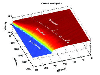
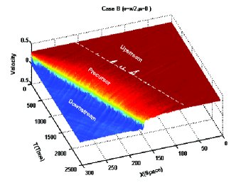
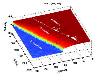
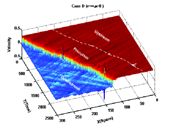
Figure 1: The entire evolutional velocity profiles in four cases. The dashed line denotes the FEB position in each plot. The precursor is located in the area between the downstream region and the upstream region in each case.

The particle-in-cell techniques are applied in these dynamical Monte Carlo simulations. The simulation box is divided up into some number of cells and the field momentum is calculated at the center of each cell (Forslund, 1985; Spitkovsky, 2003; Nishikawa, et. al., 2008). The total size of a one-dimensional simulation box is set as $X_{max}$ and it is divided into the number of grids $N_{max}$. Upstream bulk speed $U_{0}$ with an initial Maxwellian thermal velocity $V_{L}$ in their local frame and the inflow in a “pre-inflow box” (PIB) are both moving along one-dimensional simulation box. The parallel magnetic field $B_{0}$ is along the $\hat{x}$ axis direction in the simulation box. A free escaped boundary (FEB) with a finite size in front of the shock position is used to decouple the escaped particles from the system as long as the accelerated particles beyond the position of the FEB. The simulation box is a dynamical mixture of three regions: upstream, precursor and downstream. The bulk fluid speed in upstream is $U=U_{0}$, the bulk fluid speed in downstream is $U=0$, and the bulk fluid speed with a gradient of velocity in the precursor region is $U_{0}>U>0$. Because of the prescribed scattering law instead of the particle’s movement in the fields, the injected particles from the thermalized downstream into the precursor for diffusive processes are controlled by the free elastic scatter mechanism. To obtain the information of the total particles in different regions at any time, we build a database for recording the velocities, positions, and time of the all particles, as well as the index and the bulk speeds of the grids. The scattering angle distributions are presented by Gaussian distribution function with a standard deviation $\sigma$, and an average value $\mu$ involving four cases: (1) Case A: $\sigma=\pi$/4, $\mu=0$. (2) Case B: $\sigma=\pi$/2, $\mu=0$. (3) Case C: $\sigma=\pi$, $\mu=0$. (4) Case D: $\sigma=\infty$, $\mu=0$. These presented simulations are all based on a one-dimensional simulation box and the specific parameters are based on Wang & Yan (2011).

3 Results & analysis

We present the entire shock evolution with the velocity profiles of the time sequences in each case as shown in Figure 1. The total velocity profiles are divided into three parts with respect to the shock front and the FEB locations. The upstream bulk speed $U_{0}$ dynamically slows down by passing though the precursor region, and its value decreases to zero in the downstream region (i.e. $U_{d}=0$). The precursor explicitly shows a different slope of the bulk velocity and different final FEB locations in different cases. The present velocity profiles are similar to the density profiles in the previous simulations by Wang & Yan (2011), and the different prescribed scattering law leads to the different shock structures.

Table 1: The Calculated Results

Items	Case A	Case B	Case C	Case D
$M_{loss}$	1037	338	182	127
$P_{loss}$	0.0352	0.0189	0.0123	0.0084
$E_{loss}$	0.7468	0.5861	0.4397	0.3014
$E_{feb}$	0.8393	0.5881	0.5310	0.5022
$E_{in}$	1.5861	1.1742	0.9707	0.8036
$E_{tot}$	3.3534	3.4056	3.3574	3.4026
$R_{in}$	38.25%	25.67%	19.98%	14.80%
$R_{loss}$	22.27%	17.21%	13.10%	8.86%
$r_{tot}$	8.1642	6.3532	5.6753	5.0909
$r_{sub}$	2.0975	3.0234	3.1998	3.9444
$\Gamma_{tot}$	0.7094	0.7802	0.8208	0.8667
$\Gamma_{sub}$	1.8668	1.2413	1.1819	1.0094
$v_{sh}$	-0.0419	-0.0560	-0.0642	-0.0733
$v_{sub}$	0.0805	0.1484	0.1613	0.2159
$V_{Lmax}$	11.4115	14.2978	17.2347	20.5286
$E_{peak}$	0.1650keV	0.1723keV	0.1986keV	0.2870keV
$E_{max}$	1.23MeV	1.93MeV	2.80MeV	4.01MeV

The units of mass, momentum, and energy are normal to the proton mass $m_{p}$, initial momentum $P_{0}$, and initial energy $E_{0}$, respectively. The last two rows are shown as scaled values.

The various losses of the particles and the calculated results of the shocks at the end of the simulation for the four cases are listed in Table 1. The initial box energy is $E_{0}$. The subshock’s compression ratio $r_{sub}$ and the total compression ratio $r_{tot}$ are calculated from the fine velocity structures in the shock frame in each case, respectively. The total energy spectral index $\Gamma_{tot}$ and the subshock’s energy spectral index $\Gamma_{sub}$ are deduced from the corresponding total compression ratio $r_{tot}$ and the subshock’s compression ratio $r_{sub}$ in each case. The $M_{loss}$, $P_{loss}$ and $E_{loss}$ are the mass, momentum, and energy losses which are produced by the escaped particles via the FEB, respectively.

We have monitored the mass, momentum and energy of the total particles in each time step in each case. Figure 2 shows all the types of energy functions with respect to time. The total energy $E_{tot}$ is the energy summation over the time in the entire simulation box at any instant in time. The box energy $E_{box}$ presents the actual energy in the simulation box at any instant in time. The supplement energy $E_{PIB}$ is the summation of the amount of energy from the pre-inflow box (at the left boundary of the simulation box) which enters into the simulation box with a constant flux. The $E_{feb}$ presents a summation of the amount of energy held in the precursor region. The $E_{out}$ indicates a summation of the amount of energy which escapes via the FEB. Clearly, the total energy in the simulation at any instant in time is not equal to the actual energy in the box at any instant in time in each plot.

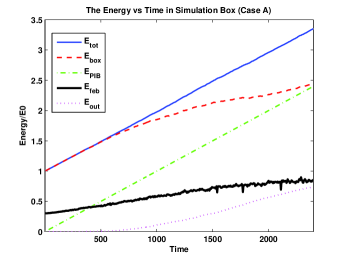
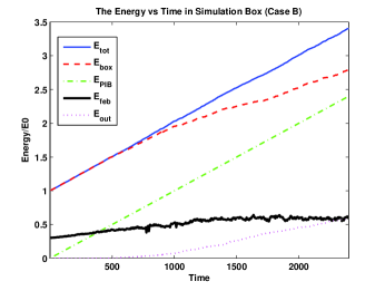
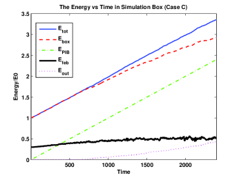
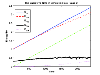
Figure 2: Various energy values vs. time (all normalized to the initial total energy $E_{0}$ in the simulation box) in each case. All quantities are calculated in the box frame.

It can be shown that the incoming particles (upstream) decrease their energy (as viewed in the box frame) as they scatter in the shock precursor region. If each incoming particle loses a small amount of energy as it first encounters the shock, this would produce a constant linear divergence between the curves for $E_{box}$ and $E_{tot}$. Actually, the cases in these simulations produce the non-linear divergence between the curves for $E_{box}$ and $E_{tot}$, consistent with Figure 2. Such behavior is evident from individual particle’s trajectories. Physically, all the kinds of the losses occur in the precursor region owing to the “back reaction” of the accelerated ions and the escaped particles via FEB. Various energy functions obviously show that the case applying the anisotropic scattering law produces a higher energy loss, while the case applying the isotropic scattering law produces a lower energy loss. Consequently, we consider that the prescribed scattering law dominate the energy losses.

3.1 Energy losses

With monitoring each particle in the grid of the simulation box in any increment of the time, the escaped particles’ mass, momentum, and energy loss functions with the time are obtained and shown in Figure 3. Among these energy functions, the inverse flow function is obtained from the injected particles from the thermalized downstream to the precursor.

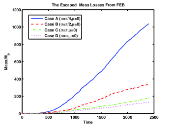
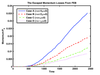
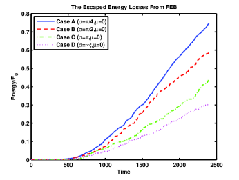
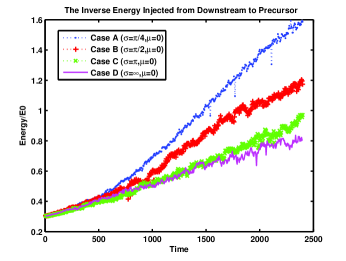
Figure 3: The four plots denote the mass losses, momentum losses, energy losses and the inverse energy, respectively. The solid line, dashed line, dash-dotted line and the dotted line represent the cases A, B, C and D in the first three plots. In the last plot, the dashed lines marked with the signal of dot, plus, and cross, and the solid line represent the cases A, B, C and D, respectively. The units are normal to the proton mass $M_{p}$, initial total momentum $P_{0}$ and initial total energy $E_{0}$, respectively.

Since the FEB is limited to be in front of the shock position with the same size in each case, once a single accelerated particle moves backward to the shock beyond the position of the FEB, we exclude this particle from the total system as the loss term in the mass, momentum, and the energy conservation equations. According to the Rankine-Hugoniot (RH) relationships, the compression ratio of the nonrelativistic shock with a large Mach number is not allowed to be larger than the standard value of four (Pelletier, 2001). Owing to the energy losses which inevitably exist in the simulations, the calculated results show a decreasing values of the loss of the mass, momentum, and the energy from the cases A, B, and C to D, respectively. Simultaneously, the inverse energy injected from downstream to precursor is also a decreasing values of $(E_{in})_{A}=1.5861$, $(E_{in})_{B}=1.1742$, $(E_{in})_{C}=0.9707$, and $(E_{in})_{D}=0.8036$ from the cases A, B, and C to D, respectively. The accurate energy losses are the values of $(E_{loss})_{A}=0.7468$, $(E_{loss})_{B}=0.5861$, $(E_{loss})_{C}=0.4397$, and $(E_{loss})_{D}=0.3041$ in each case. The inverse energy is the summation of the energy loss $E_{loss}$ and the net energy $E_{feb}$ in the precursor (i.e. $E_{in}=E_{loss}+E_{feb}$). So it is no wonder that the total shock ratios are all larger than four because of the existence of energy losses in all cases. Therefore, the difference of the energy losses and the inverse energy can directly affect all aspects of the simulation shocks.

3.2 Subshock structure

Figure 4 shows the subshock structure in each case at the end of the simulation time. The specific structure in each plot consists of three main parts: precursor, subshock and downstream. The smooth precursor with a larger scale is between the FEB and the subshock’s position $X_{sub}$, where the bulk velocity gradually decreases from the upstream bulk speed $U_{0}$ to $v_{sub1}$. And the size of the precursor is almost equal to the diffusive length of the maximum energy particle accelerated by the diffusion process. The sharp subshock with a shorter scale only spans three-grid-lengthsb involving a deep deflection of the bulk speed abruptly decreasing from $v_{sub1}$ to $v_{sub2}$, where the scale of the three-grid-length is largely equal to the mean free path of the averaged thermal particles in the thermalized downstream. The value of the subshock’s velocity can be defined by the difference value of the two boundaries of the subshock.

$$v_{sub}=|v_{sub1}-v_{sub2}|.$$ (1)

With the upstream bulk speed slowing down from $U_{0}$ to zero, the size of the downstream region is increasing with its constant shock velocity $v_{sh}$ in each case, and the bulk speed is $U=0$ owing to the dissipation processes which characterize the downstream. The gas subshock is just an ordinary discontinuous classical shock embedded in the total shock with a comparably larger scale (Berezhko & Ellison , 1999).

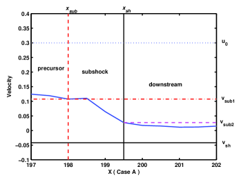
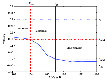
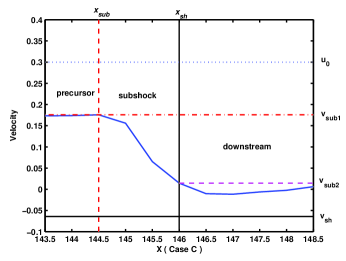
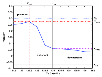
Figure 4: Final subshock fine structures in the four cases. The vertical solid and dashed lines indicate the positions of the shock front and subshock in each plot, respectively. The horizontal solid, dashed, dash-dotted and dotted lines show the values of the shock velocity $v_{sh}$, subshock velocity $v_{sub2}$, subshock velocity $v_{sub1}$ and initial bulk velocity $U_{0}$, respectively. Three vertical blocks in each plot represent the three deflections of velocity: precursor region, subshock region and downstream region. All values of the velocity are based on the box frame.

According to the subtle shock structures, the shock compression ratio can be cataloged into two classes: one class presents the entire shock named the total compression ratio $r_{tot}$ and the other class characterizes the subshock named the subshock’s compression ratio $r_{sub}$. The values of the two kinds of compression ratios can be reduced by the following formulas, respectively.

$$r_{tot}=u_{1}/u_{2},\\$$ (2)

$$r_{sub}=(v_{sub}+|v_{sh}|)/|v_{sh}|,$$ (3)

where $u_{1}=u_{0}+|v_{sh}|$ , $u_{2}=|v_{sh}|$, and $u_{1}(u_{2})$ is the upstream (downstream) velocity in the shock frame, $v_{sub}$ is the subshock’s velocity determined by Equation 1, and the shock velocity $v_{sh}$ at the end of the simulation is decided by the following:

$$v_{sh}=(X_{max}-X_{sh})/T_{max},$$ (4)

where $X_{max}$ is the total length of the simulation box, $T_{max}$ is the total simulation time, and $X_{sh}$ is the position of the shock at the end of the simulation. The specific calculated results are shown in Table 1. The values of the subshock’s compression ratios are $(r_{sub})_{A}$=2.0975 , $(r_{sub})_{B}$=3.0234, $(r_{sub})_{C}$=3.1998 and $(r_{sub})_{D}$=3.9444 corresponding to the cases A, B, C and D, respectively. The total shock compression ratios with the values of $(r_{tot})_{A}$=8.1642, $(r_{tot})_{B}$=6.3532, $(r_{tot})_{C}$=5.6753, and $(r_{tot})_{D}$=5.0909 also correspond to the cases A, B, C and D, respectively. In comparison, the total shock compression ratios are all larger than the standard value four and the subshock’s compression ratios are all lower than the standard value four. Additionally, the value of the total shock compression ratio decreases from Cases A, B, and C to D, while the subshock’s compression ratio increases from Cases A, B, and C to D. These differences are naturally attributed to the different fine subshock structures.

3.3 Maximum energy

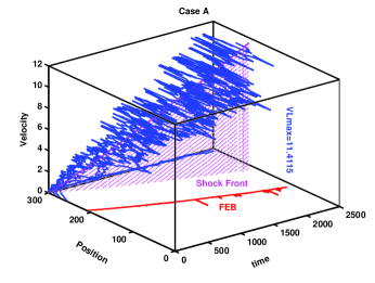
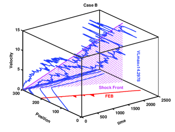
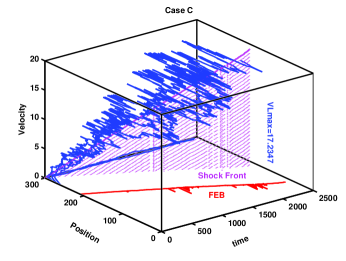
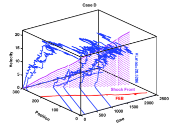
Figure 5: The individual particles with their thermal velocity in the local frame vs their positions with respect to time in each plot. The shaded area indicates the shock front, the solid line in the bottom plane denotes the position of the FEB in each case, respectively. Some irregular curves trace the individual particle’s trajectories near the shock front with time. The maximum energy of accelerated particles in each case is marked with the value of the velocity, respectively.

We select some individual particles from the phase-space-time database recording the all particles’ information. The trajectories of the selected particles are shown in Figure 5. One of these trajectories clearly shows the route of the maximum energy of accelerated particle which undergoes the multiple collisions with the shock front in each case. The maximum value of the energy is apparently different in each case with increasing values of $(VL_{max})_{A}=11.4115$, $(VL_{max})_{B}=14.2978$, $(VL_{max})_{C}=17.2347$, and $(VL_{max})_{D}=20.5286$ from the Cases A, B, and C to D, respectively. And those particles with a value higher than the cutoff energy are unavailable owing to their escaping from the FEB. The statistical data show the number of escaped particles in each case decreases with the number of particles $(n_{esc})_{A}=1037$, $(n_{esc})_{B}=338$, $(n_{esc})_{C}=182$, and $(n_{esc})_{D}=127$ from Cases A, B, and C to D, correspondingly. Except for the maximum energy of the particle in each case, the other particles show that some of them obtained finite energy accelerations from the multiple crossings with the shock and some of them do not have additional energy gains owing to their lack of probability for crossing back into the precursor due to their small diffusive length scale. The statistical data also exhibit that the inverse energy injected from the downstream back to upstream is characterized by a decreasing reflux rate of $(R_{in})_{A}=38.25\%$, $(R_{in})_{B}=25.67\%$, $(R_{in})_{C}=19.98\%$, and $(R_{in})_{D}=14.80\%$ in corresponding Cases A, B, C, and D. With the decrease of the inverse energy from Cases A, B, and C to D, the corresponding energy losses are also reduced at the rate of $(R_{loss})_{A}=22.27\%$, $(R_{loss})_{B}=17.21\%$, $(R_{loss})_{C}=13.10\%$, and $(R_{loss})_{D}=8.86\%$ in each case, respectively. Although the maximum energy of the accelerated particles should be identical because of the limitation of the same size of the FEB in four cases, the cutoff energy values are still modified by the existence of the energy losses in the different cases applied with the different prescribed Gaussian scattering laws.

3.4 Energy spectrum

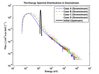
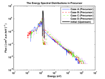
Figure 6: The two plots present the final energy spectrums on the downstream and the precursor region, respectively. The thick solid line with a narrow peak at $E=$1.3105keV in each plot represents the same initial Maxwell energy distributions in each case. The solid, dashed, dash-dotted and dotted extended curves with the “power-law” tail present the energy spectral distributions corresponding to Cases A, B, C and D, respectively. All these energy spectrum distributions are plotted in the same shock frame.

The energy spectrums with the “power-law” tail are calculated in the shock frame from the downstream region and the precursor region at the end of simulation, respectively. The same initial Maxwellian distribution in each case is shown in each plot in Figure 6. As shown in Figure 6, the calculated energy spectrums indicate that the four extended curves in the downstream region with an increasing value of the central energy peak $(E_{peak})_{A}=0.1650keV$, $(E_{peak})_{B}=0.1723keV$, $(E_{peak})_{C}=0.1986keV$, and $(E_{peak})_{D}=0.2870keV$ characterize the Maxwellian distributions in the ”heated-downstream” from Cases A ,B, and C to D, respectively. The value of the total energy spectral index $(\Gamma_{tot})_{A}=0.7094$, $(\Gamma_{tot})_{B}=0.7802$, $(\Gamma_{tot})_{C}=0.8208$, and $(\Gamma_{tot})_{D}=0.8667$ in each case indicates the Maxwellian distribution in the ”heated-downstream” with a decreasing deviation to the “power-law” distribution from Cases A, B, and C to D, correspondingly. But the value of the subshock’s energy spectral index $(\Gamma_{sub})_{A}=1.8668$, $(\Gamma_{sub})_{B}=1.2413$, $(\Gamma_{sub})_{C}=1.1819$, and $(\Gamma_{sub})_{D}=1.0094$ present the energy spectrum distribution with a “power-law” tail in each case implying there is an increasing rigidity of the spectrum from the Cases A, B, and C to D, respectively. The cutoff energy at the “power-law” tail in the energy spectrum is given with an increasing value of $(E_{max})_{A}$=1.23 MeV, $(E_{max})_{B}$=1.93 MeV, $(E_{max})_{C}$=2.80 MeV and $(E_{max})_{D}$=4.01 MeV from the Cases A, B, C and D, respectively. In the precursor region, the final energy spectrum is divided into two very different parts in each case. The part in the range from the low energy to the central peak shows an irregular fluctuation in each case. The irregular fluctuation indicates that the cold upstream fluid slows down and becomes the “thermal fluid” by the nonlinear “back reaction” processes. And the other part in the range beyond the central peak energy shows a smooth “power-law” tail in each case.

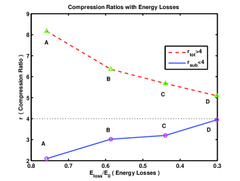
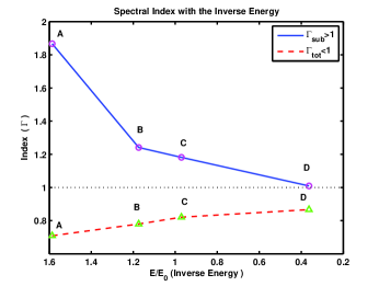
Figure 7: Two plots show the correlation of the compression ratio vs the energy losses and the correlation of the energy spectral index vs the inverse energy, respectively. The triangles represent the total compression ratios and the total energy spectral index of the all cases in each plot. The circles indicate the subshock’s compression ratios and the subshock’s energy spectral index of all cases in each plot.

As shown in Figure 7, the two kinds of shock compression ratios are both apparently dependent on the energy losses with respect to these four presented simulations. As viewed from Cases A, B, and C to D, the total compression ratio is a decreasing function of the energy losses and each value is larger than the standard value four, the subshock’s compression ratio is an increasing function of the energy losses and each value is lower than four. However, both the total compression ratio and the subshock’s compression ratio approximate the standard value of four as the energy loss decreases. According to the DSA theory, if the energy loss is limited to be the minimum, the simulation models based on the computer will more closely fit the realistic physical situation. Additionally, the energy spectral index is also fairly dependent on the inverse energy from the thermalized downstream region into the precursor region.

4 Summary and conclusions

In summary, we performed the dynamical Monte Carlo simulations using the Gaussian scattering angular distributions based on the Matlab platform by monitoring the particle’s mass, momentum and energy at any instant in time. The specific mass, momentum and energy loss functions with respect to time are presented. A series of analyses of the particle losses are obtained in the four cases. We successfully examine the relationship between the shock compression ratio and the energy losses, as well as verify the consistency of the energy spectral index with the inverse energy injected from the downstream to precursor region in the simulation cases which are applied with the prescribed Gaussian scattering angular distributions.

In conclusion, the relationship of the shock compression ratio with the energy losses via FEB verify that the energy spectral index is determined by the inverse energy function with time. In fact, these energy losses simultaneously depend on the assumption of the prescribed scattering law. As expected, the maximum energy of accelerated particles is limited by the size of the FEB according to the maximum mean free path in each case. However, there is still a fairly large difference between the maximum energy of the particle from the different cases with the same size of the FEB. We find that the total energy spectral index increases as the standard deviation value of the scattering angular distribution increases, but the subshock’s energy spectral index decreases as the standard deviation value of the scattering angular distribution increases. In these multiple scattering angular distribution simulations, the prescribed scattering law dominates the energy losses and the inverse energy. Consequently, the case of applying a prescribed law which leads to the minimum energy losses will produce a harder subshock’s energy spectrum than those in the cases with larger energy losses. These relationships will drive us to find a newly prescribed scattering law which leads to the minimum energy losses, making the shock compression ratio more closely approximate the standard value of four for a nonrelativistic shock with high Mach number in astrophysics.

References

- Axford et al. (1977) Axford, W.I., Leer, E., & Skadron, G., 1977 in Proc. 15th Int. Comsmic Ray Conf. (Plovdiv), 132
- Bell (1978) Bell, A. R., 1978, MNRAS, 182, 147.
- Bell (2004) Bell, A. R., 2004, MNRAS, 353, 550.
- Berezhko & Ellison (1999) Berezhko, E. G. & Ellison, D. C. 1999, Astrophys. J., 526, 385
- Berezhko, et.al. (2003) Berezhko, E. G., Ksenofontov, L. T. & Völk H. J. 2003, Astron. Astrophys., 412, L11.
- Berezhko & Völk (2006) Berezhko, E. G., & Völk H. J. 2006, Astron. Astrophys., 451, 981.
- Blandford & Ostriker (1978) Blandford, R. D., & Ostriker, J. ,P. 1978, Astrophys. J., 221, L29.
- Blasi, et. al. (2007) Blasi, P., Amato, E., & Caprioli, D., 2007, M.N.R.A.S., 375,1471
- Blasi, et. al. (2005) Blasi, P., Gabici, S., & Vannoni, G., 2005, M.N.R.A.S., 361,907
- Cane et.al. (1990) Cane, H. V., von Rosenvinge, T. T., & McGuire, R. E., 1990, J. Geophys. Res., 95, 6575.
- Caprioli, et. al. (2010) Caprioli, D., Kang, H., Vladimirov, A. E. & Jones, T. W., 2010, M.N.R.A.S., 407,1773
- Ellison et al. (1996) Ellison, D. C., Baring, M. G., & Jones, F. C. , 1996, Astrophys. J.473,1029
- Ellison, Möbius & Paschmann (1990) Ellison, D. C., Möbius, E. & Paschmann, G.1990, Astrophys. J., 352, 376
- Ellison et al. (2005) Ellison, D. C., Blasi & Gabici , 2005, in Proc. 29th Int. Comsmic Ray Conf. (India).
- Forslund (1985) Forslund, D. W. 1990, Space Sci. Rev., 42, 3
- Giacalone (2004) Giacalone, J. , 2004, Astron. Astrophys., 609, 452.
- Gosling et. al. (1981) Gosling, J.T., Asbridge, J.R., Bame, S.J., Feldman, W.C., Zwickl,R. D.,Paschmann, G.,Sckopke, N., & Hynds, R. J. 1981, J. Geophys. Res., 866, 547
- Hillas (1984) Hillas, 1984, ARA&A, 22, 425.
- Jones & Ellison (1991) Jones, F. C., & Ellison, D. C., 1991, Space Science Reviews, 58, 259.
- Kang & Jones (2007) Kang H. & Jones T.W. 2007, A. Ph., 28, 232
- Knerr, Jokipii & Ellison (1996) Knerr, J. M., Jokipii, J. R. & Ellison, D. C. 1996, Astrophys. J., 458, 641
- Krymsky (1977) Krymsky, G. F., 1977, Akad. Nauk SSSR Dokl., 243, 1306
- Lee & Ryan (1986) Lee, M. A., & Ryan, J. M., 1986, Astrophys. J., 303, 829
- Lee (2005) Lee, M. A., 2005, APJS, 158, 38
- Malkov, et. al. (2000) Malkov, M. A., Diamond, P. H., & Vlk, H. J., 2000, Astrophys. J. Lett., 533,171
- Nishikawa, et. al. (2008) Niemiec, J. , Pohl, M. , Stroman, T. , & Nishikawa, K.-I., 2008, Astrophys. J., 684, 1174.
- Li et al. (2003) Li, G., Zank, G. P., & Rice, W. K. M., 2003, JGR 108,1082
- Ostrowski (1988) Ostrowski, M. , 1988, M.N.R.A.S., 233, 257
- Pelletier (2001) Pelletier, G. 2001, Lecture Notes in Physics, , 576, 58
- Pelletier, et.al. (2006) Pelletier, G. , Lemoine, M. & Marcowith, A. , 2006, Astron. Astrophys., 453,181.
- Spitkovsky (2003) Spitkovsky, A. , 2008, Astrophys. J. Lett., 673, L39.
- Vainio & Laitinen (2007) Vainio, R., & Laitinen, T., 2007, Astrophys. J., 658, 622.
- Vladimirov et al. (2006) Vladimirov, A., Ellison, D. C., & Bykov, A., 2006, Astrophys. J., 652,1246
- Wang & Yan (2011) Wang, X., & Yan, Y., 2011, Astron. Astrophys., 530, A92.
- Winske & Omidi (2011) Winske, D. , & Omidi, N. , 1996, J. Geophys. Res., 101,17287–17304.
- Zank (2000) Zank, G., Rice, W.K.M., & Wu, C. C., 2000, JGR, 105, 25079
- Zirakashvili & Aharonian (2010) Zirakashvili, V. N. & Aharonian, F. A., 2010, Astrophys. J., 708, 965