On the Tradeoff Between Multiuser Diversity and Training Overhead in Multiple Access Channels

Abstract

We consider a single antenna narrowband multiple access channel in which users send training sequences to the base station and scheduling is performed based on minimum mean square error (MMSE) channel estimates. In such a system, there is an inherent tradeoff between training overhead and the amount of multiuser diversity achieved. We analyze a block fading channel with independent Rayleigh distributed channel gains, where the parameters to be optimized are the number of users considered for transmission in each block and the corresponding time and power spent on training by each user. We derive closed form expressions for the optimal parameters in terms $K$ and $L$, where $K$ is the number of users considered for transmission in each block and $L$ is the block length in symbols. Considering the behavior of the system as $L$ grows large, we optimize $K$ with respect to an approximate expression for the achievable rate, and obtain second order expressions for the resulting parameters in terms of $L$. The resulting number of users trained is shown to scale as $O(\frac{L}{(\log L)^{2}})$, and the corresponding achievable rate as $O(\log\log L)$.

I Introduction

Multiuser diversity is a powerful technique for taking advantage of channel fluctuations in wireless communication systems [1], [2], [3]. In a cell with a large number of users experiencing independent fading, high rates of communication can be obtained by scheduling only the users with the strongest channels. More specifically, in a multiple access channel (MAC) with an average total power constraint, symmetric fading statistics and full channel state information (CSI), ergodic sum capacity is maximized by allowing only the strongest user to transmit, with the power allocation given by waterfilling [1]. Furthermore, when the tail of the fading distribution satisfies certain conditions, the ergodic sum capacity scales as $\log\log K_{\mathrm{total}}$, where $K_{\mathrm{total}}$ is the total number of users in the system [2]. In particular, this result holds for channel distributions with exponential tails, such as the Rayleigh distribution.

In practical systems, full CSI is an unreasonable assumption, and channel estimates are instead obtained via training. This can require significant overhead in terms of both time and power, particularly when the number of users in the system is large. While there exists a large amount of literature on scheduling with training and limited feedback, most of it is for the broadcast channel (BC) rather than the MAC. In the BC, a common setup is for the base station to broadcast a training signal which allows each user to estimate their own channel, perform self-selection, and feed back information to the base station [4, 5]. If the system is time division duplex (TDD) then such techniques are also possible in the MAC, as are fully distributed approaches [6].

Motivated by the fact that many wireless systems are frequency division duplex (FDD), we consider the case that the uplink and downlink channels differ and the users do not know their own channels. In this case, training sequences are sent from the users to the base station rather than vice versa. Given a finite coherence time, there is a limit to how long can be spent on training before the channel estimates become stale, and hence a limit on how many users can train the base station during this time. Consequently, the ergodic sum capacity remains bounded as the total number of users in the system grows large, and $\log\log K_{\mathrm{total}}$ scaling is not achieved.

I-A Contributions and Previous Work

In this paper, we consider a narrowband single antenna MAC with block fading and independent Rayleigh distributed channel coefficients. The block length in symbols is denoted by $L$. During each block, $K$ users train the base station one at a time, after which the base station uses the channel estimates to perform scheduling. We aim to maximize a lower bound on the ergodic capacity with respect to the training time, training power and number of users considered for transmission.

Our approach is similar to [7], from which we borrow much of our notation. In [7], training time and power are optimized along with the number of subchannels trained in a single-user wideband system. This problem is one of choosing a number of parallel channels to train and transmit data over, whereas we consider the problem of training and user scheduling over a shared channel. While these problems bear some similarities, there are several key differences between the two. For example, in [7] an arbitrarily large number of subchannels can be trained simultaneously without interference, whereas in the MAC, interference can only be avoided using orthogonal training sequences, leading to a significant loss in the temporal degrees of freedom. Similarly, after training, our setup does not allow for multiple users to transmit their data in parallel.

A summary of our main contributions is as follows: (1) We derive exact expressions for the optimal proportion of both time and power spent on training in terms of $K$ and $L$. (2) By analyzing the behavior of the system as $K$ and $L$ grow large with $K=o(L)$, we obtain second order expressions for each of the parameters in terms of $K$ and $L$. (3) We optimize $K$ over an approximate expression for the achievable rate and obtain the resulting second order expressions for each of the parameters in terms of $L$, as well as the corresponding estimation error and achievable rate. Numerical results are used to show that these expressions approximate the optimal parameters well for finite values of $L$.

Other related work is presented in [8]–[13]. In [8], the work of [7] is extended to the multiuser wideband case with random training sequences, under the assumption that the number of users grows linearly with the block length. That is, optimization is done over the number of subchannels for a fixed number of users but not vice versa. Analysis of a multiuser narrowband system is performed in [9], but with a focus on the downlink channel. Specifically, the authors in [9] assume that each user can obtain perfect knowledge of their own channel, and that feedback to the base station requires a fixed number of bits per user. Optimization of training in a single-user MIMO system is presented in [10] and [11]. In [10] the focus is on one-way communication where a training sequence is followed immediately by the data, while in [11] the feedback of quantized CSI to the transmitter is considered. In [12], a multiuser FDD MIMO broadcast channel is studied, assuming zero-forcing beamforming with an equal number of users and base station antennas. This is extended to other settings in [13], including TDD and erroneous feedback.

I-B Paper Organization

The remainder of the paper is organized as follows. We present the system model and formulate the problem in Section II. We derive expressions for the optimal parameters in terms of $K$ and $L$ in Section III. In Section IV we derive asymptotic expressions for the parameters in terms of $L$ alone. A discussion of the asymptotic expressions is given in Section V. Numerical results are presented in Section VI, and conclusions are drawn in Section VII.

The following notations are used throughout the paper. $\log(\cdot)$ denotes the natural logarithm, and all rates are in units of nats per channel use. $\mathbb{E}[\cdot]$ denotes statistical expectation, and $\stackrel{{\scriptstyle d}}{{=}}$ means “distributed as”. The distribution of a circularly symmetric complex Gaussian (CSCG) vector with mean $\mathbf{\mu}$ and covariance matrix $\mathbf{\Sigma}$ is denoted by $\mathbb{CN}(\mathbf{\mu},\mathbf{\Sigma})$. $|\cdot|$ denotes magnitude, and $\|\cdot\|$ denotes Euclidean norm. $\mathbf{0}_{M\times 1}$ denotes an $M\times 1$ vector of zeros, and $\mathbf{I}_{M}$ denotes the $M\times M$ identity matrix. For two functions $f(L)$ and $g(L)$, we write $f=O(g)$ if $|f|\leq c|g|$ for some constant $c$ when $L$ is sufficiently large, $f=o(g)$ if $\lim_{L\rightarrow\infty}\frac{f}{g}=0$, $f=\Theta(g)$ if $f=O(g)$ and $f\neq o(g)$, and $f\sim g$ if $\lim_{L\rightarrow\infty}\frac{f}{g}=1$.

II System Model and Problem Statement

We consider a single antenna FDD narrowband MAC with $K_{\mathrm{total}}$ users communicating with a base station. The transmitted data is assumed to be delay-insensitive. The channel is modeled as a Rayleigh block fading channel with $L$ symbols per block and independent fades between blocks. Within each block, $K$ users are considered for transmission. We assume that $K_{\mathrm{total}}$ is sufficiently large so that any choice of $K$ is permitted, provided that the total training time does not exceed the block length. The group of users considered varies between blocks using a deterministic selection scheme known to both the base station and the users. For example, for fairness, the $K$ users could be chosen in a round robin fashion or using a synchronized pseudo-random number generator.

Under this setup, the system is described by

$$\mathbf{y}=\sum_{k=1}^{K}h_{k}\mathbf{x}_{k}+\mathbf{z}$$

where $\mathbf{y}$ is the $L\times 1$ received signal vector, $\mathbf{x}_{k}$ is the $L\times 1$ transmit symbol vector for user $k$, $h_{k}\stackrel{{\scriptstyle d}}{{=}}\mathbb{CN}(0,\sigma_{h}^{2})$ is the channel coefficient of user $k$, and $\mathbf{z}\stackrel{{\scriptstyle d}}{{=}}\mathbb{CN}(\mathbf{0}_{L\times 1},\sigma_{z}^{2}\mathbf{I}_{L})$ is an $L\times 1$ vector of CSCG noise samples. The transmitted symbols are subject to an average total power constraint,

$$\mathbb{E}\left[\frac{1}{L}\sum_{k=1}^{K}\|\mathbf{x}_{k}\|^{2}\right]\leq P.$$ (1)

The users are assumed to be synchronized with their coherence blocks aligned in time, and each user is assumed to experience independent fading. We note that due to the symmetry of the setup, the power constraint could be replaced by a more realistic individual average power constraint of $\frac{P}{K_{\mathrm{total}}}$ for each of the $K_{\mathrm{total}}$ users without affecting the analysis. However, we do not consider the asymmetric case, which would require the consideration of issues such as fairness.

Since the channel coefficients $h_{k}$ are unknown at the base station, the start of each coherence block is dedicated to training. One at a time, the $K$ users under consideration transmit training sequences, each having an equal length denoted by $\overline{T}$. The total number of symbols during training is denoted by $T=K\overline{T}$. Each user transmits with power $P_{T}$ when sending their own training sequence, and remains silent while the other training sequences are sent. At the base station, a minimum mean square error (MMSE) channel estimate $\widehat{h}_{k}$ is obtained for each user, with the corresponding channel estimation error denoted by $e_{k}=h_{k}-\widehat{h}_{k}$. The variance of this error is given by [7]

$$\sigma_{e}^{2}=\mathbb{E}\left[|e_{k}|^{2}\right]=\sigma_{h}^{2}-\sigma_{\widehat{h}}^{2}=\sigma_{h}^{2}\left(1-\frac{\sigma_{h}^{2}\overline{T}P_{T}}{\sigma_{h}^{2}\overline{T}P_{T}+\sigma_{z}^{2}}\right)$$ (2)

where $\sigma_{\widehat{h}}^{2}=\mathbb{E}[|\widehat{h}_{k}|^{2}]$ is the variance of $\widehat{h}_{k}$. This variance is the same for all users, since each user is assumed to use the same amount of time and power for training.

Since the ergodic sum capacity of a fading channel with MMSE estimation is not yet known, we instead use a lower bound achieved by treating the channel estimation error as additive Gaussian noise. In a general setup where multiple users may be scheduled with various powers, this achievable rate is given by [14]

$$\underline{C}=(1-\alpha)\mathbb{E}\left[\log\left(1+\frac{\sum_{k\in\mathcal{K}}P_{D,k}|\widehat{h}_{k}|^{2}}{\sigma_{e}^{2}\sum_{k\in\mathcal{K}}P_{D,k}+\sigma_{z}^{2}}\right)\right]$$ (3)

where $\alpha=\frac{T}{L}$ is the fraction of the coherence time dedicated to training, $\mathcal{K}$ is the set of users scheduled to transmit, and $P_{D,k}$ is the transmit power of user $k$ during data transmission. While the cardinality of $\mathcal{K}$ may in general be a function of the channel estimates, it is evident from (3) that for any given total power $\sum_{k\in\mathcal{K}}P_{D,k}>0$ the term inside the expectation in (3) is maximized by allowing only the user with the strongest $|\widehat{h}_{k}|^{2}$ to transmit. We therefore restrict our attention to the case that $|\mathcal{K}|=1$ and the base station schedules the user with the strongest channel estimate, $\max_{k=1,...,K}|\widehat{h}_{k}|^{2}$, which will be denoted as $|\widehat{h}^{*}|^{2}$. We assume that the feedback from the base station is error-free and takes up an insignificant fraction of the coherence time, and hence the selected user has $L-T$ symbols available for data transmission. Under this scheme, the achievable rate is given by

$$\underline{C}=(1-\alpha)\mathbb{E}\left[\log\left(1+\frac{P_{D}|\widehat{h}^{*}|^{2}}{P_{D}\sigma_{e}^{2}+\sigma_{z}^{2}}\right)\right].$$ (4)

where $P_{D}$ is the transmit power during data transmission. We assume that $P_{D}$ is fixed between blocks and chosen such that the average total power constraint is met with equality. That is,

$$P_{D}=\frac{P-\alpha P_{T}}{1-\alpha}.$$ (5)

While a fixed data transmit power is generally suboptimal, it achieves performance very close to optimal waterfilling even for moderate values of $K$ [15], while being simple to analyze and having a low feedback requirement.

We aim to maximize $\underline{C}$ with respect to the fraction of time spent training $\alpha$, training power $P_{T}$, and number of users $K$, subject to the power constraint (1). The optimal parameters will be denoted by $\alpha^{*}$, $P_{T}^{*}$ and $K^{*}$, and the corresponding achievable rate by $\underline{C}^{*}$. In general, each of these optimal parameters will be a function of $K$ (e.g. $\alpha^{*}=\frac{K}{L}$ in (9)), though this dependence is not made explicit. We remark that while optimizing a lower bound on capacity may not give exactly the same results as optimizing the true capacity, this problem still provides valuable insight into the tradeoff between multiuser diversity and training overhead. Spending more time and power on training will clearly reduce the estimation error, but at the expense of reducing the time and power left for data transmission. Similarly, considering more users in each coherence block will give a greater amount of multiuser diversity, but at the expense of the requirement of additional training.

III Optimization

In this section we optimize the time and power spent on training for given values of $K$ and $L$ by applying similar techniques to [7] to the MAC setting. We first evaluate the probability density function (PDF) of $|\widehat{h}^{*}|^{2}$. The cumulative distribution function of $|\widehat{h}^{*}|^{2}$ is given by $F(t)=(1-\exp(-\frac{t}{\sigma_{\widehat{h}}^{2}}))^{K}$, since $|\widehat{h}^{*}|^{2}$ is the maximum of $K$ independent $\exp(\frac{1}{\sigma_{\widehat{h}}^{2}})$ random variables. Taking the derivative gives the PDF of $|\widehat{h}^{*}|^{2}$, denoted by $f(t)$ and given by

$$f(t)=\frac{K}{\sigma_{\widehat{h}}^{2}}\exp\big{(}-\frac{t}{\sigma_{\widehat{h}}^{2}}\big{)}\left(1-\exp\big{(}-\frac{t}{\sigma_{\widehat{h}}^{2}}\big{)}\right)^{K-1}.$$

Using this expression, we write the achievable rate in two equivalent forms,

$$\underline{C}=(1-\alpha)\int\limits_{0}^{\infty}\log\left(1+\frac{(P-\epsilon_{T})t}{(P-\epsilon_{T})\sigma_{e}^{2}+\sigma_{z}^{2}(1-\alpha)}\right)f(t)dt$$ (6)

$$\underline{C}=(1-\alpha)\mathbb{E}\left[\log\left(1+\frac{1}{x}|h_{1}^{*}|^{2}\right)\right]$$ (7)

where $\epsilon_{T}=\alpha P_{T}$, $|h_{1}^{*}|^{2}$ is the maximum of $K$ independent $\exp(1)$ random variables, and

$$x=\frac{P_{D}\sigma_{e}^{2}+\sigma_{z}^{2}}{P_{D}\sigma_{\widehat{h}}^{2}}$$ (8)

is the effective inverse signal to noise ratio.

We begin by optimizing $\alpha$ for fixed values of $\epsilon_{T}$ and $K$. From (2), and writing $\overline{T}P_{T}=\frac{L}{K}\epsilon_{T}$, $\sigma_{e}^{2}$ and $\sigma_{\hat{h}}^{2}$ depend on $\alpha$ only through $\epsilon_{T}$. Hence, from (6), optimizing $\alpha$ is equivalent to maximizing $(1-\alpha)\log(1+\frac{a}{b-\alpha})$ for some $a,b>0$. This function is decreasing in $\alpha$, hence we choose $\alpha$ to be as low as possible while still ensuring all $K$ users perform training. This is achieved by

$$\alpha^{*}=\frac{K}{L}$$ (9)

by setting $\overline{T}=1$ training symbol per user. This is sufficient to obtain meaningful estimates of each of the $K$ users’ channels since the system is narrowband and each user has only one antenna.

Next we optimize the training power. Instead of optimizing $P_{T}$ directly, we optimize the proportion of power spent on training, denoted by $\bar{\epsilon}_{T}$ and given by $\bar{\epsilon}_{T}=\frac{\epsilon_{T}}{P}$ . From (7) it is clear that $\underline{C}$ is decreasing in $x$ for any fixed $K$. Hence the optimal value of $\bar{\epsilon}_{T}$, denoted by $\bar{\epsilon}_{T}^{*}$, minimizes $x$. Substituting (2) and (5) into (8) and setting $\overline{T}=1$ gives

$$x=\left(1+\frac{\alpha}{S\bar{\epsilon}_{T}}\right)\left(1+\frac{(1-\alpha)}{S(1-\bar{\epsilon}_{T})}\right)-1$$ (10)

where $S=\frac{P\sigma_{h}^{2}}{\sigma_{z}^{2}}$ is the overall signal to noise ratio (SNR). Taking the derivative gives

$$\frac{\delta x}{\delta\bar{\epsilon}_{T}}=\frac{\alpha^{2}(1-2\bar{\epsilon}_{T})-\alpha(2S\bar{\epsilon}_{T}^{2}-2S\bar{\epsilon}_{T}+S-2\bar{\epsilon}_{T}+1)+S\bar{\epsilon}_{T}^{2}}{S^{2}(1-\bar{\epsilon}_{T})^{2}\bar{\epsilon}_{T}^{2}}.$$ (11)

Hence, setting $\frac{\delta x}{\delta\bar{\epsilon}_{T}}=0$ gives $\bar{\epsilon}_{T}^{*}$ as the solution of the quadratic equation

$$\bar{\epsilon}_{T}^{2}S(1-2\alpha)+\bar{\epsilon}_{T}(2\alpha(S+1)-2\alpha^{2})+\alpha^{2}-\alpha(S+1)=0$$ (12)

the positive solution of which is

$$\bar{\epsilon}_{T}^{*}=\begin{cases}\frac{-\big{(}\alpha(S+1)-\alpha^{2}\big{)}+\sqrt{\alpha(S+S^{2})+(1-S-S^{2})\alpha^{2}-2\alpha^{3}+\alpha^{4}}}{S(1-2\alpha)}&\alpha\neq\frac{1}{2}\\ \frac{1}{2}&\alpha=\frac{1}{2}\end{cases}.$$ (13)

We now show that for all $\alpha\in(0,1)$ this expression is in the range $(0,1)$ and therefore a valid value of $\bar{\epsilon}_{T}$. From (11) it is straightforward to show that $\frac{\delta x}{\delta\bar{\epsilon}_{T}}$ approaches $-\infty$ as $\bar{\epsilon}_{T}$ approaches 0 from above, and $\infty$ as $\bar{\epsilon}_{T}$ approaches 1 from below. Observing that $\frac{\delta x}{\delta\bar{\epsilon}_{T}}$ is continuous for $\bar{\epsilon}_{T}\in(0,1)$, it follows that $\frac{\delta x}{\delta\bar{\epsilon}_{T}}=0$ somewhere in this range. Since $\alpha\in(0,1)$ implies the coefficient to $\bar{\epsilon}_{T}$ in (12) is positive, it is simple to show that (12) has at most one positive solution, and that this is precisely the previously mentioned root of $\frac{\delta x}{\delta\bar{\epsilon}_{T}}$ in the range $(0,1)$.

With $\alpha^{*}$ and $\bar{\epsilon}_{T}^{*}$ known in closed form for any given $K$, $K^{*}$ can be found using an exhaustive search over $K\in\{1,2,...,L-1\}$, since training any more than $L-1$ users would leave no time for data transmission. This problem has $O(L)$ complexity and can be solved efficiently even for large values of $L$.

IV Scaling

While it is simple to find the optimal $K$ for a given block length $L$ numerically, finding it analytically appears to be difficult. In order to gain insight into the behavior of the optimal $K$, we analyze the asymptotic behavior of the system as $L$ grows large. We remark that in practical systems the coherence time cannot be chosen, so studying the system behavior as $L\rightarrow\infty$ has practical limitations. However, we show via numerical results in Section VI that the asymptotic expressions give good approximations to the optimal behavior even for moderate values of $L$.

We begin with a lemma regarding the asymptotic behavior of $\underline{C}^{*}$ and $\alpha^{*}$.

Lemma 1.

As the block length $L$ tends to $\infty$, $\underline{C}^{*}\rightarrow\infty$ and $\alpha^{*}\rightarrow 0$.

Proof:

Suppose that the chosen parameters are $K=L^{1/2}$ and $\bar{\epsilon}_{T}=L^{-1/4}$. Using $\alpha=\frac{K}{L}$ we have $\alpha\rightarrow 0$, and from (10) we obtain $x\sim\frac{1}{S}$. Substituting these into (7) gives $\underline{C}\sim\mathbb{E}[\log(1+S|h_{1}^{*}|^{2})]$. The right hand side of this asymptotic expression corresponds to the ergodic capacity of a MAC with Rayleigh fading, $K$ users and zero estimation error, which implies $\underline{C}\sim\log\log K$. Substituting $K=L^{1/2}$ gives $\underline{C}\sim\log\log L$, which proves that $\underline{C}\rightarrow\infty$ is achievable and therefore $\underline{C}^{*}\rightarrow\infty$.

To prove that $\alpha^{*}\rightarrow 0$, we note that even if perfect channel estimation is assumed with the only effect of training being a loss in temporal degrees of freedom, the achievable rate scales as $(1-\alpha)\log\log K\leq(1-\alpha)\log\log L$, where the inequality follows from $K\leq L$. Since $\underline{C}$ is a lower bound on this rate it is clear that $\alpha\neq o(1)$ is suboptimal, since we have shown that $\underline{C}\sim\log\log L$ is achievable. ∎

Since $\alpha^{*}\rightarrow 0$ by Lemma 1, meaningful expressions for the parameters are obtained by considering only the lowest powers of $\alpha^{*}=\frac{K}{L}$, or the highest powers of $\frac{L}{K}$. Using this result, we give second order asymptotic expressions for $\bar{\epsilon}_{T}^{*}$ and $P_{T}^{*}$ in terms of $K$ and $L$.

Lemma 2.

As $L\rightarrow\infty$ and $K\rightarrow\infty$ with $K=o(L)$, $\bar{\epsilon}_{T}^{*}$ and $P_{T}^{*}$ satisfy

$$\bar{\epsilon}_{T}^{*}=\sqrt{\frac{S+1}{S}}\sqrt{\frac{K}{L}}-\frac{S+1}{S}\frac{K}{L}+O\left((\frac{K}{L})^{3/2}\right)$$ (14)

$$P_{T}^{*}=P\sqrt{\frac{S+1}{S}}\sqrt{\frac{L}{K}}-\frac{P(S+1)}{S}+O\left(\sqrt{\frac{K}{L}}\right)$$ (15)

and the corresponding estimation error satisfies

$$(\sigma_{e}^{*})^{2}=\frac{\sigma_{z}^{2}}{P}\sqrt{\frac{S}{S+1}}\sqrt{\frac{K}{L}}+\frac{\sigma_{z}^{2}}{P}\frac{S}{S+1}\frac{K}{L}+\left(O(\frac{K}{L})^{3/2}\right).$$ (16)

Proof:

Several steps of this proof will make use of $\frac{1}{1+a}=1-a+O(a^{2})$ and $\sqrt{1+a}=1+O(a)$ as $a\rightarrow 0$. Using (13), we obtain

$$\bar{\epsilon}_{T}^{*}=\frac{1}{S(1-2\alpha)}\left(-\alpha(S+1)+O(\alpha^{2})+\sqrt{\alpha(S^{2}+S)}\times\sqrt{1+O(\alpha)}\right)$$

from which (14) follows using $\alpha=\frac{K}{L}$. Substituting (14) into $P_{T}^{*}=\frac{\bar{\epsilon}_{T}^{*}P}{\alpha^{*}}=\frac{\bar{\epsilon}_{T}PL}{K}$ gives (15). Finally, simplifying (2) as $\sigma_{e}^{2}=\frac{\sigma_{z}^{2}}{P_{T}}\big{(}1-\frac{\sigma_{z}^{2}}{\sigma_{h}^{2}P_{T}}+O(\frac{1}{P_{T}^{2}})\big{)}$ and using (15) to evaluate $\frac{1}{P_{T}^{*}}=\frac{1}{P}\sqrt{\frac{S}{S+1}}\sqrt{\frac{K}{L}}\big{(}1+\sqrt{\frac{S+1}{S}}\sqrt{\frac{K}{L}}+O(\frac{K}{L})\big{)}$, (16) follows. ∎

In order to obtain expressions for each of the parameters in terms of $L$ alone, optimization over $K$ is required. However, $\underline{C}$ appears to be difficult to optimize over $K$ directly. To simplify the analysis, we consider two approximations of $\underline{C}$, given by

$$\underline{C}_{a1}=\big{(}1-\frac{K}{L}\big{)}\log\left(1+\frac{1}{x}\log K\right)$$ (17)

$$\underline{C}_{a2}=\big{(}1-\frac{K}{L}\big{)}\log\left(1+S\big{(}1-2\sqrt{\frac{S+1}{S}}\sqrt{\frac{K}{L}}\big{)}\log K.\right)$$ (18)

We denote the value of $K$ which maximizes $\underline{C}_{a2}$ as $K_{a}^{*}$. While we do not claim that $K_{a}^{*}$ and $K^{*}$ have the exact same behavior, the following lemma shows that asymptotically there is zero loss in the rate achieved by optimizing $\underline{C}_{a1}$ or $\underline{C}_{a2}$ instead of $\underline{C}$.

Lemma 3.

Suppose $\alpha$ and $\bar{\epsilon}_{T}$ are chosen according to (9) and (13) respectively. If $K$ is chosen to maximize any one of $\underline{C}$, $\underline{C}_{a1}$ or $\underline{C}_{a2}$ then $\lim_{L\rightarrow\infty}|\underline{C}-\underline{C}_{a1}|=0$ and $\lim_{L\rightarrow\infty}|\underline{C}-\underline{C}_{a2}|=0$.

Proof:

See Appendix A-A. ∎

As shown in the proof of Lemma 3, $\underline{C}_{a2}$ is obtained by substituting the asymptotic expressions for $\alpha^{*}$ and $\bar{\epsilon}_{T}^{*}$ into $\underline{C}_{a1}$ and performing asymptotic simplifications. We further justify the use of $\underline{C}_{a2}$ in the proof of the following lemma, where we show that the neglected asymptotic terms do not effect the resulting second order expression for $K_{a}^{*}$. That is, if $\widetilde{K}_{a}^{*}$ maximizes $\underline{C}_{a1}$ and $K_{a}^{*}$ maximizes $\underline{C}_{a2}$ then $\widetilde{K}_{a}^{*}$ and $K_{a}^{*}$ have the same second order expressions.

Lemma 4.

$K_{a}^{*}$ satisfies

$$L=\frac{S+1}{S}K_{a}^{*}(\log K_{a}^{*})^{2}+2K_{a}(\log K_{a}^{*})(\log\log K_{a}^{*})+O\left(K_{a}^{*}(\log\log K_{a}^{*})^{2}\right).$$ (19)

Proof:

See Appendix A-B. ∎

We now have an expression for $L$ in terms of $K_{a}^{*}$, and expressions for the optimal parameters in terms of $K$ and $L$. Combining these, the following theorem gives asymptotic expressions for $K_{a}^{*}$, the optimal parameters when $K=K_{a}^{*}$, and the corresponding estimation error and achievable rate.

Theorem 5.

$K_{a}^{*}$ is given by

$$K_{a}^{*}=\frac{S}{S+1}\frac{L}{(\log L)^{2}}+\frac{S(2S+4)}{(S+1)^{2}}\frac{L\log\log L}{(\log L)^{3}}+O\left(\frac{L}{(\log L)^{3}}\right).$$ (20)

Furthermore, with $K=K_{a}^{*}$ the optimal parameters are given by

$$\alpha^{*}=\frac{S}{S+1}\frac{1}{(\log L)^{2}}+\frac{S(2S+4)}{(S+1)^{2}}\frac{\log\log L}{(\log L)^{3}}+O\left(\frac{1}{(\log L)^{3}}\right)$$ (21)

$$\bar{\epsilon}_{T}^{*}=\frac{1}{\log L}+\frac{S+2}{S+1}\frac{\log\log L}{(\log L)^{2}}+O\left(\frac{1}{(\log L)^{2}}\right)$$ (22)

$$P_{T}^{*}=\frac{P(S+1)}{S}\log L-\frac{P(S+2)}{S}\log\log L+O(1)$$ (23)

with corresponding estimation error and achievable rate, respectively, given by

$$(\sigma_{e}^{*})^{2}=\frac{\sigma_{z}^{2}}{P}\frac{1}{\log L}+\frac{\sigma_{z}^{2}}{P}\frac{S(S+2)}{(S+1)^{2}}\frac{\log\log L}{(\log L)^{2}}+O\left(\frac{1}{(\log L)^{2}}\right)$$ (24)

$$\underline{C}^{*}=\log\log L+\log S+o(1).$$ (25)

Proof:

See Appendix A-C. ∎

V Discussion

We make the following observations on the results of the previous section:

• The number of users considered in each block, $K$, increases as $O(\frac{L}{(\log L)^{2}})$, so that the proportion of time spent on training, $\alpha$, decreases as $O(\frac{1}{(\log L)^{2}})$. It is unsurprising that $K$ grows unbounded, as a larger $L$ means there is more time available for training before the channel estimates become stale, and therefore more users can be trained to achieve greater multiuser diversity. The reason the proportion of time spent on training decreases to zero is that the loss in temporal degrees of freedom due to training is linear in $K$, while the multiuser diversity term is only double logarithmic in $K$.

• The scaling of $K$ is slower than the $O(\frac{L}{\log L\log\log L})$ growth when estimation error is not considered and the only loss due to training is in the temporal degrees of freedom [9]. Intuitively, this is because assuming perfect training with no power overhead means that training an extra user is considered to be more valuable than in the case of imperfect training, so the corresponding optimization problem gives a higher value for $K$.

• The transmit power during training, $P_{T}$, increases as $O(\log L)$, giving an estimation error which decreases as $O(\frac{1}{\log L})$. The reason that $P_{T}$ grows unbounded is that for large $L$ the proportion of time spent on training is small, so the instantaneous power can be large while still having little effect on the power remaining for data transmission. On the other hand, the proportion of power $\bar{\epsilon}_{T}$ spent on training decreases as $O(\frac{1}{\log L})$, so that asymptotically the loss of rate due to reduced data transmit power becomes negligible.

• Constant factors of $\frac{S}{S+1}$ and $\frac{S+1}{S}$ appear in the expressions for $K$ and $P_{T}$ respectively. This indicates that when the SNR is low, it is preferable to spend the available power training fewer users accurately, rather than training a larger number of users inaccurately. This can be explained by the fact that $\underline{C}$ is obtained by treating the estimation error as additive noise, which incurs significant penalties when the training power is low. However, we remark that for small $L$ and low SNR our scheme of indicating the strongest user and transmitting with constant power may be highly suboptimal, and alternative feedback schemes may achieve significantly higher rates (e.g. do not schedule any users for transmission unless the strongest estimated gain exceeds some threshold).

• The achievable rate $\underline{C}$ scales as $O(\log\log L)$, unlike the $O(\log\log K_{\mathrm{total}})$ scaling of capacity regardless of block length in the case of full CSI. This suggests that the amount of multiuser diversity achieved in the fading MAC actually depends primarily on the block length, rather than the total number of users in the system.

VI Numerical Results

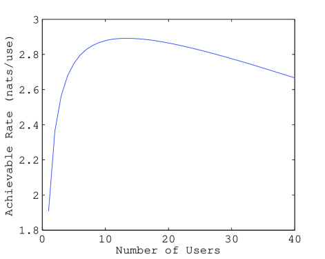
Figure 1: Achievable rate as a function of $K$ with $L=250$

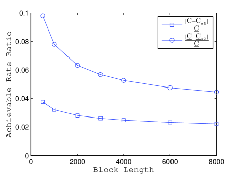
Figure 2: Comparison of $\underline{C}$ to its approximations $\underline{C}_{a1}$ and $\underline{C}_{a2}$

In this section we present numerical results of the system. We use $P=1$, $\sigma_{h}^{2}=1$ and $\sigma_{z}^{2}=0.1$, giving an overall SNR of $S=10$. Figure 1 shows the plot of $\underline{C}$ versus $K$ with the block length fixed at $L=250$. Even with this relatively small block length, only a small proportion of the time is spent training, with the optimal number of users at $K^{*}=14$. In Figure 2 we compare $\underline{C}$ with $\underline{C}_{a1}$ and $\underline{C}_{a2}$ by plotting the corresponding normalized differences (i.e. $\frac{|\underline{C}-\underline{C}_{a1}|}{\underline{C}}$ and $\frac{|\underline{C}-\underline{C}_{a2}|}{\underline{C}}$) for increasing $L$. As expected from Lemma 3, the differences tend to zero in both cases, albeit with slow convergence.

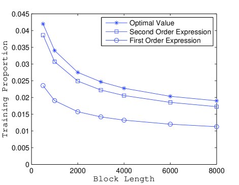
Figure 3: Optimal values and asymptotic expressions for $\alpha$

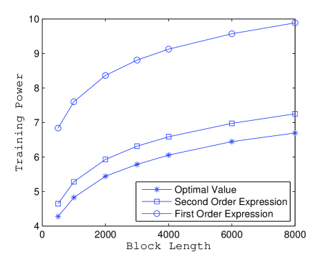
Figure 4: Optimal values and asymptotic expressions for $P_{T}$

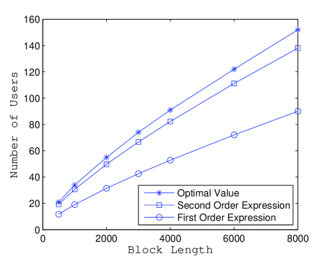
Figure 5: Optimal values and asymptotic expressions for $K$

The scaling of $\alpha^{*}$, $P_{T}^{*}$ and $K^{*}$ are shown in Figures 3, 4 and 5 respectively. The first and second order asymptotic expressions derived in Section IV are shown on the same axes (e.g. the plot of $\alpha$ in Figure 3 uses the expression in (21), giving the first order expression $\frac{S}{S+1}\frac{1}{(\log L)^{2}}$ and second order expression $\frac{S}{S+1}\frac{1}{(\log L)^{2}}+\frac{S(2S+4)}{(S+1)^{2}}\frac{\log\log L}{(\log L)^{3}}$). Although the first order expressions have the same growth rate as the optimal parameters, the gap between the two is reasonable at practical block lengths. On the other hand, the second order parameters approximate the optimal parameters well even at moderate block lengths.

VII Conclusion

We have analyzed a single antenna FDD narrowband MAC with training and user scheduling, using a Rayleigh block fading channel model with independent fading between users. Considering a lower bound on ergodic capacity, a closed form expression has been computed for the optimal proportion of power spent on training, and it has been shown that the optimal training sequence length is $\overline{T}=1$ symbol per user. Second order asymptotic expressions have been obtained for the optimal parameters in terms of $K$ and $L$. Considering the system behavior as $L$ grows large, an approximate expression for the achievable rate has been optimized over $K$, and the resulting second order expressions for the optimized parameters have been obtained.

There are several possible directions for further work. The orthogonal training scheme could be replaced by a more realistic scenario in which the users’ coherence blocks are not aligned. Several different fading models could be considered, including asymmetric statistics and fading distributions other than Rayleigh. With multiple antennas at the base station it would become preferable to allow multiple users to transmit at once [16], adding another level of complexity to the problem. Finally, an interesting problem would be the full analysis of the tradeoff between uplink and downlink rate with training and feedback.

Appendix A Appendix

A-A Proof of Lemma 3

We split this proof into two parts, corresponding to the statements containing $\underline{C}_{a1}$ and $\underline{C}_{a2}$.

A-A1 Expression for $\underline{C}_{a1}$

From (9) and (14) we have $\bar{\epsilon}_{T}^{*}=\Theta(\sqrt{\frac{K}{L}})=o(1)$ and $\alpha^{*}=\frac{K}{L}=o(\bar{\epsilon}_{T}^{*})$, which we substitute into (10) to obtain $x\sim\frac{1}{S}$, or more simply $x=O(1)$. We also note that the values of $K$ which maximize $\underline{C}$ and $\underline{C}_{a1}$ both grow unbounded for large $L$, i.e. $K\rightarrow\infty$. Using these observations, we derive upper and lower bounds such that $\underline{C}\leq\underline{C}_{a1}+o(1)$ and $\underline{C}\geq\underline{C}_{a1}+o(1)$, using the techniques of [9, Proposition 1]. Starting with the upper bound, we apply Jensen’s inequality to (7) to obtain

$$\underline{C}\leq(1-\alpha)\log\left(1+\frac{1}{x}\mathbb{E}\left[|h_{1}^{*}|^{2}\right]\right).$$ (26)

From [17], $\mathbb{E}[|h_{1}^{*}|^{2}]=\sum_{k=1}^{K}\frac{1}{k}$, which is upper bounded by $1+\log(K+1)$. Hence

$$\underline{C}\leq(1-\alpha)\log\left(1+\frac{1}{x}\big{(}\log(K)+O(1)\big{)}\right)$$

$$=\underline{C}_{a1}+(1-\alpha)\log\left(1+O\big{(}\frac{1}{x+\log K}\big{)}\right).$$ (27)

Using $x=O(1)$ and $K\rightarrow\infty$, it is clear that the second term of (27) is $o(1)$.

To obtain a lower bound on $\underline{C}$, we use Markov’s inequality, which states that $\mathbb{E}[X]\geq\Pr(X\geq\beta)\beta$ for any non-negative random variable $X$ and $\beta>0$. Choosing $X=(1-\alpha)\log(1+\frac{1}{x}|h_{1}^{*}|^{2})$ and $\beta=(1-\alpha)\log(1+\frac{1}{x}t)$ where $t$ satisfies $\Pr(|h_{1}^{*}|^{2}\geq t)=1-\frac{1}{\log K}$, the corresponding value of $t$ is the unique solution to

$$1-(1-e^{-t})^{K}=1-\frac{1}{\log K}.$$

It is easy to show that $t=\log K-\log\log\log K$ satisfies this equation asymptotically, and therefore $t=(\log K-\log\log\log K)(1+o(1))$, or more simply $t=\log K+o(\log K)$. Hence the lower bound is

$$\underline{C}\geq\big{(}1-\frac{1}{\log K}\big{)}\big{(}1-\alpha\big{)}\log\left(1+\frac{1}{x}\big{(}\log K+o(\log K)\big{)}\right)$$ (28)

$$=\underline{C}_{a1}+(1-\alpha)\log\left(1+o\big{(}\frac{\log K}{x+\log K}\big{)}\right)+O\left(\frac{\log(1+\frac{1}{x}\log K)}{\log K}\right).$$ (29)

Again, using $x=O(1)$ and $K\rightarrow\infty$, the second and third terms of (29) are $o(1)$. Combining the upper and lower bounds, it follows that $\lim_{L\rightarrow\infty}|\underline{C}-\underline{C}_{a1}|=0$.

A-A2 Expression for $\underline{C}_{a2}$

Substituting (8) into (17) gives

$$\underline{C}_{a1}=\big{(}1-\frac{K}{L}\big{)}\log\left(1+\frac{\sigma_{h}^{2}-\sigma_{e}^{2}}{\sigma_{e}^{2}+\frac{\sigma_{z}^{2}}{P}\frac{1-\alpha}{1-\bar{\epsilon}_{T}}}\log K\right).$$ (30)

We proceed to show that this can be reduced to (18). We define $c_{1}=\sqrt{\frac{S+1}{S}}$ and $c_{2}=\frac{\sigma_{z}^{2}}{P}\sqrt{\frac{S}{S+1}}$, so that $\bar{\epsilon}_{T}^{*}=c_{1}\sqrt{\frac{K}{L}}+O(\frac{K}{L})$ and $(\sigma_{e}^{*})^{2}=c_{2}\sqrt{\frac{L}{K}}+O(\frac{K}{L})$. Substituting these expressions into (30) and applying a sequence of manipulations gives

$$\underline{C}_{a1}=\big{(}1-\frac{K}{L}\big{)}\log\left(1+\frac{\sigma_{h}^{2}-c_{2}\sqrt{\frac{K}{L}}+O(\frac{K}{L})}{c_{2}\sqrt{\frac{K}{L}}+O(\frac{K}{L})+\frac{\sigma_{z}^{2}}{P}\frac{1-K/L}{1-c_{1}\sqrt{K/L}+O(K/L)}}\log K\right)$$ (31)

$$=\big{(}1-\frac{K}{L}\big{)}\log\left(1+\frac{\sigma_{h}^{2}-c_{2}\sqrt{\frac{K}{L}}+O(\frac{K}{L})}{\frac{\sigma_{z}^{2}}{P}+c_{3}\sqrt{\frac{K}{L}}+O(\frac{K}{L})}\log K\right)$$ (32)

$$=\big{(}1-\frac{K}{L}\big{)}\log\left(1+S\big{(}(1-c_{4}\sqrt{\frac{K}{L}}+O(\frac{K}{L})\big{)}\log K\right)$$ (33)

where $c_{3}=c_{2}+\frac{c_{1}\sigma_{z}^{2}}{P}$, $c_{4}=\frac{c_{2}}{\sigma_{h}^{2}}+\frac{Pc_{3}}{\sigma_{z}^{2}}$, and we have used $\frac{1}{1+a}=1-a+O(a^{2})$ as $a\rightarrow 0$. The value of $c_{4}$ can be simplified to $2\sqrt{\frac{S+1}{S}}$, and the expression for $\underline{C}_{a2}$ follows by removing the $O(\frac{K}{L})$ term. To prove that $\lim_{L\rightarrow\infty}|\underline{C}-\underline{C}_{a2}|=0$ is suffices to show that $\lim_{L\rightarrow\infty}|\underline{C}_{a1}-\underline{C}_{a2}|=0$, but this is a simple consequence of the fact that $\frac{K}{L}=o(1)$ and hence the $O(\frac{K}{L})$ term in (33) only contributes an additive $o(1)$ term to $|\underline{C}_{a1}-\underline{C}_{a2}|$.

A-B Proof of Lemma 4

To show that the $O(\frac{K}{L})$ term in (33) is insignificant, we replace it with $d\frac{K}{L}$ for an arbitrary constant $d$, and show that the second order asymptotic expression for $K_{a}^{*}$ does not depend on $d$. We define the resulting expression as

$$\underline{C}{}_{a3}=\big{(}1-\frac{K}{L}\big{)}\log\left(1+S\big{(}1-c\sqrt{\frac{K}{L}}+d\frac{K}{L}\big{)}\log K\right)$$ (34)

where $c=2\sqrt{\frac{S+1}{S}}$. Setting $\frac{\delta}{\delta K}\underline{C}{}_{a3}=0$ gives the necessary condition for $K$ to maximize $\underline{C}_{a3}$,

$$\frac{S(L-K)\left(2(1-c\sqrt{\frac{K}{L}}+d\frac{K}{L})-\log K(c\sqrt{\frac{K}{L}}-2dK\frac{K}{L})\right)}{2K\left(S(1-c\sqrt{\frac{K}{L}}+d\frac{K}{L})\log K+1\right)}=\log\left(1+S\big{(}1-c\sqrt{\frac{K}{L}}+d\frac{K}{L}\big{)}\log K\right).$$ (35)

Hence,

$$\frac{L\big{(}2-c\sqrt{\frac{K}{L}}\log K\big{)}+o(L)+o\big{(}L\sqrt{\frac{K}{L}}\log K\big{)}}{2K\log K+o(K\log K)}=\log\log K+O(1).$$ (36)

It is not immediately obvious whether the dominant term in the numerator of the left hand side of (36) is $2L$ or $-cL\sqrt{\frac{K}{L}}\log K$. The following lemma shows that they in fact have the same first order asymptotic growth rate.

Lemma 6.

A necessary condition for $K$ to satisfy (36) is $\sqrt{\frac{K}{L}}\log K=\Theta(1)$. Furthermore, for sufficiently large $L$ there exists such a solution.

Proof:

We first note that $K=1$ or $K=L$ gives $\underline{C}{}_{a3}=0$, and for large $L$ there always exist values $1<K<L$ such that $\underline{C}{}_{a3}>0$. Combining this with the fact that $\underline{C}{}_{a3}$ is continuous in $K$, $\underline{C}{}_{a3}$ must have a local maximum and therefore (35) must have a solution for large $L$. If $\sqrt{\frac{K}{L}}\log K$ grows faster than $\Theta(1)$, then the numerator of the left hand side of (36) is negative when $L$ is large, which is not possible. If $\sqrt{\frac{K}{L}}\log K=o(1)$, it is easily verified that $L\sim K(\log K)(\log\log K)$, which contradicts the assumption that $\sqrt{\frac{K}{L}}\log K=o(1)$. Therefore $\sqrt{\frac{K}{L}}\log K=\Theta(1)$ is necessary. ∎

Next we define

$$\rho=\sqrt{\frac{K}{L}}\log K$$ (37)

which can be rearranged to obtain

$$L=\frac{1}{\rho^{2}}K(\log K)^{2}.$$ (38)

Substituting (37) and (38) into (36) gives $\frac{1}{\rho^{2}}(1-\frac{\rho c}{2})\log K\sim\log\log K$, which is only possible if $\rho\sim\frac{2}{c}$. Therefore, $L\sim\frac{c^{2}}{4}K(\log K)^{2}$, giving a first order expression for $L$ in terms of $K$. To obtain a second order expression, we set $\rho=\frac{2}{c}+\delta$ and proceed to find a first order expression for $\delta$. From (37) and (38), we obtain

$$1-\frac{c}{2}\sqrt{\frac{K}{L}}\log K=\frac{-c\delta}{2}.$$ (39)

$$L=\frac{c^{2}}{4}\big{(}1-c\delta+O(\delta^{2})\big{)}K(\log K)^{2}$$ (40)

Writing (35) as

$$\frac{L\big{(}1-\frac{c}{2}\sqrt{\frac{K}{L}}\log K\big{)}+O(K\log K)}{K\log K\big{(}1+O(\frac{1}{\log K})\big{)}}=\log\log K+O(1)$$ (41)

and substituting (39) and (40), we obtain

$$\frac{-c^{3}\delta}{8}\log K=\log\log K+O(1).$$ (42)

This implies that $\delta\sim-\frac{8}{c^{3}}\frac{\log\log K}{\log K}$ and hence, from (40),

$$L=\frac{c^{2}}{4}K(\log K)^{2}+2K(\log K)(\log\log K)+O\big{(}K(\log\log K)^{2}\big{)}.$$

Substituting $c=2\sqrt{\frac{S+1}{S}}$ concludes the proof. As previously mentioned, there is no dependence on $d$ in the final expression.

A-C Proof of Theorem 5

For brevity, we write $K$ instead of $K_{a}^{*}$ throughout this section. Several steps will make use of $\frac{1}{1+a}=1-a+O(a^{2})$ and $\log(1+a)=O(a)$ as $a\rightarrow 0$. From (19) we obtain

$$L=\frac{S+1}{S}K(\log K)^{2}\left(1+\frac{2S}{S+1}\frac{\log\log K}{\log K}+O\big{(}(\frac{\log\log K}{\log K})^{2}\big{)}\right)$$ (43)

and consequently

$$\log L=\log K\left(1+\frac{2\log\log K}{\log K}+O\big{(}\frac{1}{\log K}\big{)}\right)$$ (44)

$$\log\log L=\log\log K+O\left(\frac{\log\log K}{\log K}\right).$$ (45)

From (44) and (45) we obtain

$$(\log L)^{2}=(\log K)^{2}+4\log K\log\log K+O(\log K)$$ (46)

$$\frac{\log\log L}{\log L}=\frac{\log\log K}{\log K}+O\left((\frac{\log\log K}{\log K})^{2}\right).$$ (47)

Combining (43) and (46) gives

$$\frac{L}{(\log L)^{2}}=K\frac{S+1}{S}\left(1-\frac{2S+4}{S+1}\frac{\log\log K}{\log K}+O\big{(}\frac{1}{\log K}\big{)}\right)$$

which, when combined with (47), gives the expression for $K_{a}^{*}$ in (20) after solving for $K$ and substituting $O(\frac{1}{\log K})=O(\frac{1}{\log L})$.

We now derive asymptotic expressions for each variable in terms of $L$ after substituting $K$ from (20). The optimal value of $\alpha^{*}$ given by (21) follows immediately from (20) and $\alpha^{*}=\frac{K}{L}$. An alternate expression for $\frac{K}{L}$ is then given by

$$\frac{K}{L}=\frac{S}{S+1}\frac{1}{(\log L)^{2}}\left(1+\frac{2S+4}{S+1}\frac{\log\log L}{\log L}+O\big{(}(\frac{\log\log L}{\log L})^{2}\big{)}\right).$$ (48)

Taking the square root and using $\sqrt{1+a}=1+\frac{a}{2}+O(a^{2})$ as $a\rightarrow 0$,

$$\sqrt{\frac{K}{L}}=\sqrt{\frac{S}{S+1}}\frac{1}{\log L}\left(1+\frac{S+2}{S+1}\frac{\log\log L}{\log L}+O\big{(}(\frac{\log\log L}{\log L})^{2}\big{)}\right).$$ (49)

The final expression for $\bar{\epsilon}_{T}^{*}$ follows from substituting (48) and (49) into (14), and similarly for $(\sigma_{e}^{*})^{2}$ and (24). The expression for $P_{T}^{*}$ follows from substituting the expressions for $\alpha^{*}$ and $\bar{\epsilon}_{T}^{*}$ into $P_{T}^{*}=\frac{\bar{\epsilon}_{T}^{*}P}{\alpha^{*}}$. The expression for $\underline{C}^{*}$ follows from substituting the optimal parameters into (18) and using the result that $|\underline{C}-\underline{C}_{a2}|=o(1)$ from Lemma 3.

References

- [1] R. Knopp and P. A. Humblet, “Information capacity and power control in single-cell multiuser communications,” in IEEE International Conference on Communications, Seattle, WA, June 1995.
- [2] X. Qin and R. A. Berry, “Exploiting multiuser diversity for medium access control in wireless networks,” in IEEE INFOCOM, San Francisco, CA, March 2003.
- [3] S. Sanayei and A. Nosratinia, “Exploiting multiuser diversity with only 1-bit feedback,” in IEEE Wireless Communications and Networking Conference, New Orleans, LA, March 2005.
- [4] M. Sharif and B. Hassibi, “On the capacity of MIMO broadcast channels with partial side information,” IEEE Transactions on Information Theory, vol. 51, no. 2, pp. 506–522, February 2005.
- [5] S. R. Bhaskaran, L. Davis, A. Grant, S. Hanly, and P. Tune, “Downlink scheduling using compressed sensing,” in IEEE Information Theory Workshop on Networking and Information Theory, Voros, Greece, June 2009.
- [6] X. Qin and R. A. Berry, “Distributed approaches for exploiting multiuser diversity in wireless networks,” IEEE Transactions on Information Theory, vol. 52, no. 2, pp. 392–413, February 2006.
- [7] M. Agarwal and M. L. Honig, “Wideband fading channel capacity with training and partial feedback,” IEEE Transactions on Information Theory, vol. 56, no. 10, pp. 4865–4873, October 2010.
- [8] ——, “Spectrum sharing on a wideband fading channel with limited feedback,” in CrownCom International Conference on Cognitive Radio Oriented Wireless Networks and Communications, Orlando, FL, August 2007.
- [9] A. Rajanna and N. Jindal, “Multiuser diversity in downlink channels: When does the feedback cost outweigh the spectral efficiency gain?” http://arxiv.org/abs/1102.1552.
- [10] B. Hassibi and B. M. Hochwald, “How much training is needed in multiple-antenna wireless links?” IEEE Transactions on Information Theory, vol. 49, no. 4, pp. 951–963, April 2003.
- [11] W. Santipach and M. Honig, “Optimization of training and feedback overhead for beamforming over block fading channels,” IEEE Transactions on Information Theory, vol. 56, no. 12, pp. 6103–6115, December 2010.
- [12] M. Kobayashi, N. Jindal, and G. Caire, “How much training and feedback are needed in MIMO broadcast channels?” in IEEE International Symposium on Information Theory, Toronto, Canada, July 2008.
- [13] G. Caire, N. Jindal, M. Kobayashi, and N. Ravindran, “Multiuser MIMO achievable rates with downlink training and channel state feedback,” IEEE Transactions on Information Theory, vol. 56, no. 6, pp. 2845–2866, June 2010.
- [14] M. Medard, “The effect upon channel capacity in wireless communications of perfect and imperfect knowledge of the channel,” IEEE Transactions on Information Theory, vol. 46, no. 3, pp. 933–946, May 2000.
- [15] M. Mecking, “Resource allocation for fading multiple-access channels with partial channel state information,” in IEEE International Conference on Communications, New York, NY, April 2002.
- [16] D. N. C. Tse, P. Viswanath, and L. Zheng, “Diversity-multiplexing tradeoff in multiple-access channels,” IEEE Transactions on Information Theory, vol. 50, no. 9, pp. 1859–1874, September 2004.
- [17] H. A. David and H. N. Nagaraja, Order Statistics, 3rd Edition. New York: John Wiley and Sons, 2003.