Hidden Order and Dynamics in Supersymmetric Valence Bond Solid States
– Super-Matrix Product State Formalism –

Abstract

Supersymmetric valence bond solid models are extensions of the VBS model, a paradigmatic model of ‘solvable’ gapped quantum antiferromagnets, to the case with doped fermionic holes. In this paper, we present a detailed analysis of physical properties of the models. For systematic studies, a supersymmetric version of the matrix product formalism is developed. On 1D chains, we exactly evaluate the hole-doping behavior of various physical quantities, such as the spin/charge excitation spectrum, superconducting order parameter. A generalized hidden order is proposed, and the corresponding string non-local order parameter is also calculated. The behavior of the string order parameter is discussed in the light of the entanglement spectrum.

I Introduction

Valence bond solid (VBS) models introduced by Affleck, Kennedy, Lieb and Tasaki affleck1987rrv; affleck1988vbg are exactly solvable models that exemplify the gapped ground states in integer-$S$ spin chains conjectured by HaldaneHaldane-83a; Haldane-83b. Though the VBS states, which are the exact ground states of the VBS models, are disordered spin liquids in the sense that their spin-spin correlations are exponentially dumped with a very short correlation length, there still exists a certain kind of “hidden order” captured by the non-local string parameterKennedy-T-92a; Kennedy-T-92b. The existence of the hidden order highlights the exotic features of the Haldane-gapped antiferromagnets which are considered as manifestation of the topological order of quantum spin chainArovas-A-H-88; Girvin-A-89; hatsugaiJPSJ1992; Oshikawa-92; Totsuka-S-94; Totsuka-S-mpg-95. With recent increasing interests in the topological states of matter spurred by the discovery of topological insulators [See Ref.qi-2010-63 for instance as a review], the VBS model and its variants are attracting renewed attention. Since the VBS states enable us to calculate many interesting quantities exactly, they offer a rare theoretical playground for the study of topological states of matter. Due to their peculiar features, the VBS-type states have been investigated in a wide variety of contexts like quantum informationwolf-2006-97; perezgarcia-2007-7, topological orderpollmann-2009; Pollmann-T-B-O-10, entanglement entropykatsura-2007-76; katsura-2008-41; xu-2008-133, higher symmetric generalizationsaffleck1991qae; arovas2008sss; greiter2007ers; greiter2007vbs; schuricht2008vbs; Tu08041685; Tu08061839; rachel-2009-86, and topological phase transitions zang-2010-81; zheng-2010.

In this paper, we present a detailed analysis of the recently proposedArovas-H-Q-Z-09 supersymmetric generalization of valence bond solid (sVBS) states. The sVBS states are a precise mathematical realization of Anderson’s scenario of high-$T_{\text{c}}$ conductivityanderson1987rvb and the idea of symmetry unification of superconductivity and antiferromagnetismZhang1997Science. The sVBS states are hole-pair doped VBS states containing both the charge sector and the spin sector; depending on the magnitude of the hole-doping parameter, they exhibit both insulating and superconducting behaviors in the charge sector, while in the spin sector it always displays short-range spin correlationsArovas-H-Q-Z-09.

The effects of mobile holes in the spin-gapped background are interesting in their own right not only in purely theoretical contextZhang-A-89 but also in the experimental point of viewPenc-S-95; xu2000hqs. However, the impact of mobile holes on the (hidden) topological properties has been little studied. In what follows, we will show that the sVBS states possess a kind of non-local topological order in the spin sector as well as local superconducting order in the charge sector, the latter of which is already known. While various (ordinary) correlation functions have been investigated already in Ref.Arovas-H-Q-Z-09, dynamical properties, as exemplified by magnetic- (triplon) and charge (spinon-hole pair, specifically) excitations, are yet to be understood and will also be addressed in this work.

In the sVBS models, supersymmetry (SUSY), i.e. rotational symmetry of boson and fermion, is realized as the symmetry of bosonic spins and fermionic holes. Such SUSY of the sVBS states is exact $\it{regardless}$ $\it{of}$ the magnitude of hole-doping parameter, and their parent Hamiltonians can be readily constructed based on such (super)symmetry. Thus, the sVBS models enable us to systematically study hole-doped antiferromagnets on such a firm mathematical background. To this end, we develop a supersymmetric version of the matrix product state (MPS) representation of the VBS-type statesTotsuka-S-mpg-95. Since the sVBS states generally contain fermionic degrees of freedom, we generalize the MPS formalism to include both fermionic and bosonic operators. This supersymmetric MPS (sMPS) representation is useful not only in the sense of computational efficiency, but also from the topological-order point of view as the emergent edge degrees of freedom, which characterize the topological features, are automatically incorporated in the MPS formalismFannes-N-W-92; Klumper-S-Z-92; Totsuka-S-mpg-95. It should also be mentioned that the MPS formalism, which has been introducedFannes-N-W-92 originally as a special class of quantum ground states with short-range correlations, is now believed to be a natural framework to represent entangled quantum many-body states in 1DVerstraete-C-06; Hastings-area-law-07. In a similar sense, the sMPS formalism would be applicable not only to the sVBS states to be investigated in this paper but to a wider class of entangled many-body states that contain fermionic degrees of freedom.

This paper is structured as follows. In section II, we introduce type I and type II sVBS states and summarize some basic features. In section III, by including fermionic degrees of freedom, we develop the sMPS formalism, and apply it to the calculations of physical quantities of the type I sVBS states. The generalized hidden order is proposed and the string order parameter is evaluated in section IV. In section V, we calculate the gapped excitation spectra of the magnetic- and the charge (i.e. hole-pair) excitations on sVBS chains within the single-mode approximation. In section VI, we proceed to the analysis of type II sVBS states and derive the hole-doping behavior of various physical quantities (e.g. superconducting order parameter and string correlation). The stability of the hidden ‘topological’ order found in these states is discussed from the point of view of the entanglement structure in section VII. Section VIII is devoted to summary and discussions.

II Basic properties

Before proceeding to the detail analysis, we quickly review the basic features of the sVBS states in this section.

II.1 Type I SUSY VBS states

In what follows, we analyze two types of sVBS states. The first is the sVBS states with UOSp(1$|$2) supersymmetry proposed recently in Ref.Arovas-H-Q-Z-09 (see Appendix A, for a very brief summary of supersymmetry), which we shall call type I:

$$|\text{sVBS-I}\rangle=\prod_{\langle ij\rangle}(a_{i}^{\dagger}b_{j}^{\dagger}-b_{i}^{\dagger}a_{j}^{\dagger}-rf_{i}^{\dagger}f_{j}^{\dagger})^{M}|\text{vac}\rangle,$$ (1)

where $\langle ij\rangle$ signifies a pair of adjacent sites $(i,j)$ and $r$ stands for the hole doping parameter. The operators $a_{i}$, $b_{i}$ and $f_{i}$ respectively are a pair of the standard Schwinger bosons satisfying $[a_{i},a^{\dagger}_{j}]=[b_{i},b^{\dagger}_{j}]=\delta_{ij}$ and a (spinless) fermion satisfying $\{f_{i},f^{\dagger}_{j}\}=\delta_{ij}$. The vacuum $|\text{vac}\rangle$ is annihilated by both the boson and the fermion: $a|\text{vac}\rangle=b|\text{vac}\rangle=f|\text{vac}\rangle=0$. Since the fermions always appear in pairs of the form $f_{i}^{\dagger}f_{j}^{\dagger}$ ($i$, $j$ are adjacent), the sVBS states can be regarded as the hole-pair doped VBS states. One can easily see that the state $|\text{sVBS-I}\rangle$ is UOSp(1$|$2)-invariant from the invariance of the matrix

$$\mathcal{R}_{\text{I}}=\begin{pmatrix}0&1&0\\ -1&0&0\\ 0&0&-1\end{pmatrix}$$ (2)

used to construct $|\text{sVBS-I}\rangle$ (The parameter $r$ is absorbed in the renormalization of $f$. To see how the matrix $\mathcal{R}_{\text{I}}$ is related to $|\text{sVBS-I}\rangle$, see section  III.1), and hence $|\text{sVBS-I}\rangle$ has the UOSp(1$|$2) symmetry [See Appendix A.1 for more details].

The type-I sVBS statesArovas-H-Q-Z-09 (1), that contain (fermionic) hole degrees of freedom as well as the (bosonic) spin ones, are a generalization of the standard spin-$S$ VBS statesaffleck1987rrv; affleck1988vbg; Arovas-A-H-88 . In the type-I SVB states (1), the total particle number at each site is conserved:

$$zM=a^{\dagger}_{i}a_{i}+b^{\dagger}_{i}b_{i}+f^{\dagger}_{i}f_{i}\;,$$ (3)

where the lattice coordination number $z$ is $2d$ for the $d$-dimensional hypercubic lattice (in what follows, $z=2$ unless otherwise stated). The integer $zM$ plays a role of the spin quantum number $2S$ in the usual VBS states. Since $f^{\dagger}f$ takes either 0 or 1, the following two eigenvalues are possible for the local spin quantum number $S_{i}=\frac{1}{2}(a^{\dagger}_{i}a_{i}+b^{\dagger}_{i}b_{i})$:

$$S_{i}=M,~{}M-\frac{1}{2}.$$ (4)

In particular, for $M=1$, each site can take two spin values

$$S_{i}=1,~{}\frac{1}{2},$$ (5)

and the local Hilbert space is spanned by the five ($4M{+}1$, in general) basis states

$$\begin{split}&|1\rangle=\frac{1}{\sqrt{2}}{a_{i}^{\dagger}}^{2}|\text{vac}\rangle,\;\;|0\rangle={a_{i}^{\dagger}b_{i}^{\dagger}}|\text{vac}\rangle,\;\;|{-}1\rangle=\frac{1}{\sqrt{2}}{b_{i}^{\dagger}}^{2}|\text{vac}\rangle,\\ &\quad\quad\quad|\!\uparrow\rangle=a_{i}^{\dagger}f_{i}^{\dagger}|\text{vac}\rangle,\;\;|\!\downarrow\rangle=b_{i}^{\dagger}f_{i}^{\dagger}|\text{vac}\rangle\;.\end{split}$$ (6)

Mathematically, these constitute an $\mathcal{N}{=}1$ SUSY multiplet, and hence we use the name ‘Type I’. In addition to the local physical degrees of freedom on each site, the following emergent degrees of freedom localized around the edges (edge states) will play an important role:

$$|\!\uparrow\rangle\!\rangle=a^{\dagger}|\text{vac}\rangle,\;\;|\!\downarrow\rangle\!\rangle=b^{\dagger}|\text{vac}\rangle,\;\;|0\rangle\!\rangle=f^{\dagger}|\text{vac}\rangle.$$ (7)

As we will see in section III.1, the ground state of a finite open chain is 9-fold degenerate (corresponding to the $3\times 3$ matrix for the $M=1$ type-I sVBS states).

The $M=1$ type-I sVBS chain interpolates between the two VBS states in the two extremal limits of the hole doping: at $r\rightarrow 0$, $|\text{sVBS-I}\rangle$ reproduces the original spin-1 VBS state $|\text{VBS}\rangle$affleck1987rrv; affleck1988vbg

$$|\text{sVBS-I}\rangle\rightarrow|\text{VBS}\rangle=\prod_{i}(a^{\dagger}_{i}b_{i+1}^{\dagger}-b_{i}^{\dagger}a_{i+1})|\text{vac}\rangle,$$ (8)

while, in the limit $r\rightarrow\infty$, $|\text{sVBS-I}\rangle$ reduces to the Majumdar-Ghosh (MG) dimer stateMajumdar-G-69; Majumdar-70 $|\text{MG}\rangle$

$$|\text{sVBS-I}\rangle\rightarrow\left\{\prod_{i}f^{\dagger}_{i}\right\}|\text{MG}\rangle,$$ (9)

where $|\text{MG}\rangle$ is either of the two dimerized states of the MG model:

$$|\text{MG}\rangle=\begin{cases}\prod_{i:\text{even}}(a^{\dagger}_{i}b^{\dagger}_{i+1}-b^{\dagger}_{i}a^{\dagger}_{i+1})|\text{vac}\rangle\\ \prod_{i:\text{odd}}(a^{\dagger}_{i}b^{\dagger}_{i+1}-b^{\dagger}_{i}a^{\dagger}_{i+1})|\text{vac}\rangle\;.\end{cases}$$ (10)

For larger $M$, $|\text{MG}\rangle$ should be replaced with the inhomogeneous VBS statesArovas-A-H-88 where the number of valence bonds alternates from bond to bond.

According to the spin-hole coherent state formalism auerbach1994iea, the sVBS state is expressed as

$$\Psi_{\text{sVBS-I}}=\prod_{\langle ij\rangle}(u_{i}v_{j}-v_{i}u_{j}-r\theta_{i}\theta_{j})^{M},$$ (11)

which is simply obtained by replacing the operators $a,b,f$ with their corresponding classical counterparts $u,v,\theta$. ($u,v$ are Grassmann even quantities, while $\theta$ is Grassmann odd.) From the Grassmann odd properties of $\theta$, $\Psi_{\text{sVBS-I}}$ can be rewritten as

$$\Psi_{\text{sVBS-I}}=\exp\biggl{(}-{Mr\sum_{\langle ij\rangle}\frac{\theta_{i}\theta_{j}}{u_{i}v_{j}-v_{i}u_{j}}}\biggr{)}\cdot\Phi_{\text{VBS}}$$ (12)

where $\Phi_{\text{VBS}}=\prod_{\langle ij\rangle}(u_{i}v_{j}-v_{i}u_{j})^{M}$ is the spin coherent state representation of the original VBS state. This expression reminds the BCS wavefunction of the superconductivity; $|\text{BCS}\rangle=\prod_{k}(1+g_{k}c_{k}^{\dagger}c_{-k}^{\dagger})|0\rangle=\exp(\sum_{k}g_{k}c_{k}^{\dagger}c_{-k}^{\dagger})|0\rangle$ with electron operator $c_{k}$ and coherence factor $g_{k}$ (See chapter 2-4 in Ref. SchriefferBook). In both $\Psi_{\text{sVBS-I}}$ and $|\text{BCS}\rangle$, the fermions alway appear in pairs and the wavefunctions can be expressed by a superposition of such fermion pairs, as demonstrated by expanding the exponential (See Fig.1).

Figure 1: The type I sVBS is a superposed state of hole-pair doped VBS states. With finite hole-doping parameter $r$, all of the hole-pair doped VBS states are superposed to form the sVBS state, and the sVBS state exhibits the superconducting property. At $r=0$, the sVBS state is reduced to the original VBS state (depicted as the first chain), while $r\rightarrow\infty$, the sVBS state is reduced to the MG dimer state (depicted as the last two chains).

II.2 Type II sVBS states

The type II sVBS state is an extension of the previous series of VBS states (type I) and now contains doped (antisymmetric) bound pairs of two species of holes. The inclusion of two species of holes $f$ and $g$ allows us to write down a wavefunction more symmetric with respect to the bosonic- and the fermionic degrees of freedom. Now, we introduce the type II sVBS states of the form:

$$|\text{sVBS-II}\rangle=\prod_{\langle ij\rangle}(a_{i}^{\dagger}b_{j}^{\dagger}-b_{i}^{\dagger}a_{j}^{\dagger}-rf_{i}^{\dagger}g_{j}^{\dagger}-rg_{i}^{\dagger}f_{j}^{\dagger})^{M}|\text{vac}\rangle,$$ (13)

which is associated with another matrix:

$${\cal R}_{\text{II}}=\begin{pmatrix}0&1&0&0\\ -1&0&0&0\\ 0&0&0&-1\\ 0&0&-1&0\end{pmatrix}\;.$$ (14)

The new fermion $g_{i}$ satisfies the standard anti-commutation relations $\{g_{i},g^{\dagger}_{j}\}=\delta_{ij}$, $\{f_{i},g_{j}\}=0$, etc. Apparently, the type II sVBS state reduces to the type I after $g_{i}\rightarrow f_{i}$ (and the due rescaling $r\rightarrow\frac{1}{2}r$). With inclusion of another species of the (spinless) hole, in the type II VBS states, there appear the local sites $f^{\dagger}_{i}g_{i}^{\dagger}|0\rangle$ with spin-0, which are not realized in the type I sVBS states. As we will show in the end of this section, the type II sVBS states have the UOSp(2$|$2) symmetry larger than UOSp(1$|$2) symmetry of the type I sVBS states.

We have two species of fermions, and the total particle number at each site $i$ is constrained by

$$zM=a^{\dagger}_{i}a_{i}+b^{\dagger}_{i}b_{i}+f^{\dagger}_{i}f_{i}+g^{\dagger}_{i}g_{i},$$ (15)

where $z$ is the lattice coordination number. Since the eigenvalues of $n_{f}(i){=}f^{\dagger}_{i}f_{i}$ and $n_{g}(i){=}g^{\dagger}_{i}g_{i}$ can take either 0 or 1, in the type II sVBS chain $(z=2)$, the following four eigenvalues are allowed for the local spin quantum number $S_{i}=\frac{1}{2}(a^{\dagger}_{i}a_{i}+b^{\dagger}_{i}b_{i})$:

$$S_{i}={M},~{}M-\frac{1}{2},~{}M-\frac{1}{2},~{}M-1,$$ (16)

which respectively correspond to the possible combinations of the fermion numbers:

$$(n_{f}(i),n_{g}(i))=(0,0),~{}(1,0),~{}(0,1),~{}(1,1)\;.$$ (17)

In particular, for the $M=1$ sVBS chain (i.e. $z=2$), the possible values read

$$S_{i}=1,~{}\frac{1}{2},~{}\frac{1}{2},~{}0\;.$$ (18)

Therefore, the local Hilbert space is spanned by the following nine basis states

$$|1\rangle=\frac{1}{\sqrt{2}}{a_{i}^{\dagger}}^{2}|\text{vac}\rangle,\quad|0\rangle={a_{i}^{\dagger}}b_{i}^{\dagger}|\text{vac}\rangle,\quad|{-1}\rangle=\frac{1}{\sqrt{2}}{b_{i}^{\dagger}}^{2}|\text{vac}\rangle,$$

$$~{}~{}~{}~{}~{}~{}~{}~{}~{}|\!\uparrow\rangle=a_{i}^{\dagger}f_{i}^{\dagger}|\text{vac}\rangle,\quad|\!\downarrow\rangle=b_{i}^{\dagger}f_{i}^{\dagger}|\text{vac}\rangle,$$

$$~{}~{}~{}~{}~{}~{}~{}~{}~{}|\!\uparrow^{\prime}\rangle=a_{i}^{\dagger}g_{i}^{\dagger}|\text{vac}\rangle,\quad|\!\downarrow^{\prime}\rangle=b_{i}^{\dagger}g_{i}^{\dagger}|\text{vac}\rangle,\quad$$

$$~{}~{}~{}~{}~{}~{}~{}~{}~{}~{}~{}~{}~{}~{}~{}~{}~{}~{}|0^{\prime}\rangle=g_{i}^{\dagger}f_{i}^{\dagger}|\text{vac}\rangle.$$ (19)

The name ‘type II’ is indicative of an $\mathcal{N}{=}2$ SUSY multiplet formed by these states. Again, $|\text{vac}\rangle$ denotes the vacuum with respect to $(a,b,f,g)$. The edge states are now given by

$$\begin{split}&|\!\uparrow\rangle\!\rangle=a^{\dagger}|\text{vac}\rangle,\;\;|\!\downarrow\rangle\!\rangle=b^{\dagger}|\text{vac}\rangle,\\ &|0\rangle\!\rangle=f^{\dagger}|\text{vac}\rangle,\;\;|0^{\prime}\rangle\!\rangle=g^{\dagger}|\text{vac}\rangle,\end{split}$$ (20)

and, correspondingly, there appear $4\times 4=16$ degenerate ground states for the $M=1$ type-II sVBS chain (see section  VI for the detail).

The $M=1$ sVBS chain has the following properties. As in the type I sVBS, it reproduces the pure spin VBS state for $r\rightarrow 0$:

$$|\text{sVBS-II}\rangle\rightarrow|\text{VBS}\rangle=\prod_{i}(a^{\dagger}_{i}b_{i+1}^{\dagger}-b_{i}^{\dagger}a^{\dagger}_{i+1})|\text{vac}\rangle\;.$$ (21)

On the other hand, when $r\rightarrow\infty$, it reduces to the totally uncorrelated fermionic (F) state filled with holes:

$$\begin{split}|\text{sVBS-II}\rangle\rightarrow|\text{F-VBS}\rangle&\equiv\prod_{i}(f^{\dagger}_{i}g^{\dagger}_{i+1}+g^{\dagger}_{i}f^{\dagger}_{i+1})|\text{vac}\rangle\\ &=\pm\prod_{i}f^{\dagger}_{i}g^{\dagger}_{i}|\text{vac}\rangle\end{split}$$ (22)

(the sign factor depends on both the parity of the system size and the edge states). Here we have assumed the open boundary condition and the normalization of the edge states given in section  VI.1.

This properties are quite similar to those of the BCS state; at $g_{k}\rightarrow 0$, the BCS state reduces to the electron vacuum (no fermions), while for $g_{k}\rightarrow\infty$, it coincides with the Fermi sphere (filled with electrons). In this sense, the type II sVBS states look more similar to the BCS state than the type I VBS states. As in the previous case, one can pursue the analogy to the BCS wave function by using the spin-hole coherent state representation of $|\text{sVBS-II}\rangle$:

$$\Psi_{\text{sVBS-II}} =\prod_{<ij>}(u_{i}v_{j}-v_{i}u_{j}-r\theta_{i}\eta_{j}-r\eta_{i}\theta_{j})^{M}$$

$$=\exp\biggl{(}-Mr\sum_{<ij>}\frac{\theta_{i}\eta_{j}+\eta_{i}\theta_{j}}{u_{i}v_{j}-v_{i}u_{j}}\biggr{)}$$

$$~{}~{}\cdot\exp\biggl{(}-Mr^{2}\sum_{<ij>}\frac{\theta_{i}\eta_{i}\theta_{j}\eta_{j}}{(u_{i}v_{j}-v_{i}u_{j})^{2}}\biggr{)}{\cdot}\Phi_{\text{VBS}}.$$ (23)

Expanding the exponentials, one can easily see that with finite $r$, the type II sVBS states can be expressed as a superposition of the hole-pair-doped VBS states and that the system exhibits the superconducting property. However, unlike type I, type II sVBS states have no spin degrees of freedom at $r\rightarrow\infty$. The intuitive picture of the $M=1$ type II sVBS chain is depicted in Fig.2.

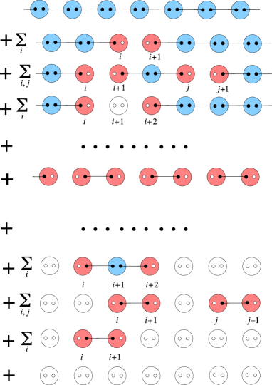
Figure 2: (color online) The type II sVBS states are expressed as superposition of the hole-pair doped VBS states. Unlike the type I sVBS states, the spinless sites, depicted by the large white circles with double holes, appear. The MG states are realized in the “middle” of the sequence. The original VBS state and the hole-VBS state are respectively realized in the first and last lines.

Before concluding this section, we give a remark about the symmetry of the type II sVBS state. In Ref. Arovas-H-Q-Z-09, an apparently different form of the sVBS states

$$|\text{sVBS}^{\prime}\rangle=\prod_{\langle ij\rangle}(a_{i}^{\dagger}b_{j}^{\dagger}-b_{i}^{\dagger}a_{j}^{\dagger}-rf_{i}^{\dagger}f_{j}^{\dagger}-rg_{i}^{\dagger}g_{j}^{\dagger})^{M}|\text{vac}\rangle,$$ (24)

has been introduced. The state $|\text{sVBS}^{\prime}\rangle$ is manifestly invariant under the UOSp(2$|$2) transformation, since it is constructed by using the UOSp(2$|$2)-invariant matrix

$$\mathcal{R}^{\prime}=\begin{pmatrix}0&1&0&0\\ -1&0&0&0\\ 0&0&-1&0\\ 0&0&0&-1\end{pmatrix}\;.$$ (25)

($r$ can be absorbed in the normalization of $f$ and $g$.) In fact, the two sVBS states $|\text{sVBS-II}\rangle$ and $|\text{sVBS'}\rangle$ are physically equivalent. By the unitary transformation

$$\begin{pmatrix}f^{\dagger}\\ g^{\dagger}\end{pmatrix}\rightarrow\frac{1}{\sqrt{2}}\begin{pmatrix}1&-1\\ 1&1\end{pmatrix}\begin{pmatrix}f^{\dagger}\\ g^{\dagger}\end{pmatrix},$$ (26)

the fermion-pair part of $|\text{sVBS-II}\rangle$ is transformed to

$$f_{i}^{\dagger}g_{j}^{\dagger}+g_{i}^{\dagger}f_{j}^{\dagger}\longrightarrow f_{i}^{\dagger}f_{j}^{\dagger}-g_{i}^{\dagger}g_{j}^{\dagger}.$$ (27)

Then, we flip the sign of either $g_{i}^{\dagger}$ or $g_{j}^{\dagger}$ to recover the correct form of the fermion-pair part in $|\text{sVBS}^{\prime}\rangle$:

$$f_{i}^{\dagger}f_{j}^{\dagger}-g_{i}^{\dagger}g_{j}^{\dagger}\longrightarrow f_{i}^{\dagger}f_{j}^{\dagger}+g_{i}^{\dagger}g_{j}^{\dagger}.$$ (28)

As the phase of the operators can be chosen arbitrarily, flipping the sign of them does not affect physics. Therefore, both $|\text{sVBS-II}\rangle$ and $|\text{sVBS}^{\prime}\rangle$ have the same symmetry UOSp(2$|$2) in common and are physically equivalent; all physical quantities take completely identical values for these two statessupp.

III SUSY-VBS state-I

In the following sections, we consider the sVBS states defined on one-dimensional (1D) chain. A simplest SUSY-extension of the 1D spin-1 AKLT (VBS) stateaffleck1987rrv; affleck1988vbg is defined as ($M=1$, $z=2$ in eq.(1)):

$$\begin{split}|\text{sVBS-I}\rangle\equiv&(\cdots)(a^{\dagger}_{j-1}b^{\dagger}_{j}-b^{\dagger}_{j-1}a^{\dagger}_{j}-r\,f^{\dagger}_{j-1}f^{\dagger}_{j})\\ &(a^{\dagger}_{j}b^{\dagger}_{j+1}-b^{\dagger}_{j}a^{\dagger}_{j+1}-r\,f^{\dagger}_{j}f^{\dagger}_{j+1})(\cdots)|\text{vac}\rangle\;.\end{split}$$ (29)

The (non-hermitian) parent Hamiltonian for the SUSY (UOSp($1|2$)) VBS model is given asArovas-H-Q-Z-09:

$$\widetilde{{\cal H}}_{l=1\text{ sVBS}}=\sum_{j}\left\{V_{3/2}P_{3/2}({\cal C}_{j,j+1})+V_{2}P_{2}({\cal C}_{j,j+1})\right\}\;,$$ (30)

where ${\cal C}_{j,j+1}$ and $P_{l}({\cal C}_{j,j+1})$ respectively denote the UOSp($1|2$) Casimir operator on a two-site cluster $(j,j+1)$ (see eqs.(111,115) for the definition of Casimir operators) and the projection operator onto $l_{\text{tot}}=l$ subspace (note that the total superspin $l_{\text{tot}}$ of two $l=1$ superspins can take all integer- and half-integer values between 0 and 2; see eq.(116)). For the positivity of the Hamiltonian, we require $V_{3/2},V_{2}\gneq 0$. Specifically, the local Hamiltonian $h_{j,j+1}$ is given by the following fourth-order polynomial of the Casimir ${\cal C}_{j,j+1}$:

$$h({\cal C})=\left(\frac{V_{3/2}}{6}-\frac{V_{2}}{70}\right){\cal C}+\left(\frac{3V_{2}}{70}-\frac{43V_{3/2}}{90}\right){\cal C}^{2}\\ +\left(\frac{14V_{3/2}}{45}-\frac{2V_{2}}{63}\right){\cal C}^{3}+\left(\frac{2V_{2}}{315}-\frac{2V_{3/2}}{45}\right){\cal C}^{4}\;.$$ (31)

III.1 Matrix-product representation

First let us briefly recapitulate the basic properties of a generic (bosonic) matrix-product state of the following form (see, for instance, Refs. perezgarcia-2007-7; Verstraete-M-C-08 for recent reviews of the matrix-product representations):

$$|\text{MPS}\rangle=\bigotimes_{j=1}^{L}A_{j}\;,$$ (32a)

where the matrix $$A_{j} j |\text{MPS}\rangle |\text{MPS}\rangle |\text{sVBS}\rangle S (S{+}1){\times}(S{+}1)$$ consists of state vectors at the site- and its size is determined solely by the size of the auxiliary Hilbert space and is independent of the number of sites. The state in general is not normalized and we reserve the notation (and ) for the unnormalized states. Ground states which can be expressed in this form may be generically expected to have finite degeneracy. For example, the ground state of the AKLT model, which is expressed by the spin- VBS state, is shownaffleck1987rrv; affleck1988vbg to have -fold degenerate, when the model is defined on a finite open chain. When the system is defined on a periodic chain, we have to take the trace over the matrix indices:

$$|\text{MPS}\rangle_{\text{PBC}}=\text{Tr}\left\{\bigotimes_{j=1}^{L}A_{j}\right\}\;,$$ (32b)

Below, we shall see that the expression eq.(32b) should be modified when $A$ contains both bosonic degrees of freedom and fermionic ones.

Now let us construct the matrix-product representationFannes-N-W-89; Fannes-N-W-92 of the type I (UOSp(1$|$2)) VBS state (29). When the Schwinger-boson/fermion representation of the state is known, the simplest wayTotsuka-S-94 would be to find an operator-valued matrix in such a way that everytime when we multiply a new matrix (say, $g_{j+1}$) from the right the (SUSY) valence-bond operator

$$(a^{\dagger}_{j}b^{\dagger}_{j+1}-b^{\dagger}_{j}a^{\dagger}_{j+1}-r\,f^{\dagger}_{j}f^{\dagger}_{j+1})$$

is inserted between the previous right edge (site-$j$) and the newly added site ($j{+}1$). To this end, let us introduce the ‘spinor’:

$$\psi_{j}=(a^{\dagger}_{j},b^{\dagger}_{j},\sqrt{r}f_{j}^{\dagger})^{\text{t}}\;,$$ (33)

in terms of which the above UOSp(1$|$2) valence bond can be written compactly as:

$$(a^{\dagger}_{j}b^{\dagger}_{j+1}-b^{\dagger}_{j}a^{\dagger}_{j+1}-r\,f^{\dagger}_{j}f^{\dagger}_{j+1})=\psi_{j}^{\text{t}}{\cal R}_{\text{I}}\psi_{j+1}$$ (34)

(‘t’ denotes the transposition). The ‘metric’ ${\cal R}_{\text{I}}$ has been defined as

$${\cal R}_{\text{I}}=\begin{pmatrix}0&1&0\\ -1&0&0\\ 0&0&-1\end{pmatrix}\;.$$ (35)

Then the sVBS state (29) is written as a string of 3$\times$3 matrices $(\alpha,\beta=1,2,3)$:

$$\begin{split}|\text{sVBS}\rangle_{\alpha\beta}&=({\cal R}_{\text{I}}\psi_{1})^{\alpha}\prod_{i=1}^{L-1}(\psi_{i}^{\text{t}}\mathcal{R}_{\text{I}}\psi_{i+1})\psi^{\beta}_{L}|\text{vac}\rangle\\ &\equiv({\cal R}_{\text{I}}\psi_{1})^{\alpha}\psi_{1}^{\text{t}}\cdot\left(\prod_{i=2}^{L-1}\mathcal{R}_{\text{I}}\psi_{i}\psi_{i}^{\text{t}}\right)\cdot({\cal R}_{\text{I}}\psi_{L}\psi_{L}^{\beta})|\text{vac}\rangle\\ &=(A_{1}A_{2}\cdots A_{L})_{\alpha\beta},\end{split}$$ (36)

where

$$\begin{split}A_{j}&=\mathcal{R}_{\text{I}}\psi_{j}\cdot\psi_{j}^{\text{t}}|\text{vac}\rangle_{j}\\ &=\begin{pmatrix}a_{j}^{\dagger}b_{j}^{\dagger}&(b_{j}^{\dagger})^{2}&\sqrt{r}b_{j}^{\dagger}f_{j}^{\dagger}\\ -(a_{j}^{\dagger})^{2}&-a_{j}^{\dagger}b_{j}^{\dagger}&-\sqrt{r}a_{j}^{\dagger}f_{j}^{\dagger}\\ -\sqrt{r}f_{j}^{\dagger}a_{j}^{\dagger}&-\sqrt{r}f_{j}^{\dagger}b_{j}^{\dagger}&0\end{pmatrix}|\text{vac}\rangle_{j}\\ &=\begin{pmatrix}|0\rangle_{j}&\sqrt{2}|{-1}\rangle_{j}&\sqrt{r}|\!\downarrow\rangle_{j}\\ -\sqrt{2}|1\rangle_{j}&-|0\rangle_{j}&-\sqrt{r}|\!\uparrow\rangle_{j}\\ -\sqrt{r}|\!\uparrow\rangle_{j}&-\sqrt{r}|\!\downarrow\rangle_{j}&0\end{pmatrix}\\ &\equiv\sum_{m=-1,0,1}\Gamma^{(\text{B})}(m)|m\rangle+\sum_{\widetilde{m}=\uparrow,\downarrow}\Gamma^{(\text{F})}(\widetilde{m})|\widetilde{m}\rangle\;.\end{split}$$ (37)

The 3$\times$3 matrices $\Gamma^{(\text{B})}$ and $\Gamma^{(\text{F})}$ respectively denote the bosonic- and the fermionic part. The edge operators ${\cal R}_{\text{I}}\psi_{1}=(b_{1}^{\dagger},-a_{1}^{\dagger},-\sqrt{r}f_{1}^{\dagger})^{\text{t}}$ and $\psi_{L}$ appearing respectively on the left- and the right edge represent the three possible edge states (spin-up/down and hole) on each edge.

Following the same steps as the above for

$$\begin{split}\langle\text{sVBS-I}|=&\langle\text{vac}|(\cdots)(a_{j}b_{j+1}-b_{j}a_{j+1}-r\,f_{j+1}f_{j})\\ &(a_{j-1}b_{j}-b_{j-1}a_{j}-r\,f_{j}f_{j-1})(\cdots)\;,\end{split}$$ (38)

we obtain

$${}_{\alpha\beta}\langle\text{sVBS-I}|=\left(A_{L}^{\dagger}A_{L-1}^{\dagger}\cdots A_{2}^{\dagger}A_{1}^{\dagger}\right)_{\beta\alpha}$$ (39)

with

$$\begin{split}A^{\dagger}_{j}&={}_{j}\langle\text{vac}|\psi^{\ast}_{j}\psi^{\dagger}_{j}{\cal R}^{\text{t}}\\ &={}_{j}\langle\text{vac}|\begin{pmatrix}a_{j}b_{j}&-(a_{j})^{2}&-\sqrt{r}a_{j}f_{j}\\ (b_{j})^{2}&-a_{j}b_{j}&-\sqrt{r}b_{j}f_{j}\\ \sqrt{r}f_{j}b_{j}&-\sqrt{r}f_{j}a_{j}&0\end{pmatrix}\;,\end{split}$$ (40)

where $\psi^{\ast}_{j}\equiv(a_{j},b_{j},\sqrt{r}f_{j})^{\text{t}}$.

By construction, it is obvious that all the nine matrix elements of the following string of $A$-matrices:

$$\bigotimes_{j=1}^{L}A_{j}\\ =\begin{pmatrix}b^{\dagger}_{1}\\ -a^{\dagger}_{1}\\ -\sqrt{r}f^{\dagger}_{1}\end{pmatrix}\left\{\prod_{j=1}^{L-1}(a^{\dagger}_{j}b^{\dagger}_{j+1}-b^{\dagger}_{j}a^{\dagger}_{j+1}-r\,f^{\dagger}_{j}f^{\dagger}_{j+1})\right\}\\ \times\begin{pmatrix}a^{\dagger}_{L}&b^{\dagger}_{L}&\sqrt{r}f^{\dagger}_{L}\end{pmatrix}|\text{vac}\rangle$$ (41)

are the (zero-energy) ground states of the parent Hamiltonian $\sum_{j=1}^{L-1}h_{j,j+1}$. That is, the product $\bigotimes_{j=1}^{L}A_{j}$ gives the the ground states of the $M=1$ sVBS model on an open chain with length $L$. Here it is important to note that we are free to choose the polynomials ($\begin{pmatrix}b^{\dagger}_{1}&-a^{\dagger}_{1}&-\sqrt{r}f^{\dagger}_{1}\end{pmatrix}$ from the left edge and $\begin{pmatrix}a^{\dagger}_{L}&b^{\dagger}_{L}&\sqrt{r}f^{\dagger}_{L}\end{pmatrix}$ from the right) appearing at the edges. As will be discussed in section III.2, this leads to a remarkable feature of the VBS-like systems–edge states.

In constructing the sVBS state on a periodic chain, one has to treat the fermion sign carefully and one sees that the trace operation used in the standard MPS representation (32b) should be replaced with the supertrace (see Appendix B):

$$|\text{sVBS}\rangle_{\text{periodic}}=\text{STr}\left\{\bigotimes_{j=1}^{L}A_{j}\right\}\;,$$ (42a)

where the supertrace here is defined as

$$\text{STr}({\cal M})\equiv{\cal M}_{11}+{\cal M}_{22}-{\cal M}_{33}\;.$$ (42b)

From these $A$-matrices, we can calculate the following 9$\times$9 $T$-matrices (transfer matrix):

$$\begin{split}&T(\bar{\alpha},\alpha;\bar{\beta},\beta)\equiv A^{\ast}(\bar{\alpha},\bar{\beta})A(\alpha,\beta)\\ &=\left(\begin{array}[]{lllllllll}1&0&0&0&2&0&0&0&r\\ 0&-1&0&0&0&0&0&0&0\\ 0&0&0&0&0&0&0&-r&0\\ 0&0&0&-1&0&0&0&0&0\\ 2&0&0&0&1&0&0&0&r\\ 0&0&0&0&0&0&r&0&0\\ 0&0&0&0&0&-r&0&0&0\\ 0&0&r&0&0&0&0&0&0\\ r&0&0&0&r&0&0&0&0\end{array}\right)\\ &\quad(\bar{\alpha},\alpha,\bar{\beta},\beta=1,2,3)\;,\end{split}$$ (43)

where $A^{\ast}$ is obtained from $A$ by $|\cdot\rangle\mapsto\langle\cdot|$ and complex conjugation. The eigenvalues of $T$ are

$$\biggl{\{}-1(\times 3),-ir(\times 2),ir(\times 2),\\ \frac{1}{2}\left(3-\sqrt{8r^{2}+9}\right),\frac{1}{2}\left(3+\sqrt{8r^{2}+9}\right)\biggr{\}}\;.$$ (44)

The largest eigenvalue which is relevant in determining the physical quantities in the thermodynamic limit is given, for any finite $r$, by

$$\frac{1}{2}\left(3+\sqrt{8r^{2}+9}\right)\;.$$ (45)

In the limit $r\rightarrow\infty$, another eigenvalue $\left(3-\sqrt{8r^{2}+9}\right)/2$ becomes degenerate with the above.

The use of the supertrace in eq.(42a) modifies the expression (127) of the norm for the periodic system to:

$$\langle\text{MPS}|\text{MPS}\rangle_{\text{PBC}}=\sum_{\alpha,\beta}\text{sgn}(\alpha)\text{sgn}(\beta)\left\{T^{L}\right\}_{(\alpha,\beta;\alpha,\beta)}\;,$$ (46a)

where

$$\text{sgn}(\alpha)=\begin{cases}1&\text{for }\alpha=1,2\\ -1&\text{for }\alpha=3\;.\end{cases}$$ (46b)

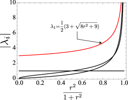
Figure 3: (Color online) Plot of absolute values of the five different eigenvalues of $T$. The largest eigenvalue is always unique and non-degenerate.

III.2 Edge states

Now we would like to mention an important feature of the VBS-like states defined on an open chain. From the expression (41), it is clear that the nine degenerate ground states correspond to different choices of the edge polynomials $(b^{\dagger}_{1},\,-a^{\dagger}_{1},\,-\sqrt{r}f^{\dagger}_{1})$ and $(a^{\dagger}_{L},\,b^{\dagger}_{L},\,\sqrt{r}f^{\dagger}_{L})$. In fact, we can explicitly indicate the edge-dependence of the ground states as follows:

$$\begin{split}&|\text{sVBS}\rangle_{\text{open}}=\bigotimes_{j=1}^{L}A_{j}\\ &=\begin{pmatrix}|s_{\text{L}}{=}\downarrow;s_{\text{R}}{=}\uparrow\rangle&|s_{\text{L}}{=}\downarrow;s_{\text{R}}{=}\downarrow\rangle&|s_{\text{L}}{=}\downarrow;s_{\text{R}}{=}\circ\rangle\\ |s_{\text{L}}{=}\uparrow;s_{\text{R}}{=}\uparrow\rangle&|s_{\text{L}}{=}\uparrow;s_{\text{R}}{=}\downarrow\rangle&|s_{\text{L}}{=}\uparrow;s_{\text{R}}{=}\circ\rangle\\ |s_{\text{L}}{=}\circ;s_{\text{R}}{=}\uparrow\rangle&|s_{\text{L}}{=}\circ;s_{\text{R}}{=}\downarrow\rangle&|s_{\text{L}}{=}\circ;s_{\text{R}}{=}\circ\rangle\\ \end{pmatrix}\;.\end{split}$$ (47)

From this, we can readily see that the matrix indices of the MPS are directly related to the edge states. It is instructive to calculate $\langle S^{z}_{j}\rangle$ for various edge states $|\text{sVBS}\rangle_{\text{open}}^{(s_{\text{L}},s_{\text{R}})}$. In Fig. 4, we plot the local magnetization $\langle S^{z}_{j}\rangle$ for three left edge states $s_{\text{L}}$ (with the right edge state $s_{\text{R}}$ fixed).

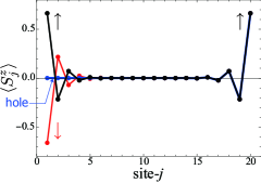
Figure 4: (Color online) Plot of $\langle S^{z}_{j}\rangle$ ($r=0.3$) for various (left) edge states ‘hole’, ‘$\uparrow$’ and ‘$\downarrow$’ (with the right edge state fixed to $s_{\text{R}}=\uparrow$). The system is non-magnetic in the bulk and magnetic moment exists only around the edges of the chain.

A remark is in order here. One may think of the above edge moments ($s=1/2$ moment or a hole) as independent physical objects and conclude that the (SUSY) VBS states are orthogonal with respect to these edge states. However, this is not true; in fact, the above edge moments are emergent objects and sVBS states with different edge states have finite overlaps with each other, which are exponentially decreasing as the system size $L$. That is, two VBS states with different edge states are orthogonal to each other only in the infinite-size limit. In the MPS formulation, this is a direct consequence of the fact

$$[T^{n}]_{(\alpha_{\text{L}},\beta_{\text{L}};\alpha_{\text{R}},\beta_{\text{R}})}\xrightarrow{n\nearrow\infty}\delta_{\alpha_{\text{L}},\beta_{\text{L}}}\delta_{\alpha_{\text{R}},\beta_{\text{R}}}\times{\cal F}_{\alpha_{\text{L}},\alpha_{\text{R}}}(r)\;.$$ (48)

In fact, this property greatly simplifies the calculations below.

III.3 Spin-spin correlation

Now that we have obtained all the necessary matrices, we can follow the steps described in section B.2 to calculate various correlation functions.

The ordinary spin-spin correlation function $\langle S^{a}_{x}S^{a}_{x+n}\rangle$ reads:

$$\frac{2\left(r^{2}+3+\sqrt{8r^{2}+9}\right)}{\sqrt{8r^{2}+9}\left(3+\sqrt{8r^{2}+9}\right)}\quad(\text{for }n=0)$$ (49a)

$$\begin{split}&\frac{13r^{2}+24+\left(r^{2}+8\right)\sqrt{8r^{2}+9}}{2\sqrt{8r^{2}+9}\left(3+\sqrt{8r^{2}+9}\right)}\left(-\frac{2}{3+\sqrt{8r^{2}+9}}\right)^{n}\\ &\qquad(\text{for }n>0)\;.\end{split}$$ (49b)

The exponentially decaying factor defines the correlation lengthArovas-H-Q-Z-09:

$$\xi_{\text{spin}}(r)^{-1}\equiv\log\left\{\frac{3+\sqrt{8r^{2}+9}}{2}\right\}\;,$$ (50)

which is monotonically decreasing in $r$. In the pure AKLT-limit $r\rightarrow 0$, it reduces to the well-known resultsaffleck1987rrv; affleck1988vbg:

$$\langle S^{a}_{x}S^{a}_{x+n}\rangle=\begin{cases}\frac{2}{3}\quad&\text{for }n=0\\ \frac{4}{3}\left(\frac{-1}{3}\right)^{n}\quad&\text{for }n>0\;.\end{cases}$$ (51)

For later convenience, we calculate the static structure factor $S^{\alpha\alpha}(k)$. The result is given as:

$$S^{zz}(k)=\frac{4\left(2r^{4}+17r^{2}+\left(3r^{2}+6\right)\sqrt{8r^{2}+9}+18\right)(1-\cos(k))}{\sqrt{8r^{2}+9}\left(\sqrt{8r^{2}+9}+3\right)\left\{4r^{2}+3\sqrt{8r^{2}+9}+11+2\left(\sqrt{8r^{2}+9}+3\right)\cos(k)\right\}}.$$ (52)

III.4 superconducting correlation

In order to handle the operators containing fermions, we have to generalize the general recipe presented in Appendix B. Take for example the hole-pair creation operatorArovas-H-Q-Z-09:

$$\begin{split}\Delta_{j}&\equiv(a_{j}b_{j+1}-b_{j}a_{j+1})f^{\dagger}_{j}f^{\dagger}_{j+1}\\ &=(a_{j}f^{\dagger}_{j})(b_{j+1}f^{\dagger}_{j+1})-(b_{j}f^{\dagger}_{j})(a_{j+1}f^{\dagger}_{j+1})\;.\end{split}$$ (53)

In order to apply the method presented in sections B.1 and B.2, first a string of $A$-matrices $A_{1}\otimes\cdots\otimes A_{j}$ has to be moved to the left of $f^{\dagger}_{j+1}$ and through this procedure it acquires a Jordan-Wigner-like phase $\prod_{k=1}^{j}(-1)^{F_{k}}$ ($F_{k}$ counts the fermion number 0 or 1 at the site $k$; see Fig.5):

$$(-1)^{F_{1}}A_{1}\otimes\cdots\otimes(-1)^{F_{j}}A_{j}\;.$$ (54)

Next a string $(-1)^{F_{1}}A_{1}\otimes\cdots\otimes(-1)^{F_{j-1}}A_{j-1}$ and $f^{\dagger}_{j}$ are interchanged and this multiplies the matrices $A_{1}$, …, $A_{j-1}$ additional $(-1)^{F_{k}}$-factors to remove the fermion sign except at the site $j$. Therefore, we need four more matrices

$$\begin{split}&T^{\mathcal{O}f^{\dagger}}(\bar{\alpha},\alpha;\bar{\beta},\beta)\equiv A^{\ast}(\bar{\alpha},\bar{\beta})(\mathcal{O}f^{\dagger})A(\alpha,\beta)\;,\\ &\widetilde{T}^{\mathcal{O}f^{\dagger}}(\bar{\alpha},\alpha;\bar{\beta},\beta)\equiv A^{\ast}(\bar{\alpha},\bar{\beta})\left\{\mathcal{O}f^{\dagger}(-1)^{F}\right\}A(\alpha,\beta)\\ &\phantom{\widetilde{T}^{\beta f^{\dagger}}(\bar{m},m;\bar{n},n)\equiv A^{\ast}(\bar{m},\bar{n})g(m,n)}(\mathcal{O}=a,b)\;.\end{split}$$ (55)

By using these, the numerator of $\langle\Delta_{j}\rangle$ is calculated as:

$$T^{j-1}\left\{\widetilde{T}^{af^{\dagger}}T^{bf^{\dagger}}-\widetilde{T}^{bf^{\dagger}}T^{af^{\dagger}}\right\}T^{l-j-1}\;.$$ (56)

Also interesting are the hole density

$$\langle n_{\text{hole}}\rangle=\langle f^{\dagger}_{j}f_{j}\rangle$$ (57)

and the hole-number fluctuation

$$\delta n_{\text{hole}}=\sqrt{\langle f^{\dagger}_{j}f_{j}\rangle-\langle f^{\dagger}_{j}f_{j}\rangle^{2}}\;.$$ (58)

By using the method described above, we can readily calculate these quantities. For instance, the hole density in the bulk system is computed as:

$$\langle n_{\text{hole}}\rangle=\frac{r^{2}(5+\sqrt{8r^{2}+9})}{8r^{2}+9+\left(r^{2}+3\right)\sqrt{8r^{2}+9}}\;.$$ (59)

As is clearly seen in the inset of Fig. 6, near the edges of an open chain, the hole density is different from the bulk value and approaches exponentially with the ‘healing length’ given by

$$\xi_{\text{hole}}(r)^{-1}=\log\left\{\frac{\sqrt{8r^{2}+9}+3}{\sqrt{8r^{2}+9}-3}\right\}\;.$$ (60)

Note that this is different from the spin correlation length $\xi_{\text{spin}}(r)$ in eq.(50) and the superconducting correlation length

$$\xi_{\text{sc}}(r)=1/\log\left\{\frac{\sqrt{8r^{2}+9}+3}{2r}\right\}$$ (61)

defined by the exponential decay of the singlet off-diagonal correlation functionArovas-H-Q-Z-09 $\langle(a_{j}b_{j+n}-b_{j}a_{j+n})f^{\dagger}_{j}f^{\dagger}_{j+n}\rangle$.

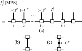
Figure 5: Action of fermion operator on the MPS. (a): Due to the fermionic anticommutation relation, extra factors $(-1)^{F}$ appear in the $A$-matrices on the left of site-$j$. Accordingly, a new transfer matrix (c) is necessary as well as the standard one (b) when we calculate expectation values containing fermionic operators.

In Fig.6, we plot the expectation value of the hole-pair creation operator:

$${\cal O}_{\text{sc}}\equiv\langle\Delta_{j}\rangle$$ (62)

together with the hole density $\langle n_{\text{hole}}\rangle=\langle f^{\dagger}_{j}f_{j}\rangle$ and the hole-number fluctuation $\delta n_{\text{hole}}=\sqrt{\langle f^{\dagger}_{j}f_{j}\rangle-\langle f^{\dagger}_{j}f_{j}\rangle^{2}}$. From $r=0$ ($S=1$ VBS limit) to $r\rightarrow\infty$ ($S=1/2$ Majumdar-Ghosh limit), the hole density is monotonically increasing. When $r=0$ and $r\rightarrow\infty$, the hole number fluctuation is suppressed ($n_{\text{hole}}$ takes definite values 0 and 1, respectively) and consequently the ‘superconducting correlation’ becomes zero. This is consistent with what we expect from the analogy to the BCS wave function pointed out in Ref.Arovas-H-Q-Z-09.

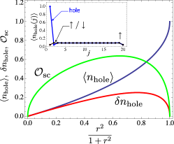
Figure 6: (Color online) Plot of ${\cal O}_{\text{sc}}=\langle\Delta_{j}\rangle$, the hole density $\langle n_{\text{hole}}(j)\rangle=\langle f^{\dagger}_{j}f_{j}\rangle$ and the hole-number fluctuation $\langle f^{\dagger}_{j}f_{j}\rangle-\langle f^{\dagger}_{j}f_{j}\rangle^{2}$ as a function of $r$. Here the bulk values are plotted. Inset: Profile of the hole density ($r=0.5$) for a finite system ($L=20$) with different left edge states ($\uparrow$, $\downarrow$, and ‘hole’). Only the left edge state is changed with the right one fixed to $s_{\text{R}}=\uparrow$. The hole density approaches exponentially to the bulk value as we move away from the edge.

IV Hidden order

IV.1 Generalized Hidden Order in sVBS states

The hidden order is a generalized concept of the Néel order. For $S=1$ antiferromagnetic spin chain, the Néel order is depicted as

$$\cdots~{}+~{}-~{}+~{}-~{}+~{}-~{}+~{}-~{}+~{}\cdots$$ (63)

Here, $+$ stands for $S_{z}=+1$, and $-$ for $S_{z}=-1$. In the sequence, $+$ and $-$ are alternating, representing the classical antiferromagnets. A typical $S_{z}$ sequence of VBS chain is given by

$$\cdots~{}+~{}-~{}+~{}0~{}-~{}+~{}-~{}0~{}0~{}+~{}-~{}0~{}+~{}\cdots$$ (64)

When we remove zeros in the sequence, we arrive at the usual Néel order. This is the hidden (string) order observed in gapped antiferromagnetic spin liquidsdenNijs-R-89; Tasaki-91. The hidden order is a non-local order, since the removing zeros is a global procedure. Since in the sVBS states one-hole states carry one-half spins at each site, $S_{z}=1/2$ and $-1/2$ generally appear in the sequence. The locations of such one-half-spins are, however, not completely random; The following procedure reveal the existence of a generalized hidden order in the sVBS states. A typical $S_{z}$ sequence of sVBS states is given by

$$\cdots~{}0~{}\underbrace{\uparrow~{}\uparrow}~{}0~{}0~{}\underbrace{\downarrow~{}\downarrow}~{}+~{}-~{}0~{}0~{}\underbrace{\uparrow~{}\downarrow}~{}+~{}\underbrace{\downarrow~{}\uparrow}~{}\underbrace{\downarrow~{}\downarrow}~{}0~{}\cdots$$ (65)

First, we search the spin-half sites from the left and whenever we encounter a pair of spin-half sites we sum the two $S_{z}$-values to replace the pair with a single site having the effective $S_{z}$ (e.g. $\downarrow\;\downarrow\,\mapsto-$):

$$\cdots~{}0~{}+~{}0~{}0~{}-~{}+~{}-~{}0~{}0~{}0~{}+~{}0~{}-~{}0~{}\cdots$$ (66)

Then, we remove the zeros in the sequence to obtain the standard Néel pattern:

$$\cdots~{}+~{}-~{}+~{}-~{}+~{}-~{}\cdots$$ (67)

This argument leads us to conclude the existence of (generalized) hidden order in the sVBS states. By the SU(2)-invariance of the sVBS state, the same is true for the $S_{x}$-sequence as well. The hidden order is “measured” by the non-local string order parameterdenNijs-R-89. In sections IV.3 and VI.4, we explicitly calculate the string order for the type I and the type II sVBS states, respectively.

IV.2 Matrix-product representation and hidden order

Before proceeding to the actual calculation of the string correlation, we delve the hidden order inherent in the sVBS state from the MPS point of view. Since the condition for the string correlators to have finite values is known in a general and mathematical mannerGarcia-W-S-V-C-08, we give here a more physical argument.

To clarify this hidden structure in the spin configuration, let us pick up an arbitrary site $j$ and consider the partial sum of $S^{z}_{k}$s contained in the block between the left edge and the site-$j$:

$${\cal S}^{z}_{\text{tot}}(j)\equiv\sum_{k=1}^{j}S_{k}^{z}\;.$$ (68)

In considering the possible values of ${\cal S}^{z}_{\text{tot}}(j)$, it is convenient to consider the MPS for the block:

$$\left\{A_{1}\otimes\cdots\otimes A_{j}\right\}.$$ (69)

Since the sVBS state on any finite subsystem (36) is made up of a product of (SUSY) valence bonds (34) carrying $S^{z}=0$, the above ${\cal S}^{z}_{\text{tot}}(j)$ is determined only by the edge states of the subsystem

$$\left\{A_{1}\otimes\cdots\otimes A_{j}\right\}\\ =\begin{pmatrix}|{\cal S}^{z}_{\text{tot}}(j){=}0\rangle&|{\cal S}^{z}_{\text{tot}}(j){=}-1\rangle&|{\cal S}^{z}_{\text{tot}}(j){=}-1/2\rangle\\ |{\cal S}^{z}_{\text{tot}}(j){=}1\rangle&|{\cal S}^{z}_{\text{tot}}(j){=}0\rangle&|{\cal S}^{z}_{\text{tot}}(j){=}1/2\rangle\\ |{\cal S}^{z}_{\text{tot}}(j){=}1/2\rangle&|{\cal S}^{z}_{\text{tot}}(j){=}-1/2\rangle&|{\cal S}^{z}_{\text{tot}}(j){=}0\rangle\end{pmatrix}\;.$$ (70)

To see what (70) implies, it is suggesting to plot ${\cal S}^{z}_{\text{tot}}(j)$ as a sequence of steps. Namely, we assign a local height variable $h_{j}={\cal S}^{z}_{\text{tot}}(j)$ to a bond to the right of the site $j$. Then, the local spin value $S_{j}^{z}$ is expressed as a step $h_{j}-h_{j-1}$ between the adjacent heights. It is obvious that this height plot is in one-to-one correspondence to the original $\{S^{z}\}$ configuration. Eq.(70) shows a set of possible heights (i.e. ${\cal S}^{z}_{\text{tot}}(j)$) at a given site $j$. For instance, if the left edge state is $\uparrow$, the corresponding states are contained in the first row of (70) and one readily sees that only 0, 1 and 1/2 are allowed for the sVBS state. Fig.7 shows a typical height configuration corresponding to the usual VBS state (a) and its SUSY counterpart (b). Strikingly, the height configuration is always meandering between the height-0 and the height-1 (although the absolute height of the meandering line depends on the left edge states, the height configuration is always confined within a region of width 1). The same reasoning applies to the general spin-$S$ VBS cases and we can showTotsuka-S-mpg-95 that the height configurations are confined within a region of width $S$. This is highly non-trivial since in the ferromagnetic state we have an ever going-up steps. This ‘almost flat’ feature of the VBS state has been first realized by den Nijs and RommelsedenNijs-R-89 for the $S=1$ case.

In the case of $S=1$, one can strengthen this statement; in any spin (or height) configurations satisfying the above property, $S^{z}=1$ and $-1$ occur in an alternating manner when the intervening 0s are neglected (see Fig.7(a)). This may be viewed as a diluted Néel order. In the standard Néel state, we can insert an alternating phase $(-1)^{j-i}$ to make the correlation between the two spins $S^{z}_{i}$ and $S^{z}_{j}$ ferromagnetic. In the diluted case, on the other hand, we can easily see that the string operator $\prod_{k=i}^{j-1}\exp(i\pi S^{z}_{k})$ will do the job and that one can use the following order parameter (string order parameter) detects the Haldane statedenNijs-R-89; Tasaki-91:

$${\cal O}_{\text{string}}^{\infty}\equiv\lim_{n\nearrow\infty}\Biggl{\langle}S_{j}^{z}\,\prod_{k=j}^{j+n-1}\exp\left\{i\pi S^{z}_{k}\right\}S^{z}_{j+n}\Biggr{\rangle}\;.$$ (71)

For the spin-1 VBS state, it is evaluatedKennedy-T-92a exactly as $(2/3)^{2}$ (‘$2/3$’ comes from the probability of having non-zero $S^{z}$).

In the SUSY case, the situation is slightly more complicated since we have height-1/2s corresponding to sites with one hole. However, if we note that the holes appear always in pairs, we can easily see that the insertion of hole-pairs (which carry $S^{z}=1/2$) does not affect the string part

$$\prod_{k=j}^{j+n-1}\exp\left[i\pi S^{z}_{k}\right]=\exp\left\{i\pi\sum_{k=j}^{j+n-1}S^{z}_{k}\right\}$$

and we may expect that string order persists in the SUSY case ($r\neq 0$) as well (see Fig.7(b)).

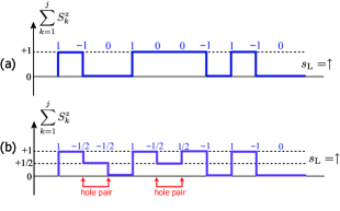
Figure 7: (Color online) Height plot of typical spin configurations in spin-1 VBS state (a) and $M=1$ sVBS state (b). Note that heights are confined within a region of width 1. Although simple ‘diluted’ Néel picture does not hold because of the presence of hole pairs, still we can find string order when hole pairs are grouped together in (b).

IV.3 String correlation

The finite-distance string correlation functiondenNijs-R-89

$$C_{\text{string}}(j;n)\equiv\Biggl{\langle}S_{j}^{z}\,\exp\left[i\pi\sum_{k=j}^{j+n-1}S^{z}_{k}\right]S^{z}_{j+n}\Biggr{\rangle}$$ (72)

can be evaluated in a similar manner. In the case of open chains, it suffers from the boundary effects. However, if we consider the case where both end points $j$ and $j+n$ are infinitely far from the chain edges, the expression simplifies a lot. In general, it contains exponentially decaying parts

$$(-1)^{n}\left\{\frac{\sqrt{8r^{2}+9}-3}{\sqrt{8r^{2}+9}+3}\right\}^{n}$$ (73)

as well as the constant (i.e. long-range-ordered) one (see Fig. 8):

$${\cal O}_{\text{string}}^{\infty}(r)=\frac{4\left\{r^{4}+14r^{2}+18+2\left(r^{2}+3\right)\sqrt{8r^{2}+9}\right\}}{\left(8r^{2}+9\right)\left(\sqrt{8r^{2}+9}+3\right)^{2}}\;.$$ (74)

Only in the limit $r\rightarrow 0$, the exponentially decaying parts disappear and the string correlation function becomes constant $4/9$ (perfect string correlation). Note that the correlation length $\xi_{\text{string}}$ is different from that ($\xi_{\text{spin}}$) for the spin-spin correlation. With increase of the hole-doping parameter $r$, the effective spin magnitude gets reduced by the increase of the spin-half sites and accordingly the string order parameter monotonically decreases (see Fig. 8).

At $r\rightarrow\infty$, the type I sVBS chain $(M=1)$ realizes the Majumdar-Ghosh dimer states with one-half spin degrees of freedom at each site and the string order parameter ${\cal O}_{\text{string}}^{\infty}$ reaches its finite minimum $1/16$, which implies that the string order survives even in the $r\nearrow\infty$ limit. This agrees with the observation that the spin-1 Haldane state is adiabatically connected to the spin-1/2 dimer stateHida-92a. Meanwhile, the type II sVBS chain $(M=1)$ is reduced to the hole-VBS chain with no spin degree of freedom at $r\rightarrow\infty$, and hence the string order vanishes completely in this limit.

In Ref. Arovas-H-Q-Z-09, a SUSY-analogue of the higher-$S$ VBS states is discussed as well. The ordinary spin-$S$ VBS states obtained in the zero hole-density ($r\rightarrow 0$) limit are known to exhibit different topological properties according to the parity of spin-$S$; the string order parameter vanishes for the even-spin VBS states while it is finite for odd-$S$Oshikawa-92; Totsuka-S-mpg-95. In this sense, it would be interesting to calculate the string order parameter ${\cal O}_{\text{string}}^{\infty}$ for the generalized sVBS states. As is seen in eq.(1), the role of spin $S$ is played by an integer $M$ (superspin) in the SUSY case. For all $M$, we can construct the matrix-product representation of the $M$-sVBS state by using $(2M+1){\times}(2M+1)$ matrices (see Appendix C) and after straightforward evaluation we obtain the results shown in Fig. 9. As is expected from the previous studies, the $r=0$ value of ${\cal O}_{\text{string}}^{\infty}$ vanishes for even-$M$. When the hole pairs are doped, on the other hand, the string order revives. In section VII, we will interpret this from the point of view of symmetry-protected topological order.

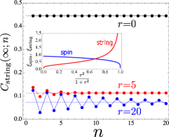
Figure 8: (Color online) String correlation function in the bulk $C_{\text{string}}(\infty;n)$ for various values of $r$: (i) $r=0$ (top; pure spin AKLT), (ii) $r=5.0$ (middle) and (iii) $r=20.0$ (bottom). Note that for the pure spin AKLT model ($r=0$), the string correlation function is constant $4/9$. For $r\neq 0$, the string correlation functions exponentially approach to the limiting values shown by dashed lines.

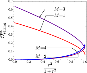
Figure 9: (Color online) The infinite-distance limit of the string correlation function ${\cal O}_{\text{string}}^{\infty}=\lim_{n\rightarrow\infty}C_{\text{string}}(\infty;n)$ for several values of $M$ plotted as a function of $r$. Note that ${\cal O}^{\infty}_{\text{string}}(r{=}0)=0$ for even-$M$ corresponding to the vanishing of string order parameter for even-$S$.

V Single-mode approximation

In this section, we consider the dynamical quantities, i.e. low-lying excitation spectra by using single-mode approximation. As is easily verified, the so-called Lieb-Schultz-Mattis twistLieb-S-M-61, which provides a basic picture of gapless low-lying excitations in half-odd-integer spin chains, does not work in the usual VBS stateTotsuka-S-mpg-95. Instead, an excited triplet bond (crackion– a ‘crack’ in a solid of valence bonds) in the valence-bond solid gives, to good approximation, a physical low-lying excitation. As has been shown by Fath and SólyomFath-S-93b, the crackions are equivalent to the triplon excitations created by spin operators $\text{\bf S}(\mathbf{k})$.

V.1 Spin excitations

Let us start by investigating the action of local spin operators

$$S^{+}_{j}=a^{\dagger}_{j}b_{j}\,,\;S^{-}_{j}=b^{\dagger}_{j}a_{j}\,,\;S^{z}_{j}=\frac{1}{2}(a^{\dagger}_{j}a_{j}-b^{\dagger}_{j}b_{j})$$ (75)

on the sVBS state. A little algebra shows that these spin operators create triplet bonds around the site $j$ (see Fig.10):

$$S^{+}_{j}|\text{sVBS-I}\rangle=|\psi^{(1)}_{j-1}\rangle-|\psi^{(1)}_{j}\rangle$$ (76a)

$$S^{z}_{j}|\text{sVBS-I}\rangle=\frac{1}{2}\left\{-|\psi^{(0)}_{j-1}\rangle+|\psi^{(0)}_{j}\rangle\right\}\;,$$ (76b)

where $|\psi^{(1)}_{j}\rangle$ and $|\psi^{(0)}_{j}\rangle$ are obtained by replacing the SUSY valence bond $(a^{\dagger}_{j}a^{\dagger}_{j+1}-b^{\dagger}_{j}b^{\dagger}_{j+1}-r\,f^{\dagger}_{j}f^{\dagger}_{j+1})$ by triplet bonds $a^{\dagger}_{j}a^{\dagger}_{j+1}$ and $(a^{\dagger}_{j}b^{\dagger}_{j+1}+b^{\dagger}_{j}a^{\dagger}_{j+1})$, respectively. This implies that the triplon-crackion equivalence holds in the sVBS case as well.

The single-mode approximation to the magnetic excitations is given by

$$\begin{split}\omega_{\text{SMA}}^{\text{s},\alpha}(k)&=-\frac{1}{2}\frac{\langle\text{sVBS-I}|\,[[{\cal H},S^{\alpha}(k)],S^{\alpha}(-k)]\,|\text{sVBS-I}\rangle}{\langle\text{sVBS-I}|S^{\alpha}(k)S^{\alpha}(-k)|\text{sVBS-I}\rangle}\\ &=\frac{\langle\text{sVBS-I}|S^{\alpha}(k){\cal H}\,S^{\alpha}(-k)|\text{sVBS-I}\rangle}{\langle\text{sVBS-I}|S^{\alpha}(k)S^{\alpha}(-k)|\text{sVBS-I}\rangle}\\ &\geq\omega_{\text{true}}^{\text{s},\alpha}(k)\;.\end{split}$$ (77)

By the SU(2) symmetry, it suffices to evaluate $\omega_{\text{SMA}}$ only for $\alpha=z$ and the spin index $\alpha$ will be suppressed hereafter. Using eq.(76b), the denominator (static structure factor) $\langle\text{sVBS-I}|S^{\alpha}(k)S^{\alpha}(-k)|\text{sVBS-I}\rangle$ is evaluated as:

$$\langle\text{sVBS-I}|S^{z}(k)S^{z}(-k)|\text{sVBS-I}\rangle\;\;(\equiv S^{zz}(k))\\ =\frac{1}{2}(1-\cos k)\langle\psi^{(0)}(k)|\psi^{(0)}(k)\rangle\;,$$ (78)

where $|\psi^{(0)}(k)\rangle$ denotes the Fourier transform

$$|\psi^{(0)}(k)\rangle=\frac{1}{\sqrt{L}}\sum_{r}\text{e}^{-ikr}|\psi^{(0)}_{r}\rangle\;.$$

Similarly, the local property of the sVBS states

$$\langle\text{sVBS-I}|h_{j,j+1}=h_{j,j+1}|\text{sVBS-I}\rangle=0\;\;(\forall j)$$ (79)

implies that only the diagonal part survives:

$$\langle\psi^{(0)}_{i}|{\cal H}|\psi^{(0)}_{j}\rangle=\delta_{i,j}\langle\psi^{(0)}_{j}|h_{j,j+1}|\psi^{(0)}_{j}\rangle\;.$$ (80)

From this, one deduces:

$$\begin{split}&\langle\text{sVBS-I}|S^{\alpha}(k){\cal H}\,S^{\alpha}(-k)|\text{sVBS-I}\rangle\\ &\quad=\frac{1}{2}(1-\cos k)\langle\psi^{(0)}_{j}|h_{j,j+1}|\psi^{(0)}_{j}\rangle\\ &\quad=\frac{1}{2}(1-\cos k)\langle\psi^{(0)}(k)|{\cal H}|\psi^{(0)}(k)\rangle\;.\end{split}$$ (81)

Eqs.(78) and (81) are combined to give

$$\begin{split}\omega^{\text{s}}_{\text{SMA}}(k)&=\frac{\langle\psi^{(0)}(k)|{\cal H}|\psi^{(0)}(k)\rangle}{\langle\psi^{(0)}(k)|\psi^{(0)}(k)\rangle}\;\;(\equiv\omega_{\text{crackion}}(k))\\ &=\frac{\langle\psi^{(0)}_{x}|h_{x,x+1}|\psi^{(0)}_{x}\rangle}{\langle\psi^{(0)}(k)|\psi^{(0)}(k)\rangle}\\ &=\frac{1}{2}\frac{(1-\cos k)}{S^{zz}(k)}\langle\psi^{(0)}_{x}|h_{x,x+1}|\psi^{(0)}_{x}\rangle\;.\end{split}$$ (82)

At this point, one may note a peculiar feature of the VBS-like states. Normally, a local excitation created by physical operators (e.g. $S^{\alpha}_{j}$) propagates on a lattice by using the off-diagonal matrix elements:

$$\langle\psi^{(0)}_{i}|{\cal H}|\psi^{(0)}_{j}\rangle\;\;(i\neq j)\;.$$ (83)

In the VBS-like models, on the other hand, $\langle\psi^{(0)}_{i}|{\cal H}|\psi^{(0)}_{j}\rangle$ is diagonal by construction (all the diagonal elements are given by $\langle\psi^{(0)}_{j}|h_{j,j+1}|\psi^{(0)}_{j}\rangle$) and excitations cannot use this channel. Rather the non-trivial $k$-dependence of $\omega_{\text{SMA}}(k)$ comes only from the non-trivial overlap between the crackion states:

$$\langle\psi^{(0)}_{i}|\psi^{(0)}_{j}\rangle=\frac{3+\sqrt{8r^{2}+9}}{2\sqrt{8r^{2}+9}}\left(-\frac{2}{3+\sqrt{8r^{2}+9}}\right)^{|i-j|}$$ (84a)

$$\left\{\langle\psi^{(0)}(k)|\psi^{(0)}(k)\rangle\right\}^{-1}\propto\frac{(1-\cos k)}{S^{zz}(k)}\;.$$ (84b)

An important conclusion can be drawn from eq.(82); the physical triplon excitation energy $\omega^{\text{s}}(k)(\leq\omega^{\text{s}}_{\text{SMA}}(k))$ becomes zero (i.e. gapless) as $k\rightarrow 0$ unless the static structure factor $S^{zz}(k)$ behaves like $k^{2}$ ($k\sim 0$). For any spin-$S$ VBS states and the sVBS states, we have checked that $S^{zz}(k)$ contains a factor $(1-\cos k)\sim k^{2}$, which opens a gap at $k=0$.

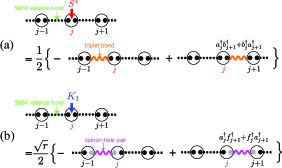
Figure 10: (Color online) Action of local spin operator $S^{z}$ (a) and fermionic generator $K_{1}$ (b) onto the sVBS state. The local operators $S^{a}_{j}$ ($a=x,y,z$) and $K_{1,2}$ respectively create a triplet bond and a spinon-hole pair (crackion) on either of the two adjacent bonds $(j-1,j)$ and $(j,j+1)$.

V.2 Hole excitations

A similar analysis can be done for the charged (hole) excitations which are always accompanied by spinon-like (i.e. $S=1/2$) objects. These excitations are created by applying the two fermionic generators of UOSp(1$|$2)

$$\begin{split}&K_{1}(j)=\frac{1}{2}(x^{-1}f_{j}a_{j}^{\dagger}+xf_{j}^{\dagger}b_{j})\\ &K_{2}(j)=\frac{1}{2}(x^{-1}f_{j}b_{j}^{\dagger}-xf_{j}^{\dagger}a_{j})\;\;(x\equiv\sqrt{r})\end{split}$$ (85)

to the VBS ground state. By using the explicit form of the ground-state wavefunction, it is easy to show

$$K_{1}(j)|\text{sVBS-I}\rangle=\frac{\sqrt{r}}{2}\left\{|\psi_{j-1}^{(1/2)}\rangle-|\psi_{j}^{(1/2)}\rangle\right\}\;,$$ (86)

where the crackion state $|\psi_{j}^{(1/2)}\rangle$ is obtained by replacing the SUSY valence bond $(a_{j}^{\dagger}b_{j+1}^{\dagger}-b_{j}^{\dagger}a_{j+1}^{\dagger}-rf_{j}^{\dagger}f_{j+1}^{\dagger})$ on the bond $(j,j+1)$ with a spinon-hole pair $(a_{j}^{\dagger}f_{j}^{\dagger}+f_{j}^{\dagger}a_{j+1}^{\dagger})$ (see Fig. 10(b)). The excited state $K_{2}|\text{sVBS}\rangle$ is defined similarly with $a^{\dagger}$ in the above expression replaced with $b^{\dagger}$. Then, the SMA excitation energy is given by an expression similar to eq.(82):

$$\begin{split}\omega^{\text{h}}_{\text{SMA}}(k)&=\frac{\langle\text{sVBS-I}|K_{1}(-k)^{\dagger}{\cal H}K_{1}(-k)|\text{sVBS-I}\rangle}{\langle\text{sVBS-I}|K_{1}(-k)^{\dagger}K_{1}(-k)|\text{sVBS-I}\rangle}\\ &=\frac{\langle\psi^{(1/2)}(j)|{\cal H}|\psi^{(1/2)}(j)\rangle}{\langle\psi^{(1/2)}(k)|\psi^{(1/2)}(k)\rangle}\;.\end{split}$$ (87)

V.3 Fixing parent Hamiltonian

Before calculating the SMA spectra (82) and (87), we have to fix the form of the parent Hamiltonian. As has been mentioned in section III, the non-hermitian parent Hamiltonian for the SUSY (UOSp($1|2$)) VBS model is givenArovas-H-Q-Z-09 by eq.(30):

$$\widetilde{\cal H}_{L=1\text{ sVBS}}=\sum_{j}\left\{V_{3/2}P_{3/2}({\cal C}_{j,j+1})+V_{2}P_{2}({\cal C}_{j,j+1})\right\}$$

with the coupling constants $V_{3/2},V_{2}\gneq 0$ positive.

The above form is not very convenient since it breaks hermiticity necessary for eq.(79) and one still has one free parameter even after the overall energy scale is fixed. Instead of using $\widetilde{\cal H}_{L=1\text{ sVBS}}$, one may adopt

$${\cal H}_{L=1\text{ sVBS}}=\widetilde{\cal H}_{L=1\text{ sVBS}}^{\dagger}\widetilde{\cal H}_{L=1\text{ sVBS}}$$ (88)

as the hermitian Hamiltonian. One way to fix the remaining coupling is to require that the SUSY parent Hamiltonian should reduce in the $r\rightarrow\infty$ to the standard (SU(2)) VBS Hamiltonianaffleck1988vbg

$${\cal H}_{S=1\text{ VBS}}=\sum_{j}\left\{\text{\bf S}_{j}{\cdot}\text{\bf S}_{j+1}+\frac{1}{3}(\text{\bf S}_{j}{\cdot}\text{\bf S}_{j+1})^{2}+\frac{2}{3}\right\}\;.$$ (89)

However, this still has a problem; since some of the matrix elements in the fermionic sector have a factor $1/r$, the limit $r\rightarrow\infty$ is divergent. Fortunately, this is not so serious. If we note that the ground states contain no fermion in the $r\rightarrow\infty$ limit, the most natural way is to require that the SUSY parent Hamiltonian projected onto the bosonic sector should coincide with the spin-1 VBS Hamiltonian (89). This fixes the two coupling constants as:

$$V_{3/2}=\tanh r\;,\;\;V_{2}=\sqrt{2}\;.$$ (90)

The spin-excitation (‘crackion’) spectrum obtained by using (82) and (90) is shown in Fig.11. At $r=0$ (AKLT-limit), the dispersion reduces to the well-known oneArovas-A-H-88:

$$\omega^{\text{s}}_{\text{SMA}}(k)=\frac{10}{27}(5+3\cos k)\;.$$ (91)

For $r\nearrow\infty$, on the other hand, the spin excitation loses the dispersion. This is easily understood since the ground-state in this limit reduces to the translationally invariant combination of two Majumdar-Ghosh states (see Fig. 1) and the overlap between crackion states, which gives the dispersion of the spin excitations, trivializes (see (82) and (84a)):

$$\langle\psi^{(0)}_{i}|\psi^{(0)}_{j}\rangle\propto\delta_{i,j}\;,\;\;\langle\psi^{(0)}(k)|\psi^{(0)}(k)\rangle=\text{const.}\;.$$ (92)

The charge excitation spectrum is calculated similarly by using eq.(87). The result is shown in Fig. 12. For $r=0$, the spectrum is given by

$$\omega_{\text{SMA}}^{\text{h}}(k)=\frac{8}{3(2-\cos k)}\;.$$ (93)

A remark is in order here about the existence of the two different spectra $\omega^{\text{s}}(k)$ and $\omega^{\text{h}}(k)$. One may naively expect $\omega^{\text{s}}(k)=\omega^{\text{h}}(k)$ as the supersymmetry relates the bosonic generators $\mathbf{S}$ and the fermionic ones $K_{\alpha}$. However, this relies on the existence of a ‘unitary’ transformation which linearly transforms the set of the SUSY generators onto themselves (adjoint representation). Since no such transformation exists here, we generally expect different spectra for the spin- and the charge sector as has been shown above.

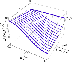
Figure 11: (Color online) The spin excitation (triplon) spectrum $\omega^{\text{s}}_{\text{SMA}}(k)$ obtained by single-mode approximation (SMA). At $r=0$, it reduces to the well-known dispersion $\omega_{\text{SMA}}(k)=10(5+3\cos k)/27$ of the spin-1 VBS model. When $r\nearrow\infty$ (Majumdar-Ghosh limit), dispersion becomes flat.

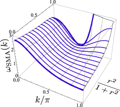
Figure 12: (Color online) The excitation spectrum $\omega^{\text{h}}_{\text{SMA}}(k)$ of a spinon-hole pair obtained by single-mode approximation (eq.(87)). This spinon-hole pair state is created by fermionic generator $K_{1}$ except at $r=0$, where the transition matrix elements of $K_{1}$ from the ground state vanish.

VI SUSY-VBS state II

Now let us add one more fermion species and consider yet another SUSY-VBS wavefunction which now includes two holes $f$ and $g$. As has been mentioned in section II.2, the state contains two (spin) bosons $(a,b)$ and two fermions $(f,g)$, and we may expect it to exhibit clearer spin-charge symmetry with respect to $r=1$.

The second generalized sVBS wavefunction (the case $M=1$ of eq.(13)) is defined by:

$$\begin{split}&|\text{sVBS-II}\rangle\\ &\equiv(\cdots)\left\{a^{\dagger}_{j-1}b^{\dagger}_{j}-b^{\dagger}_{j-1}a^{\dagger}_{j}-r(f^{\dagger}_{j-1}g^{\dagger}_{j}+g^{\dagger}_{j-1}f^{\dagger}_{j})\right\}\\ &\quad\left\{a^{\dagger}_{j}b^{\dagger}_{j+1}-b^{\dagger}_{j}a^{\dagger}_{j+1}-r(f^{\dagger}_{j}g^{\dagger}_{j+1}+g^{\dagger}_{j}f^{\dagger}_{j+1})\right\}(\cdots)|0\rangle\;.\end{split}$$ (94)

As we have seen in section II.2, this state is based on the algebra UOSp(2$|$2) and one can construct the parent Hamiltonian in a similar manner to the type I case (based on UOSp(1$|$2)) (we do not give the explicit form here. The interested readers may refer the online supplementary materialsupp.).

VI.1 Matrix-product representation

We follow the same steps as in section III with a different metric matrix

$${\cal R}_{\text{II}}=\begin{pmatrix}0&1&0&0\\ -1&0&0&0\\ 0&0&0&-1\\ 0&0&-1&0\end{pmatrix}$$ (95)

and the spinor $(a^{\dagger}_{j},b^{\dagger}_{j},\sqrt{r}f^{\dagger}_{j},\sqrt{r}g^{\dagger}_{j})^{\text{t}}$ to obtain the MPS representation for the second sVBS state:

$$\begin{split}A_{j}&=\begin{pmatrix}b^{\dagger}_{j}\\ -a^{\dagger}_{j}\\ -\sqrt{r}g^{\dagger}_{j}\\ -\sqrt{r}f^{\dagger}_{j}\end{pmatrix}\begin{pmatrix}a^{\dagger}_{j}&b^{\dagger}_{j}&\sqrt{r}f^{\dagger}_{j}&\sqrt{r}g^{\dagger}_{j}\end{pmatrix}|\text{vac}\rangle_{j}\\ &=\begin{pmatrix}a^{\dagger}_{j}b^{\dagger}_{j}&(b^{\dagger}_{j})^{2}&\sqrt{r}b^{\dagger}_{j}f^{\dagger}_{j}&\sqrt{r}b^{\dagger}_{j}g^{\dagger}_{j}\\ -(a^{\dagger}_{j})^{2}&-a^{\dagger}_{j}b^{\dagger}_{j}&-\sqrt{r}a^{\dagger}_{j}f^{\dagger}_{j}&-\sqrt{r}a^{\dagger}_{j}g^{\dagger}_{j}\\ -\sqrt{r}g^{\dagger}_{j}a^{\dagger}_{j}&-\sqrt{r}g^{\dagger}_{j}b^{\dagger}_{j}&-rg^{\dagger}_{j}f^{\dagger}_{j}&0\\ -\sqrt{r}f^{\dagger}_{j}a^{\dagger}_{j}&-\sqrt{r}f^{\dagger}_{j}b^{\dagger}_{j}&0&-rf^{\dagger}_{j}g^{\dagger}_{j}\end{pmatrix}|\text{vac}\rangle_{j}\end{split}$$ (96a)

$$\begin{split}A^{\dagger}_{j}&={}_{j}\langle\text{vac}|\begin{pmatrix}a_{j}\\ b_{j}\\ \sqrt{r}f_{j}\\ \sqrt{r}g_{j}\end{pmatrix}\begin{pmatrix}b_{j}&-a_{j}&-\sqrt{r}g_{j}&-\sqrt{r}f_{j}\end{pmatrix}\\ &={}_{j}\langle\text{vac}|\begin{pmatrix}a_{j}b_{j}&-(a_{j})^{2}&-\sqrt{r}a_{j}g_{j}&-\sqrt{r}a_{j}f_{j}\\ (b_{j})^{2}&-a_{j}b_{j}&-\sqrt{r}b_{j}g_{j}&-\sqrt{r}b_{j}f_{j}\\ \sqrt{r}f_{j}b_{j}&-\sqrt{r}f_{j}a_{j}&-rf_{j}g_{j}&0\\ \sqrt{r}g_{j}b_{j}&-\sqrt{r}g_{j}a_{j}&0&-rg_{j}f_{j}\end{pmatrix}\end{split}$$ (96b)

As in the first sVBS state, the supertrace is necessary for the periodic system:

$$|\text{sVBS-II}\rangle=\text{STr}\left\{\bigotimes_{j=1}^{L}A_{j}\right\}\;,$$ (97)

where $\text{STr}(\mathcal{M})\equiv\mathcal{M}_{11}+\mathcal{M}_{22}-\mathcal{M}_{33}-\mathcal{M}_{44}$. The $T$-matrix is a 16$\times$16 matrix and has seven different eigenvalues $\lambda_{i}$ (see Fig. 13):

$$\begin{split}\{\lambda_{i}\}=&\bigl{\{}-1(\times 3),-ir(\times 4),+ir(\times 4),-r^{2}(\times 2),r^{2},\\ &\frac{1}{2}\left(r^{2}+3-f(r)\right),\frac{1}{2}\left(r^{2}+3+f(r)\right)\bigr{\}}\;,\end{split}$$ (98)

where $f(r)\equiv\sqrt{r^{4}+10r^{2}+9}$. Regardless of the value of $r$, the eigenvalue with largest modulus is:

$$\lambda_{1}=\frac{1}{2}\left(r^{2}+3+f(r)\right)\;.$$ (99)

Since the set of eigenvalues is invariant under $r\leftrightarrow-r$, we can restrict ourselves to $r\geq 0$.

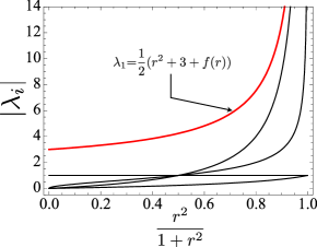
Figure 13: (color online) Plot of absolute values $|\lambda_{i}|$ of the seven different eigenvalues of $G$. Since $|\lambda_{i}|$s are symmetric with respect to $r\mapsto-r$, only the $r>0$ part is shown.

VI.2 spin-spin correlation

Let us begin with the spin-spin correlation function. By using the method described in Appendix B.2, it is straightforward to calculate the correlation function $\langle S^{a}_{j}S^{a}_{j+n}\rangle$:

$$\begin{split}&\langle S^{a}_{j}S^{a}_{j+n}\rangle\\ &=\begin{cases}\frac{2}{f(r)}&\;\text{for }n=0\\ \frac{r^{2}+5+f(r)}{2f(r)}\left(-\frac{2}{r^{2}+3+f(r)}\right)^{n}&\;\text{for }n>0\;.\end{cases}\end{split}$$ (100)

In obtaining these expressions, it has been assumed that both end points ($x$ and $x+n$) are infinitely far from the edges (otherwise there will be another decaying factor coming from the edge effects). From these, we can read off the spin-spin correlation length:

$$\xi_{\text{spin}}(r)=1/\log\left\{\left(r^{2}+3+f(r)\right)/2\right\}\;,$$ (101)

which monotonically decreases from $1/\ln(3)$ ($r=0$) to 0 ($r\nearrow\infty$).

The existence of the edge states may be best illustrated by plotting the local magnetization $\langle S^{z}_{j}\rangle$.

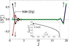
Figure 14: (color online) Plot of local magnetization profile $\langle S^{z}_{j}\rangle$ for different (left) edge states (with right edge fixed). (inset) Spin correlation length $\xi_{\text{spin}}(r)$ as a function of $r$. It monotonically decreases as $r$ is increased and approaches to zero like $\xi_{\text{spin}}\sim 1/\log\left(1+r^{2}\right)$.

VI.3 Superconducting correlation

Since the type-II sVBS state (13) contains hole pairs on adjacent sites, we may expect that the pair amplitudes take finite expectation values. As in section III.4, we may define the following order parameters on general grounds:

$$\Delta^{ff}_{j} \equiv(a_{j}b_{j+1}-b_{j}a_{j+1})f^{\dagger}_{j}f^{\dagger}_{j+1}$$ (102a)

$$\Delta^{gg}_{j} \equiv(a_{j}b_{j+1}-b_{j}a_{j+1})g^{\dagger}_{j}g^{\dagger}_{j+1}$$ (102b)

$$\Delta^{fg}_{j} \equiv(a_{j}b_{j+1}-b_{j}a_{j+1})(f^{\dagger}_{j}g^{\dagger}_{j+1}+g^{\dagger}_{j}f^{\dagger}_{j+1})\;.$$ (102c)

However, the first two are identically zero by construction of $|\text{sVBS-II}\rangle$. The only non-vanishing superconducting order parameter

$${\cal O}_{\text{sc}}=\langle\Delta^{fg}_{j}\rangle$$ (103)

is plotted in Fig. 15 for various values of $r$. Also plotted are the hole ($f$ and $g$) number $\langle n_{f,g}\rangle$ and the hole-number fluctuation $\delta n_{\text{hole}}$:

$$\begin{split}&\langle n_{f}\rangle=\langle f_{j}^{\dagger}f_{j}\rangle=\langle g^{\dagger}_{j}g_{j}\rangle=\langle n_{g}\rangle\,,\\ &\delta n_{\text{hole}}=\langle n^{2}_{\text{hole}}\rangle-\langle n_{\text{hole}}\rangle^{2}\;(n_{\text{hole}}\equiv n_{f}+n_{g})\;.\end{split}$$ (104)

The superconducting order parameter ${\cal O}_{\text{SC}}$ is maximal at $r\approx 1.05$ (or, $r^{2}/(1+r^{2})\approx 0.52$).

The superconducting correlation (hole-hole correlation)

$$C^{fg}_{\text{sc}}(n)\equiv(a_{j}b_{j+n}-b_{j}a_{j+n})(f^{\dagger}_{j}g^{\dagger}_{j+n}+g^{\dagger}_{j}f^{\dagger}_{j+n})$$ (105)

decays exponentially with the correlation length

$$\xi_{\text{sc}}(r)=\log^{-1}\left\{\frac{r^{2}+3+f(r)}{2r}\right\}\;.$$ (106)

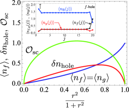
Figure 15: (Color online) Plot of ${\cal O}_{\text{sc}}=\langle\Delta_{j}\rangle$, the hole density $\langle n_{\text{hole}}(j)\rangle=\langle f^{\dagger}_{j}f_{j}\rangle$ and the hole-number fluctuation $\langle f^{\dagger}_{j}f_{j}\rangle-\langle f^{\dagger}_{j}f_{j}\rangle^{2}$ as a function of $r$. Here the bulk values are plotted. (Inset): Profile of the hole density ($r=0.5$ or $r^{2}/(1+r^{2})=0.2$) for a finite system ($L=20$). Only the left edge state is changed with the right one fixed to $s_{\text{R}}=\uparrow$. The hole density approaches exponentially to the bulk value as we move away from the edge.

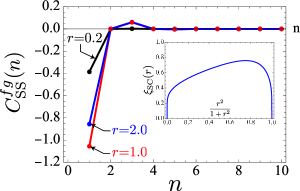
Figure 16: (Color online) Plot of hole correlation $C^{fg}_{\text{SC}}(n)=(a_{j}b_{j+n}-b_{j}a_{j+n})(f^{\dagger}_{j}g^{\dagger}_{j+n}+g^{\dagger}_{j}f^{\dagger}_{j+n})$ for various $r$. Due to the form of the wave function, hole correlation identically vanishes when the distance $n$ is even. Inset: correlation length $\xi_{\text{SC}}(r)$ of the hole correlation.

VI.4 String correlation

Then, we proceed to the string correlation function. As in the previous case (type I sVBS), the string correlation explicitly depends on the distance between the two end points through the exponentially decaying factor:

$$(-1)^{n}\left\{\frac{f(r)-(r^{2}+3)}{f(r)+(r^{2}+3)}\right\}^{n}\;.$$ (107)

These expressions imply that the correlation lengths ($\xi_{\text{string}}$) for the string correlation are different from $\xi_{\text{spin}}$ for the spin-spin correlation function.

The infinite-distance limit of the string correlation is given as:

$${\cal O}^{\infty}_{\text{string}}=\frac{4}{\left(r^{2}+1\right)\left(r^{2}+9\right)}\;.$$ (108)

It is easy to check that when $r=0$ eq.(108) reproduces the value $4/9$ of the spin-1 AKLT modelKennedy-T-92a. The results are plotted in Fig. 17 together with the correlation length $\xi_{\text{string}}(r)$. In contrast to the first case $|\text{sVBS-I}\rangle$ (see Fig. 9), the $r\nearrow\infty$ limit of ${\cal O}_{\text{string}}^{\infty}$ is zero since spins disappear from the state $|\text{sVBS-II}\rangle$ in this limit.

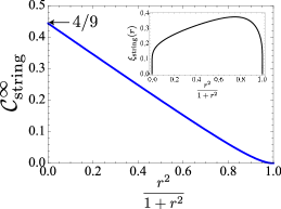
Figure 17: The infinite-distance limit of the string correlation function $\langle S_{x}^{z}\exp[i\pi\sum_{j=x}^{x+n-1}S_{j}^{z}]S^{z}_{x+n}\rangle$ ($n\nearrow\infty$) as a function of $r$. The value of string correlation smoothly decreases from the AKLT value $4/9$ to 0 (no spins left).

VII Symmetry-protected topological order

Though the string-order parameter captures the diluted Néel order of the Haldane phase, the string-order itself is fragile under small perturbations Anfuso-R-07-2; Gu-W-09. Recently, Li and Haldane proposed Li-H-08 to use the structure of the low-lying part of the entanglement spectrum (the logarithm of the eigenvalues of the reduced density matrix for either of the two partitioned systems) as the signature of topological order inherent in the state. Pollmann et al. Pollmann-T-B-O-10; pollmann-2009 have investigated the relation between the level structure (e.g. degeneracy) of the entanglement spectrum and discrete symmetries of the system; they showed that, for odd-$S$ spin chains, the existence of (at least one of) the three discrete symmetries (time-reversal symmetry, link-inversion, and $\mathbb{Z}_{2}\times\mathbb{Z}_{2}$ symmetry) guarantees (at least two-fold) degeneracy in each entanglement level, while for even-$S$ spin chains, the existence of the above discrete symmetries tells nothing about degeneracy. By this observation, they have argued that the Haldane phase in odd-$S$ spin chains is a stable topological phase protected by discrete symmetries.

Such arguments can also be applicable to the stability discussion of the Haldane-like phase of the present SUSY spin models. For instance, the type I sVBS states contains the UOSp(1$|$2) superspin-$M$ multiplet that consists of two SU(2) spin multiplets whose spins differ by $1/2$. By partitioning a superspin-$M$ sVBS infinite chain to two semi-infinite segments, there appear two SU(2) spins $M/2$ and $(M-1)/2$ on the “edge” of each of two sVBS chain segments (hence $(2M+1)$ edge states instead of $(S+1)$ ones in the usual spin-$S$ VBS states). It is noted that, regardless of the parity of the bulk superspin $M$, the sVBS state accommodates a half-integer SU(2) spin on the edge. Therefore, for any integer-superspin sVBS states, the entanglement spectrum always contains a sector consisting of at least doubly degenerate levels which come from the half-integer SU(2) spin sector of the entanglement Hilbert space. For example, the entanglement spectrum of the $M=2$ sVBS state consists of a doubly degenerate level corresponding to the doubly degenerate fermionic sector and a bosonic level with three-fold degeneracy. In fact, we can show that if one of the discrete symmetries (link inversion and time-reversal) is present in the SUSY spin chains, there is always a sector in the entanglement spectrum each of whose levels is at least doubly degenerate. This implies that the ‘Haldane phase’ is stabilized regardless of the parity of the bulk (integer) superspins. We will report the details elsewhere.

VIII Summary

In the present paper, we have constructed a supersymmetric extension of the matrix-product states (sMPS) for two different types (I and II) of supersymmetric VBS (sVBS) states and exactly evaluated various physical quantities. The sMPS constructed here contains the fermionic elements as well as the usual bosonic (i.e. commuting) ones and this slightly complicates the treatment (for instance, instead of the trace, the supertrace is used for the periodic systems). We investigated the hole-doping behaviors of various correlation functions (spin-spin and superconducting) and the spin- and the hole excitation spectrum.

In the charge sector, the type I sVBS chains exhibit insulating behavior at zero and infinite concentrations of the doped holes and the superconducting order parameter is finite only for finite doping. In the spin sector, the type I sVBS chains interpolate between the usual VBS state and the inhomogeneous VBS state (in the simplest case, it reduces to the MG dimer state) at the two extremal limits of hole-doping $r=0$ and $r=\infty$, respectively. The single-mode approximation has been applied to obtain the spin- and the charge excitation spectrum. There are two types of low-lying excitations, $i.e.$ the triplon and the spinon-hole pair, created respectively by the bosonic and fermionic generators of the super Lie algebra. The spinon-hole pair is peculiar to the sVBS states; it simultaneously possesses the property of the spin-$1/2$ spinon and the unpaired hole in the superconducting background. We have found that the spinon-hole pair can be the lowest excitation in some parameter region of the hole-doping.

As another class of sVBS states based on a larger ($\mathcal{N}{=}2$) SUSY, we have introduced the type II sVBS states. In the high-doping limit ($r\rightarrow\infty$), the superspin-1 ($M=1$) type II sVBS state reduces to the totally uncorrelated hole-VBS state, while it reproduces the spin VBS state in the zero-doping limit. The type II sVBS state displays qualitatively similar behaviors in the spin- and the charge properties except that now physical quantities are more symmetric with respect to the point $r=1$ reflecting that the model contains the equal numbers of bosons and fermions.

We have demonstrated the existence of a hidden order in the sVBS states (both type I and II) by calculating the non-local string correlations. What is remarkable is that the string correlation revives upon hole doping although it vanishes in the pure-spin limit $r\rightarrow 0$ when the spin $S=M$ is even integer. This may be understood as an example of symmetry-protected topological order in SUSY spin chains.

Though the present work is restricted to 1D chains, the sVBS states themselves can be formulated on any lattice in arbitrary dimensions, and may generally exhibit resonating-valence-bond (RVB) features at finite hole doping. For instance, an $M=2$ sVBS state with three species of holes simulates the Rokhsar-Kivelson RVBRokhsar-K-88 in the high-doping limit. Such higher dimensional analyses are interesting both theoretically and experimentally, and may be carried by a supersymmetric extension of the tensor network method.

Appendix A A crash course on supersymmetry

A.1 UOSp(1$|$2) and UOSp(2$|$2)

The superalgebra UOSP(1$|$2) consists of the following five generators

$$\begin{split}&S^{x}=(a^{\dagger}b+b^{\dagger}a)/2\;,\;S^{y}=(a^{\dagger}b-b^{\dagger}a)/(2i),\\ &S^{z}=(a^{\dagger}a-b^{\dagger}b)/2\;\;(\text{bosonic})\end{split}$$ (109a)

$$\begin{split}&K_{1}=\frac{1}{2}(x^{-1}fa^{\dagger}+xf^{\dagger}b)\\ &K_{2}=\frac{1}{2}(x^{-1}fb^{\dagger}-xf^{\dagger}a)\;\;(\text{fermionic})\end{split}$$ (109b)

satisfying the (anti)commutation relations:

$$\begin{split}&[S^{a}\,,\,S^{b}]=i\epsilon^{abc}S^{c}\quad(a,b,c=x,y,z)\\ &[S^{a}\,,\,K_{\mu}]=\frac{1}{2}K_{\nu}(\sigma^{a})_{\nu\mu}\quad(\mu,\nu=1,2)\\ &\{K_{\mu}\,,\,K_{\nu}\}=\frac{1}{2}(i\sigma^{y}\sigma^{a})_{\mu\nu}S^{a}\;.\end{split}$$ (109c)

At this stage, the parameter $x$, which defines a one-parameter deformation of UOSp(1$|$2), is arbitrary. The second equation implies that the fermionic generators $K_{1}$ and $K_{2}$ span a two-dimensional spinor representation of SU(2).

Any irreducible representation of UOSp(1$|$2) is specified by superspin $l(=0,1/2,1,\ldots)$. A convenient way of constructing a superspin-$l$ representation is to use Schwinger operators (bosons $a$, $b$ and fermion $f$) satisfying

$$n_{a}+n_{b}+n_{f}\equiv a^{\dagger}a+b^{\dagger}b+f^{\dagger}f=2l\;(\in\mathbb{Z})\;.$$ (110)

Then, the Casimir operator ${\cal C}$ is calculated as:

$${\cal C}\equiv\text{\bf S}^{2}+(K_{1}K_{2}-K_{2}K_{1})=l(l+1/2)\;.$$ (111)

The SU(2) subalgebra depends only on $a$ and $b$:

$$\begin{split}&\text{\bf S}^{2}=\left\{(n_{a}+n_{b})^{2}+2(n_{a}+n_{b})\right\}/4=S(S+1)\\ &S=(n_{a}+n_{b})/2\;.\end{split}$$ (112)

Since $n_{f}=0,1$, a $(4l{+}1)$-dimensional superspin-$l$ representation splits into two SU(2) irreducible representations:

$$\begin{split}&\text{(i)}\;S=l\;\;(n_{f}=0)\cdots(2l+1)\text{-dim}\\ &\text{(ii)}\;S=l-1/2\;\;(n_{f}=1)\cdots 2l\text{-dim}\;,\end{split}$$ (113)

which are connected to each other by the fermionic generators $K_{1,2}$. For instance, the five states in the $l=1$ representation are:

$$\begin{split}&\text{(i)}\;|+\rangle=\frac{1}{2}{a_{i}^{\dagger}}^{2}|\text{vac}\rangle,\quad|0\rangle={a_{i}^{\dagger}b_{i}^{\dagger}}|\text{vac}\rangle,\quad|-\rangle=\frac{1}{2}{b_{i}^{\dagger}}^{2}|\text{vac}\rangle,\\ &\text{(ii)}\;|\!\uparrow\rangle=a_{i}^{\dagger}f_{i}^{\dagger}|\text{vac}\rangle,\quad|\!\downarrow\rangle=b_{i}^{\dagger}f_{i}^{\dagger}|\text{vac}\rangle\;.\end{split}$$ (114)

In constructing the sVBS states, we identify (ii) as a one-hole state. The $l=1/2$ case is relevant in realizing the so-called superqubitborsten-2010-81.

A two-site system can be treated in the same manner as in SU(2); we just define $\text{\bf S}^{\text{tot}}=\text{\bf S}^{(1)}+\text{\bf S}^{(2)}$, $K_{1,2}^{\text{tot}}=K_{1,2}^{(1)}+K_{1,2}^{(2)}$ and the corresponding Casimir operator by

$$\begin{split}{\cal C}_{1,2}&\equiv\text{\bf S}^{\text{tot}}{\cdot}\text{\bf S}^{\text{tot}}+\epsilon_{\mu\nu}K^{\text{tot}}_{\mu}K^{\text{tot}}_{\nu}\\ &={\cal C}^{(1)}+{\cal C}^{(2)}+2\left\{\text{\bf S}^{(1)}{\cdot}\text{\bf S}^{(2)}+\epsilon_{\mu\nu}K_{\mu}^{(1)}K_{\nu}^{(2)}\right\}\\ &\equiv{\cal C}^{(1)}+{\cal C}^{(2)}+2{\cal S}^{(1)}{\cdot}{\cal S}^{(2)}\;.\end{split}$$ (115)

The Clebsch-Gordan decomposition is simply given as:

$$l\otimes l\simeq 0\oplus\frac{1}{2}\oplus 1\oplus\cdots\oplus(2l-1/2)\oplus 2l\;.$$ (116)

So far, the deformation parameter $x$ is arbitrary. However, in order for $(a_{1}^{\dagger}b^{\dagger}_{2}-b_{1}^{\dagger}a^{\dagger}_{2}-rf_{1}^{\dagger}f^{\dagger}_{2})$ to behave as a UOSp(1$|$2)-singlet, $x^{2}=r$ is required.

By flipping the relative signs of the first and second terms in $K_{\mu}$ (109b), one may define “new” fermionic operators:

$$D_{1}=\frac{1}{2}(-x^{-1}fa^{\dagger}+xf^{\dagger}b)$$

$$D_{2}=-\frac{1}{2}(x^{-1}fb^{\dagger}+xf^{\dagger}a).$$ (117)

The type I sVBS states are not invariant under the transformation generated by $D_{\mu}$. (Thus, the largest symmetry of the type I sVBS states is UOSp(1$|$2).) With inclusion of $D_{\mu}$, the UOSp(1$|$2) generators satisfy the UOSp(2$|$2) algebra

$$\begin{split}&[S_{a},S_{b}]=i\epsilon_{abc}S_{c}\,,\;\;\{K_{\mu},K_{\nu}\}=\frac{1}{2}(\epsilon\sigma_{a})_{\mu\nu}S_{a}\,,\\ &\{D_{\mu},D_{\nu}\}=-\frac{1}{2}{(\epsilon\sigma_{a})}_{\mu\nu}S_{a}\,,\\ &[S_{a},K_{\mu}]=\frac{1}{2}(\sigma_{a})_{\nu\mu}K_{\nu}\,,\;\;[S_{a},D_{\mu}]=\frac{1}{2}(\sigma_{a})_{\nu\mu}D_{\nu}\,,\\ &\{K_{\mu},D_{\nu}\}=-{\frac{1}{4}}\epsilon_{\mu\nu}\Gamma\,,\\ &[S_{a},\Gamma]=0\,,\;\;[K_{\mu},\Gamma]=-D_{\mu}\,,\;\;[D_{\mu},\Gamma]=-K_{\mu}\,,\end{split}$$ (118)

where $\Gamma$ is defined by

$$\Gamma=a^{\dagger}a+b^{\dagger}b+2f^{\dagger}f\;.$$ (119)

Appendix B A quick recipe for matrix-formalism

In this section, we extend the standard formalism for bosonic matrix-product states so that we can handle fermionic states as well.

B.1 Norm

We begin with the computation of the norm of $|\text{MPS}\rangle$. Since we consider cases where $A_{j}$ is made up with both bosonic- and fermionic states, a special care has to be taken and we proceed step by step. If we write the matrix indicies explicitly, $|\text{MPS}\rangle$ reads:

$$\begin{split}&|\text{MPS}\rangle_{(\alpha,\gamma)}\\ &=\sum_{\{\beta_{j}\}}A_{1}(\alpha,\beta_{1})A_{2}(\beta_{1},\beta_{2})\dots\\ &\phantom{\sum_{\{\beta_{j}\}}}\underrightarrow{\dots A_{j}(\beta_{j-1},\beta_{j})A_{j+1}(\beta_{j},\beta_{j+1})\dots}A_{L}(\beta_{L-1},\gamma)\;,\end{split}$$ (120)

where the arrow indicates how the order of matrix multiplication and the site indices ($1,2,\ldots,l$) are related. If the parent Hamiltonian ${\cal H}=\sum_{j}h_{j,j+1}$ is defined in such a way that

$$h_{j,j+1}(A_{j}\otimes A_{j+1})=0\;\;\text{(for all matrix elements)}\;,$$ (121)

the matrix indices are physically related to some zero-energy degrees of freedom localized at the boundaries (edge states). It is important to keep the order ($\rightarrow$) of the string of matrices. If we adopt the following convention for the hermitian conjugation of fermionic operators:

$$\left(f_{1}f_{2}\dots f_{i-1}f_{i}\right)^{\dagger}\equiv f^{\dagger}_{i}f^{\dagger}_{i-1}\dots f^{\dagger}_{2}f^{\dagger}_{1}\;,$$ (122)

then the dual of $|\text{MPS}\rangle$ reads

$$\begin{split}&\langle\text{MPS}|_{(\alpha,\gamma)}\\ &=\sum_{\{\bar{\beta}_{j}\}}A^{\ast}_{L}(\bar{\beta}_{L-1},\gamma)\dots\\ &\qquad A^{\ast}_{j+1}(\bar{\beta}_{j},\bar{\beta}_{j+1})A^{\ast}_{j}(\bar{\beta}_{j-1},\bar{\beta}_{j})\dots A^{\ast}_{2}(\bar{\beta}_{1},\bar{\beta}_{2})A^{\ast}_{1}(\alpha,\bar{\beta}_{1})\\ &=\sum_{\{\bar{\beta}_{j}\}}A^{\dagger}_{L}(\gamma,\bar{\beta}_{L-1})\dots\\ &\qquad\underleftarrow{A^{\dagger}_{j+1}(\bar{\beta}_{j+1},\bar{\beta}_{j})A^{\dagger}_{j}(\bar{\beta}_{j},\bar{\beta}_{j-1})\dots}A^{\dagger}_{2}(\bar{\beta}_{2},\bar{\beta}_{1})A^{\dagger}_{1}(\bar{\beta}_{1},\alpha)\;,\end{split}$$ (123)

where $A^{\ast}_{j}$ and $A^{\dagger}_{j}$ denotes a matrix obtained by replacing $|\cdot\rangle\mapsto\langle\cdot|$ in $A_{j}$ and its transposition.

For a periodic chain, the fermion sign has to be treated carefully. Using the identity $\psi_{L}^{t}\mathcal{R}\psi_{1}=\text{STr}(\mathcal{R}\psi_{1}\psi_{L}^{t})$ (the supertrace STr is defined in such a way that extra minus signs are multiplied for the fermionic sectors. See (42b) and (97), for instance), we can express the supersymmetric MPS (sMPS) as

$$\begin{split}|\text{sMPS}\rangle_{\text{PBC}}&=\underbrace{\prod_{i=1}^{L-1}(\psi_{i}^{t}\mathcal{R}\psi_{i+1})}_{\text{Grassmann even}}\psi^{\alpha}_{L}({\cal R}\psi_{1})^{\alpha}|0\rangle\\ &=\text{STr}\left\{({\cal R}\psi_{1})\prod_{i=1}^{L-1}(\psi_{i}^{t}\mathcal{R}\psi_{i+1})\psi_{L}^{t}\right\}\\ &=\text{STr}(A_{1}A_{2}\cdots A_{L}).\end{split}$$ (124)

Since the overlap $A_{j}^{\ast}(\bar{\beta}_{j-1},\bar{\beta}_{j})A_{j}(\beta_{j-1},\beta_{j})$ is a commuting $c$-number (transfer matrix), it is straightforward to show, by proceeding term by term from the inner most overlap to the outer, the following equation:

$$\langle\text{MPS}|\text{MPS}\rangle_{(\alpha,\gamma)}=\{T_{1}\cdots T_{j}\cdots T_{L}\}_{(\alpha,\alpha;\gamma,\gamma)}\;,$$ (125a)

where

$$\begin{split}&T_{1}(\alpha,\alpha;\bar{\beta}_{1},\beta_{1})\equiv A_{1}^{\ast}(\alpha,\bar{\beta}_{1})A_{1}(\alpha,\beta_{1})\\ &T_{L}(\bar{\beta}_{L-1},\beta_{L-1};\bar{\gamma},\gamma)\equiv A_{L}^{\ast}(\bar{\beta}_{L-1},\bar{\gamma})A_{L}(\beta_{L-1},\gamma)\\ &T_{j}(\bar{\beta}_{j-1},\beta_{j-1};\bar{\beta}_{j},\beta_{j})\equiv A_{j}^{\ast}(\bar{\beta}_{j-1},\bar{\beta}_{j})A_{j}(\beta_{j-1},\beta_{j})\;.\end{split}$$ (125b)

For the purpose of calculating various correlation functions, it is convenient to consider generalized overlaps of the following form:

$$\begin{split}{}_{(\alpha,\beta)}\langle\text{MPS}|\text{MPS}\rangle_{(\gamma,\delta)}&=\{T_{1}\cdots T_{j}\cdots T_{L}\}_{(\alpha,\gamma;\beta,\delta)}\\ &=\{T^{L}\}_{(\alpha,\gamma;\beta,\delta)}\;,\end{split}$$ (126)

which are not necessarily proportional to $\delta_{\alpha,\gamma}\delta_{\beta,\delta}$ for finite-$L$. If the periodic boundary condition is imposed, the norm corresponding to the bosonic MPS eq.(32b) reads

$$\langle\text{MPS}|\text{MPS}\rangle_{\text{PBC}}=\sum_{\alpha,\beta}\left\{T^{L}\right\}_{(\alpha,\beta;\alpha,\beta)}=\text{Tr}\,T^{L}\;.$$ (127)

In the case of sMPS, the above expression should be replaced with eq.(46a).

B.2 Correlation functions

Having established the way of evaluating overlaps, it is straightforward to extend it to correlation functions. For simplicity, we only consider bosonic operators here (we will generalize the calculation to fermionic operators as well).

Let us consider first the ordinary two-point correlation function:

$$\langle{\cal O}^{A}_{x}{\cal O}^{B}_{y}\rangle_{(\alpha,\gamma)}=\frac{\langle\text{MPS}|{\cal O}^{A}_{x}{\cal O}^{B}_{y}|\text{MPS}\rangle_{(\alpha,\gamma)}}{\langle\text{MPS}|\text{MPS}\rangle_{(\alpha,\gamma)}}\;.$$ (128)

Since the two physical operators ${\cal O}^{A}_{x}$ and ${\cal O}^{B}_{y}$ are bosonic, the calculation goes in almost the same manner as in the case of norms except that here we have two new matrices:

$$\begin{split}&T^{{\cal O}^{A}}_{x}(\bar{\beta}_{x-1},\beta_{x-1};\bar{\beta}_{x},\beta_{x})\equiv A_{x}^{\ast}(\bar{\beta}_{x-1},\bar{\beta}_{x}){\cal O}^{A}_{x}A_{x}(\beta_{x-1},\beta_{x})\\ &T^{{\cal O}^{B}}_{y}(\bar{\beta}_{y-1},\beta_{y-1};\bar{\beta}_{y},\beta_{y})\equiv A_{y}^{\ast}(\bar{\beta}_{y-1},\bar{\beta}_{y}){\cal O}^{B}_{y}A_{y}(\beta_{y-1},\beta_{y})\end{split}$$ (129)

instead of $T_{x}$ and $T_{y}$. Then, by using (126), the numerator of eq.(128) may be expressed as:

$$\left\{T^{x-1}T^{{\cal O}^{A}}T^{y-x-1}T^{{\cal O}^{B}}T^{L-y}\right\}_{(\alpha,\alpha;\gamma,\gamma)}\;.$$ (130a)

Therefore, the matrix-product expression of the correlation function is given by:

$$\langle{\cal O}^{A}_{x}{\cal O}^{B}_{y}\rangle_{(\alpha,\gamma)}=\frac{\left\{T^{x-1}T^{{\cal O}^{A}}T^{y-x-1}T^{{\cal O}^{B}}T^{L-y}\right\}_{(\alpha,\alpha;\gamma,\gamma)}}{\left\{\widetilde{T}T^{L-1}\right\}_{(\alpha,\alpha;\gamma,\gamma)}}\;.$$ (130b)

In physical applications, we will encounter the following string-like correlation functions:

$$\Biggl{\langle}{\cal O}^{A}_{x}\left(\prod_{j=x+1}^{y-1}{\cal O}^{C_{j}}_{j}\right){\cal O}^{B}_{y}\Biggr{\rangle}_{(\alpha,\gamma)}\\ =\frac{\langle\text{MPS}|{\cal O}^{A}_{x}\left(\prod_{j=x+1}^{y-1}{\cal O}^{C_{j}}_{j}\right){\cal O}^{B}_{y}|\text{MPS}\rangle_{(\alpha,\gamma)}}{\langle\text{MPS}|\text{MPS}\rangle_{(\alpha,\gamma)}}\;.$$ (131a)

It is straightforward to obtain:

$$\begin{split}&\Biggl{\langle}{\cal O}^{A}_{x}\left(\prod_{j=x+1}^{y-1}{\cal O}^{C_{j}}_{j}\right){\cal O}^{B}_{y}\Biggr{\rangle}_{(\alpha,\gamma)}\\ &=\frac{\left\{T^{x-1}T^{{\cal O}^{A}}(T^{{\cal O}^{C}})^{y-x-1}T^{{\cal O}^{B}}T^{L-y}\right\}_{(\alpha,\alpha;\gamma,\gamma)}}{\left\{T^{L}\right\}_{(\alpha,\alpha;\gamma,\gamma)}}\;.\end{split}$$ (131b)

In order to calculate the so-called string correlation function (see section IV), we should take:

$${\cal O}^{A}=S^{x,z}\text{e}^{i\pi S^{x,z}}\;,\;\;{\cal O}^{B}=S^{x,z}\;,\;\;{\cal O}^{C}=\text{e}^{i\pi S^{x,z}}\;.$$ (132)

When we consider the expectation values involving fermionic operators, the calculation is slightly more complicated as we have seen in section III.4.

Appendix C MPS for Type I sVBS with general $M$

The construction of MPS for the $M=1$ type-I VBS state in section III.1 can be readily generalized to general $M$. To this end, it is helpful to note that

$$(a^{\dagger}_{j}b^{\dagger}_{j+1}-b^{\dagger}_{j}a^{\dagger}_{j+1}-rf^{\dagger}_{j}f^{\dagger}_{j+1})^{M}\\ =(a^{\dagger}_{j}b^{\dagger}_{j+1}-b^{\dagger}_{j}a^{\dagger}_{j+1})^{M}-Mr(a^{\dagger}_{j}b^{\dagger}_{j+1}-b^{\dagger}_{j}a^{\dagger}_{j+1})^{M-1}f^{\dagger}_{j}f^{\dagger}_{j+1}\;.$$ (133)

Since each term on RHS can be written in terms of matrices with dimensions $M+1$ or $M$, the valence-bond operator on LHS may be expressed by a block-diagonal $(2M+1)$-dimensional matrix (a generalization of ${\cal R}$ in (35)). Following the same steps as in eqs.(36) and (37), we obtain the followings:

$$A_{\alpha\beta}(j)={\cal F}_{\alpha}^{\text{L}}(a^{\dagger}_{j},b^{\dagger}_{j},f^{\dagger}_{j}){\cal F}_{\beta}^{\text{R}}(a^{\dagger}_{j},b^{\dagger}_{j},f^{\dagger}_{j})|\text{V}\rangle_{j}\;,$$ (134)

where the polynomials ${\cal F}^{\text{R/L}}_{\alpha}$ $(\alpha=1,\ldots,2M{+}1)$ are given by

$$\begin{split}&{\cal F}_{\alpha}^{\text{L}}(x,y,z)\\ &\equiv\begin{cases}(-1)^{\alpha-1}\sqrt{{}_{M}\text{C}_{\alpha-1}}x^{\alpha-1}y^{M-(\alpha-1)}\qquad\\ \phantom{\sqrt{Mr}\sqrt{{}_{M-1}\text{C}_{a-(M+2)}}}\text{for }\alpha=1,\dots,M+1&\\ (-1)^{M-(\alpha-1)}\sqrt{Mr}\sqrt{{}_{M-1}\text{C}_{\alpha-(M+2)}}x^{\alpha-(M+2)}y^{(2M+1)-\alpha}z&\\ \phantom{\sqrt{Mr}\sqrt{{}_{M-1}\text{C}_{\alpha-(M+2)}}}\text{for }\alpha=M+2,\dots,2M+1&\end{cases}\end{split}$$ (135a)

and

$$\begin{split}&{\cal F}_{\beta}^{\text{R}}(x,y,z)\\ &\equiv\begin{cases}\sqrt{{}_{M}\text{C}_{\beta-1}}x^{M-\beta+1}y^{\beta-1}\qquad\text{for }\beta=1,\dots,M+1&\\ \sqrt{Mr}\sqrt{{}_{M-1}\text{C}_{\beta-(M+2)}}x^{(2M+1)-\beta}y^{\beta-(M+2)}z&\\ \phantom{\sqrt{Mr}\sqrt{{}_{M-1}\text{C}_{\alpha-(M+2)}}}\text{for }\beta=M+2,\dots,2M+1&\end{cases}\end{split}$$ (135b)

with the standard binomial coefficient $${}_{m}\text{C}_{n}\equiv\begin{pmatrix}m\\ n\end{pmatrix}$$.