Nonautonomous discrete rogue waves and interaction in the generalized
Ablowitz-Ladik-Hirota lattice with variable coefficients

Abstract

We analytically investigate the nonautonomous discrete rogue wave solutions and their interaction in the generalized Ablowitz-Ladik-Hirota lattice with variable coefficients, which possess complicated wave propagations in time and are beyond the usual discrete rogue waves. When the amplitude of the tunnel coupling coefficient between sites decreases, these nonautonomous discrete rogue wave solutions become localized in time after they propagate over some certain large critical values. Moreover, we find that the interaction between nonautonomous discrete rogue waves is elastic. In particular, these results can reduce to the usual discrete rogue wave solutions when the gain or loss term is ignored.

I Introduction

Rogue waves (alias as freak waves, monster waves, killer waves, giant waves or extreme waves), as an important physical phenomenon, are localized both in space and time and depict a unique event that ‘appears from nowhere and disappears without a trace’ prg . Rogue waves (RWs) are also known as ‘rogons’ if they reappear virtually unaffected in size or shape shortly after their interactions vrg . The study of RWs has become a significant subject in many fields since they can signal catastrophic phenomena such as thunderstorms, earthquakes, and hurricanes. RWs have been found in the ocean org ; org2 , nonlinear optics rge1 ; rge2 ; rge3 , Bose-Einstein condensates mrg , the atmosphere arg , and even the finance frg . Moreover, some experimental observations have shown that optical RWs do exist and play a positive role in nonlinear optical fibres rge1 ; rge2 ; rge3 . Such optical RWs differ from oceanic RWs that play a negative role and lead to many accounts of such waves hitting passenger ships, container ships, oil tankers, fishing boats, and offshore and coastal structures, sometimes with catastrophic consequences org2 . In particular, the analytical RWs have been obtained for the nonlinear Schrödinger (NLS) equation nls ; nls2 ; prg , as well as some of their extensions with the varying coefficients vrg , the higher orders ehnls , or the higher dimensions hrg .

The discrete NLS equation Dnls and the Ablowitz-Ladik (AL) lattice AL1 ; AL2 , as two prototypical discretizations of the continuum NLS equation, have been studied extensively in the field of nonlinear science. The former is nonintegrable, but has some interesting applications of physics dnls ; dnls2 ; dnls3 ; dnls4 ; dnlspr . The latter is integrable and possesses an infinite number of conservation laws AL1 ; AL2 , as well as has been depicted as an effective lattice to study properties of the intrinsic localized modes ALP . Moreover the nonintegrable discrete NLS equation can also be regarded as a perturbation of the integrable AL lattice NLSP . In addition, the Salerno model (SM) has also been presented, interpolating between the nonintegrable discrete NLS equation ($\mu=0$) and the intregable AL lattice ($\epsilon=0$) in the form SM ; SMb ; SMc ; SMd ; SMe ; SMf

$$i\psi_{n,t}\!+\!(\psi_{n\!+\!1}\!\!+\!\psi_{n\!-\!1})(1\!+\!\mu|\psi_{n}|^{2}\!)\!\!+\epsilon|\psi_{n}|^{2}\psi_{n}\!+v\psi_{n}=\!0,\quad$$ (1)

which can be derived on the basis of a variational principle $\delta\mathcal{L}_{\rm SM}/\delta\psi_{n}^{*}=0$ from the Lagrangian density

$$\mathcal{L}_{\rm SM}\!=\!\sum_{n}i(\psi_{n}^{*}\psi_{n,t}\!-\!\psi_{n}\psi^{*}_{n,t})\!\!+4\,{\rm Re}\,(\psi_{n}^{*}\psi_{n+1})\qquad\qquad$$

$$+\mu(\psi_{n\!+\!1}\!\!+\psi_{n\!-\!1})\psi_{n}^{*}|\psi_{n}|^{2}\!+\epsilon|\psi_{n}|^{4}+2v|\psi_{n}|^{2},\quad\,\,$$ (2)

where $\psi_{n}\equiv\psi_{n}(t)$ stands for the complex field amplitude at the $n$th site of the lattice, the parameter $\mu$ is the intersite nonlinearity and corresponds to the nonlinear coupling between nearest neighbors, $\epsilon$ measures the intrinsic onsite nonlinearity, and $v$ describes the inhomogeneous frequency shift. The SM has been applied in biology SM , and Bose-Einstein condensates SMf . Recently, the discrete RWs have also drawn much attention. The discrete NLS equation (i.e., for the case $\mu=0,\,\epsilon=1$, and $v=-2$ in Eq. (1)) has numerically been verified to support discrete RWs drg . The SM has also been found to admit discrete RWs from the viewpoint of statistical analysis SMg . More recently, it has also been shown that exact discrete RWs al ; al2 can exist in the AL lattice (i.e., for the case $\mu=1,\,\epsilon=0$, and $v=-2$ in Eq. (1)) on the basis of the limit cases of their multi-soliton solutions hirota . However, there is no reports to date about nonautonomous discrete RWs except for the AL lattice and the discrete Hirota equation al ; al2 .

In the present paper, we will explore exact nonautonomous discrete RW solutions and interaction of the generalized Ablowitz-Ladik-Hirota (ALH) lattice with variable coefficients given by Eq. (5), i.e., the generalized case of Eq. (1) without the intrinsic onsite nonlinearity, where the tunnel coupling coefficients and the intersite nonlinearity are the time-modulated, complex-valued and real-valued functions, respectively, the inhomogeneous frequency shift are space- and time-modulated, real-valued functions, and the time-dependent gain or loss term is added. To do so, we will make use of the differential-difference symmetry analysis that can connect this equation with variable coefficients with the simpler ones. We show that, for the attractive intersite nonlinearity, the generalized ALH lattice with variable coefficients can support nonautonomous discrete RWs in terms of the rogue wave solutions of the discrete Hirota equation. Moreover, we also exhibit wave propagations of nonautonomous discrete RW solutions and their interaction for some chosen parameters and functions.

The rest of this paper is organized as follows. In Sec. II, we introduce the generalized ALH lattice with variable coefficients, which contains some special lattice models, such as the AL lattice, the discrete Hirota equation, and the generalized AL lattice. In Sec. III, by analyzing the phase of the complex field amplitude, we systematically present a similarity transformation reducing the generalized ALH lattice with variable coefficients to the discrete Hirota equation. In Sec. IV, we determine the self-similar variables and constraints satisfied by the coefficients in Eq. (5). Moreover, we analyze the relations among these functions such that we find that the intersite nonlinearity (the inhomogeneous frequency shift) is related to the gain or loss term (the tunnel coupling coefficient). Sec. V mainly discusses nonautonomous discrete RW solutions and their interaction of Eq. (5) for some chosen parameters and functions. For the given periodic gain or loss term, when the amplitude of the tunnel coupling coefficient between sites decreases, these nonautonomous discrete rogue wave solutions are localized in space and keep the localization longer in time, which differ from the usual discrete rogue waves. Finally, we give some conclusions in Sec. VI.

II The generalized Ablowitz-Ladik-Hirota lattice with variable coefficients

We here address the generalized Ablowitz-Ladik-Hirota (ALH) lattice with variable coefficients modeled by the following lattice

$$\begin{array}[]{l}i\Psi_{n,t}+\big{[}\Lambda(t)\Psi_{n+1}+\Lambda^{*}(t)\Psi_{n-1}\big{]}\big{[}1+g(t)|\Psi_{n}|^{2}\big{]}\vspace{0.1in}\cr\quad\quad\,\,\,-2v_{n}(t)\Psi_{n}+i\gamma(t)\Psi_{n}=0,\end{array}$$ (5)

which can be derived in terms of a variational principle $\delta\mathcal{L}_{\rm ALH}/\delta\Psi_{n}^{*}=0$ from the following Lagrangian density

$$\begin{array}[]{l}\mathcal{L}_{\rm ALH}\!=\!\sum_{n}i(\Psi_{n}^{*}\Psi_{n,t}\!-\!\Psi_{n}\Psi^{*}_{n,t})+4\,{\rm Re}\,[\Lambda(t)\Psi_{n}^{*}\Psi_{n+1}]\vspace{0.1in}\cr\qquad\qquad+g(t)[\Lambda(t)\Psi_{n+1}\!+\!\Lambda^{*}(t)\Psi_{n-1}]\Psi_{n}^{*}|\Psi_{n}|^{2}\vspace{0.1in}\cr\qquad\qquad-2[2v_{n}(t)\!-\!i\gamma(t)]|\Psi_{n}|^{2},\end{array}$$ (9)

where $\Psi_{n}\equiv\Psi_{n}(t)$ stands for the complex field amplitude at the $n$th site of the lattice, the complex-valued function $\Lambda(t)$ is the coefficient of tunnel coupling between sites and can be rewritten as $\Lambda(t)=\alpha(t)+i\beta(t)$ with $\alpha(t)$ and $\beta(t)$ being differentiable, real-valued functions, $g(t)$ stands for the time-modulated intersite nonlinearity, $v_{n}(t)$ is the space- and time-modulated inhomogeneous frequency shift, and $\gamma(t)$ denotes the time-modulated effective gain or loss term.

In fact, this nonlinear lattice model (5) contains many special lattice models, such as the AL lattice for the case $\alpha(t)={\rm const.},\,\beta(t)=v_{n}(t)=\gamma(t)=0$, and $g(t)={\rm const.}$ AL1 ; AL2 , the AL equation with additional term accounding for dissaption for the case $\alpha(t)={\rm const.},\,\beta(t)=v_{n}(t)=0,\,\gamma(t)={\rm const.}$, and $g(t)={\rm const.}$ SMb , the discrete Hirota equation for the case $\alpha(t)={\rm const.},\,\,\beta(t)={\rm const.},\,v_{n}(t)=\gamma(t)=0$, and $g(t)={\rm const.}$ hirota , the generalized AL lattice given by Eq. (1) for the case $\alpha(t)={\rm const.},\,\beta(t)=\gamma(t)=0$, and $g(t)={\rm const.}$ dgp , and the discrete modified KdV equation for the case $\alpha(t)=v_{n}(t)=\gamma(t)=0,\,\beta(t)={\rm const.}$, and $g(t)={\rm const.}$ mKdV .

III Differential-difference similarity reductions and constraint equations

We consider the spatially localized solutions of Eq. (5), i.e., $\lim_{|n|\to\infty}|\Psi_{n}(t)|=0$. To this aim, we search for a proper similarity transformation connecting solutions of Eq. (5) with those of the following discrete Hirota equation with constant coefficients hirota , namely

$$i\Phi_{n,\tau}\!\!+\!\big{(}\lambda\Phi_{n+1}\!+\!\lambda^{*}\Phi_{n-1}\big{)}\!\big{(}\!1\!+\!|\Phi_{n}|^{2}\!\big{)}\!-\!2{\rm Re}\,(\lambda)\Phi_{n}\!=\!0,\quad$$ (10)

which can be derived in terms of a variational principle $\delta\mathcal{L}_{\rm H}/\delta\Psi_{n}^{*}=0$ from the following Lagrangian density

$$\begin{array}[]{l}\mathcal{L}_{\rm H}\!=\!\sum_{n}i(\Phi_{n}^{*}\Phi_{n,\tau}\!-\!\Phi_{n}\Phi^{*}_{n,\tau})+4\,{\rm Re}\,(\lambda\Phi_{n}^{*}\Phi_{n+1})\vspace{0.1in}\cr\qquad\quad+(\lambda\Phi_{n+1}\!+\!\lambda^{*}\Phi_{n-1})\Phi_{n}^{*}|\Phi_{n}|^{2}\!-\!4\,{\rm Re}\,(\lambda)|\Phi_{n}|^{2},\end{array}$$ (13)

where $\Phi_{n}\equiv\Phi_{n}(\tau)$ is a complex dynamical variable at the $n$th site of the lattice, $\tau\equiv\tau(t)$ is a real-valued function of time to be determined, and the complex-valued parameter $\lambda$ can be rewritten as $\lambda=a+ib$ with $a$ and $b$ being real-valued parameters. The discrete Hirota model (10) contains some special physical models, such as the AL lattice for the case $a=1$ and $b=0$ AL1 ; AL2 and the discrete mKdV equation for the case $a=0$ and $b=1$ mKdV . It has been shown in Ref. dis that the discrete Hirota equation (10) is in fact an integrable discretization of the three-order NLS equation (also known as the Hirota equation) hirotac

$$iq_{t}+a(q_{xx}+|q|^{2}q)-ib(q_{xxx}+6|q|^{2}q_{x})=0,$$ (14)

which plays an important role in nonlinear optics Optics ; hnls .

To show the above-mentioned aim, we here apply the similarity transformation in the form

$$\Psi_{n}(t)=\rho(t)e^{i\varphi_{n}(t)}\Phi_{n}[\tau(t)]\quad$$ (15)

to Eq. (5), where the function $\rho(t)$ and phase $\varphi_{n}(t)$ are both real-valued functions of indicated variables to be determined. To conveniently substitute ansatz (15) into Eq. (5) and to further balance the phases in every term in Eq. (5), i.e., $\Psi_{n+1}(t)$, $\Psi_{n}(t)$, and $\Psi_{n-1}(t)$, we should firstly know the explicit expression of the phase $\varphi_{n}(t)$ in transformation (15) in space.

Here we consider the case that the phase is expressed as a quadratic polynomial in space with coefficients being functions of time in the form $\varphi_{n}(t)=p_{2}(t)n^{2}+p_{1}(t)n+p_{0}(t)$ with $p_{0,1,2}(t)$ being functions of time, which is similar to the phases in the continuous NLS (or GP) equations with variable coefficients SA . Based on the symmetry analysis, we balance the coefficients of these terms $\Psi_{n+1}(t)$, $\Psi_{n}(t)$, and $\Psi_{n-1}(t)$ such that we find that the phase in transformation (15) should be a first degree polynomial in space with coefficients being functions of time, namely

$$\varphi_{n}(t)=p_{1}(t)n+p_{0}(t),$$ (16)

where $p_{0,1}(t)$ are functions of time to be determined.

Eq. (15) with the condition (16) allows us to reduce Eq. (5) to Eq. (10), variables in this reduction can be determined from the requirement for the new complex field amplitude $\Phi_{n}(\tau(t))$ to satisfy Eq. (10). Thus, we substitute transformation (15) into Eq. (5) along with Eq. (16) and after relatively simple algebra obtain the following system of ordinary differential equations

$$\dot{\rho}(t)+\gamma(t)\rho(t)=0,$$ (17a)

$$a\dot{\tau}(t)-\alpha(t)\cos p_{1}(t)+\beta(t)\sin p_{1}(t)=0,$$ (17b)

$$\left[b\beta(t)+a\alpha(t)\right]\sin p_{1}(t)+\left[a\beta(t)-b\alpha(t)\right]$$

$$\qquad\times\cos p_{1}(t)=0,$$ (17c)

$$2v_{n}(t)+\dot{p}_{1}(t)n+\dot{p}_{0}(t)+2[\beta(t)\sin p_{1}(t)$$

$$\qquad-\alpha(t)\cos p_{1}(t)]=0,$$ (17d)

$$g(t)\rho^{2}(t)=1,$$ (17e)

where the dot denotes the derivative with respect to time.

Therefore, if system (17) is consistent, then we have constructed an algorithm generating nonautonomous solutions of Eq. (5) based on transformation (15) and solutions of Eq. (10):

Firstly, we solve Eqs. (17a)-(17) to obtain the functions $\rho(t),\ \tau(t)$, and $p_{1}(t)$ in transformation (15).

And then we consider Eqs. (17) and (17e) to determine the inhomogeneous frequency shift $v_{n}(t)$ and the intersite nonlinearity $g(t)$ in Eq. (5) in terms of above-obtained functions $\rho(t),\ \tau(t)$, and $p_{1}(t)$.

Thus, we have established a similarity transformation (15) connecting solutions of Eq. (10) and those of Eq. (5). In particular, we here exhibit our approach in terms of two lowest-order discrete rogue wave solutions of Eq. (10) as seeding solutions to find nonautonomous discrete rogue wave solutions of Eq. (5).

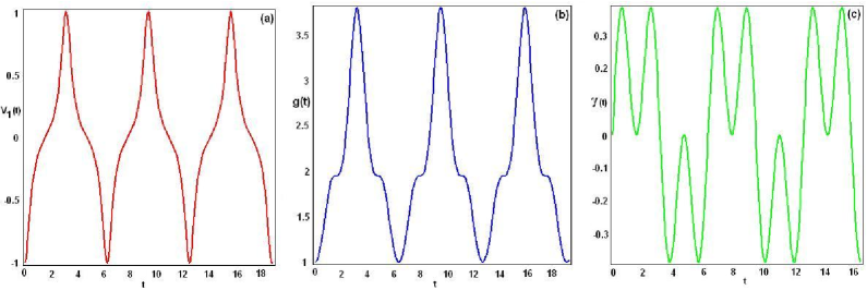
Figure 1: (color online). Profiles of the coefficients of the generalized ALH lattice with variable coefficients given by Eq. (5) vs time for the parameters given by Eq. (27) with parameters $\gamma_{0}=c_{1}=c_{2}=1$. (a) the coefficient $v_{1}(t)$ given by Eq. (20b) of the first degree term of the inhomogeneous frequency shift $v_{n}(t)$ given by Eq. (19b), (b) nonlinearity $g(t)$ given by Eq. (19a), and (c) the gain or loss term $\gamma(t)$.

IV Determining the similarity transformation and coefficients

It follows from Eqs. (17a)-(17) that we can obtain the variables $\rho(t),\,p_{1}(t)$ and $\tau(t)$ in transformation (15) in the form

$$\rho(t)=\rho_{0}\exp\left[-\int^{t}_{0}\gamma(s)ds\right],$$ (18a)

$$p_{1}(t)=\tan^{-1}\left[\frac{b\alpha(t)-a\beta(t)}{a\alpha(t)+b\beta(t)}\right],$$ (18b)

$$\tau(t)=(a^{2}\!+b^{2})^{-1/2}\int^{t}_{0}[\alpha^{2}(s)+\beta^{2}(s)]^{1/2}ds,$$ (18c)

where $\rho_{0}$ is an integration constant. Now it follows from Eqs. (17) and (17e) along with Eqs. (18a) and (18b) that we further find the inhomogeneous frequency shift $v_{n}(t)$ and intersite nonlinearity $g(t)$ in the form

$$g(t)=\rho_{0}^{-2}\exp\left[2\int^{t}_{0}\gamma(s)\,ds\right],$$ (19a)

$$v_{n}(t)=v_{1}(t)n+v_{0}(t),$$ (19b)

where we have introduced two functions in the inhomogeneous frequency shift $v_{n}(t)$ in the form

$$v_{1}(t)=\frac{\alpha(t)\dot{\beta}(t)-\dot{\alpha}(t)\beta(t)}{2[\alpha^{2}(t)+\beta^{2}(t)]},$$ (20b)

$$v_{0}(t)=a\left[\frac{\alpha^{2}(t)+\beta^{2}(t)}{a^{2}+b^{2}}\right]^{1/2}-\frac{\dot{p}_{0}(t)}{2},$$

where $p_{0}(t)$ is an arbitrary differentiable function of time.

It follows from Eqs. (19a)-(20b) that, in these coefficients of Eq. (5), the intersite nonlinearity $g(t)$ (the inhomogeneous frequency shift $v_{n}(t)$) is related to the gain or loss term $\gamma(t)$ (the tunnel coupling $\Lambda(t)=\alpha(t)+i\beta(t)$). This means that only two varying coefficients (e.g., $\gamma(t)$ and $\Lambda(t)=\alpha(t)+i\beta(t)$) are left free. Moreover, it follows from Eq. (19a) that the intersite nonlinearity $g(t)$ is always positive (i.e., the attractive intersite nonlinearity). In addition, it follows from Eq. (18a) that the gain or loss term $\gamma(t)$ can also control the function $\rho(t)$, which is used to modulate the amplitude of the complex field $\Psi_{n}(t)$.

For the inhomogeneous frequency shift $v_{n}(t)$ given by Eq. (19b), when $\alpha(t)\not=c\beta(t)$ with $c$ being a constant, the inhomogeneous frequency shift $v_{n}(t)$ is a linear function of space $n$ with coefficients being functions of time. In the absence of the discrete space $n$ in the inhomogeneous frequency shift, i.e., $v_{n}(t)\equiv v(t)$, which means that $\dot{p}_{1}(t)=0$ on the basis of Eq. (17), there exist two cases to be discussed:

i) If $p_{1}(t)\neq 0$ in which we have $p_{1}(t)=p_{1}={\rm const}\not=0$, then this means that $\varphi_{n}(t)$ is still a linear function of the discrete space $n$, i.e., $\varphi_{n}(t)=p_{1}n+p_{0}(t)$. In this case, the variable function $\tau(t)$ and the inhomogeneous frequency shift $v_{n}(t)$ are given by

$$\tau(t)=\frac{\int^{t}_{0}\alpha(s)ds}{a\cos(p_{1})+b\sin(p_{1})},\qquad\qquad\vspace{0.1in}$$

$$v_{n}(t)=\frac{a\alpha(t)}{a\cos(p_{1})+b\sin(p_{1})}-\frac{\dot{p}_{0}(t)}{2},\ \ \$$

and $\rho(t),\,g(t)$ are same as Eqs. (18a) and (19a);

ii) If $p_{1}(t)=0$, i.e., $\tan^{-1}\{[b\alpha(t)-a\beta(t)]/[a\alpha(t)+b\beta(t)]\}=0$, which means that the relation for the coefficients in Eq. (5), $\alpha(t)=(a/b)\beta(t)$, is required and $\varphi_{n}(t)$ is only a functions of time, i.e., $\varphi_{n}(t)\equiv p_{0}(t)$, then the variable function $\tau(t)$ and the inhomogeneous frequency shift $v_{n}(t)$ are given by the form

$$\tau(t)=\frac{1}{a}\int^{t}_{0}\alpha(s)ds,\quad v_{n}(t)=\alpha(t)-\frac{\dot{p}_{0}(t)}{2},$$

and $\rho(t),\,g(t)$ are same as Eqs. (18a) and (19a), where $\gamma(t),\ \alpha(t)$ and $p_{0}(t)$ are free functions of time, and $a,\ b,\ \rho_{0}$ are all free parameters.

V Nonautonomous discrete rogon solutions and interaction

In general, we have a large degree of freedom in choosing the coefficients of similarity transformation (15) and Eq. (5). As a consequence, we can obtain an infinitely large family of exact solutions of the generalized ALH lattice with variable coefficients given by Eq. (5) in terms of exact solutions of the discrete Hirota equation (10) and transformation (15). In particular, if we consider discrete rogon solutions of Eq. (10) as seeding solutions, then we can obtain many types of nonautonomous (including arbitrary time-dependent functions) discrete rogon (rogue wave) solutions of Eq. (5). As two representative examples, we consider the lowest-order discrete rogon solutions of Eq. (10) as two examples al to study the dynamics of nonautonomous discrete rogon solutions of Eq. (5).

V.1 Nonautonomous discrete one-rogon solution

Firstly, based on the similarity transformation (15) and one-rogon solution of the discrete Hirota equation (10), we present the nonautonomous discrete one-rogon solution (also known as the first-order rational solution) of Eq. (5) in the form

$$\Psi^{(1)}_{n}(t)\!=\!\rho_{0}\sqrt{\mu}\exp{\left\{-\int^{t}_{0}\gamma(s)ds+i[\varphi_{n}(t)+\hat{\varphi}_{n}(\tau)]\right\}}\hskip 28.45274pt$$

$$\times\left[1\!-\!\frac{4(1+\mu)\left[1+4i\mu\sqrt{a^{2}+b^{2}}\,\tau(t)\right]}{1+4\mu n^{2}+16\mu^{2}(1+\mu)(a^{2}+b^{2})\tau^{2}(t)}\right],$$ (22)

where the part phase $\hat{\varphi}_{n}(\tau)$ is defined by

$$\hat{\varphi}_{n}(\tau)\!=\!2\tau(t)\!\!\left[(1\!+\!\mu)\sqrt{a^{2}+b^{2}}\!-\!a\right]\!\!-\!n\tan^{\!-1}\!\left(b/a\right),\ \$$ (23)

$\mu$ is a positive parameter, the variable $\tau(t)$ is given by Eq. (18c), and the phase $\varphi_{n}(t)=p_{1}(t)n+p_{0}(t)$ with $p_{1}(t)$ given by Eq. (18b) and $p_{0}(t)$ being an arbitrary differentiable function of time.

To illustrate the wave propagations of the obtained nonautonomous discrete one-rogon solution (22), we can choose these free parameters in the form

$$\begin{array}[]{l}\alpha(t)=c_{1}\sin(2t),\quad\beta(t)=c_{2}\cos(t),\vspace{0.1in}\cr\gamma(t)=\gamma_{0}\sin(t)\cos^{2}(t),\vspace{0.1in}\cr a=b=\mu=\rho_{0}=1,\end{array}$$ (27)

where $\gamma_{0},\,c_{1,2}$ are constants.

Figure 1 depicts the profiles of the coefficient $v_{1}(t)=[\alpha(t)\dot{\beta}(t)-\dot{\alpha}(t)\beta(t)]/\{2[\alpha^{2}(t)+\beta^{2}(t)]\}$ of the first degree term of the inhomogeneous frequency shift $v_{n}(t)$ given by Eq. (20b), the attractive intersite nonlinearity $g(t)$ given by Eq. (19a), and the gain or loss term $\gamma(t)$ vs time for the parameters given by Eq. (27). The evolution of the intensity distribution for the one-rogon solution given by Eq. (22) is illustrated in Fig. 2 for parameters $\gamma_{0}=c_{1}=c_{2}=1$. The discrete rogue wave solution is localized both in space and in time, thus revealing the usual discrete ‘rogue wave’ features. However if we fix the coefficient $\gamma_{0}=1$ of the gain or loss term and adjust the coefficients $c_{1}=0.01,\ c_{2}=0.02$ of the tunnel couplings $\alpha(t)$ and $\beta(t)$ given by Eq. (27), then the evolution of the intensity distribution for the one-rogon solution is changed (see Fig. 3), and it follows from Fig. 3 that the discrete one-rogon solution in this case is localized in space and keep the localization longer in time than usual rogue waves (see al ). Moreover, it follows from Figs. 2(c) and 3(c) that the amplitude of the discrete one-rogon solution decreases as time increases, and the amplitude in Fig. 2(c) is decreased faster than one in Fig. 3(c) as time increases.

Figure 2: (color online). Profiles of nonautonomous discrete one-rogon solution (22) of the generalized ALH lattice with variable coefficients given by Eq. (5) for the parameters given by Eq. (27) with $\gamma_{0}=c_{1}=c_{2}=1$. (a) the intensity distribution $|\Psi_{n}^{(1)}(t)|^{2}$ with ${\rm max}_{(n,t)}|\Psi_{n}^{(1)}(t)|^{2}\cong 4.7$, (b) the density distribution $|\Psi_{n}^{(1)}(t)|^{2}$, (c) the intensity distributions $|\Psi_{n}^{(1)}(t)|^{2}$ for $t=0,\,0.2$, which means that the amplitude decreases as time increases, and the peak falls the lower position after time exceeds about $1$.

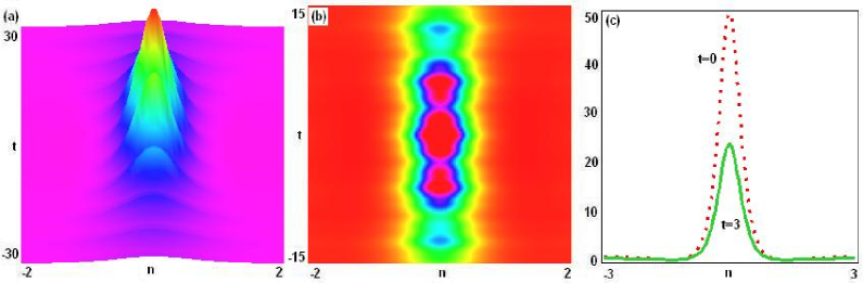
Figure 3: (color online). Profiles of nonautonomous discrete one-rogon solution (22) of the generalized ALH lattice with variable coefficients given by Eq. (5) for the parameters given by Eq. (27) with $\gamma_{0}=1,\,c_{1}=0.01$, and $c_{2}=0.02$. (a) the intensity distribution $|\Psi_{n}^{(1)}(t)|^{2}$ with ${\rm max}_{(n,t)}|\Psi_{n}^{(1)}(t)|^{2}\cong 43.2$, (b) the density distribution $|\Psi_{n}^{(1)}(t)|^{2}$, (c) the intensity distributions $|\Psi_{n}^{(1)}(t)|^{2}$ for $t=0,\,3$, which means that the amplitude decreases as time increases, and the peak falls the lower position after time exceeds about $70$.

V.2 The interaction between nonautonomous discrete rogon solutions

Here we consider the interaction between nonautonomous discrete rogon solutions. To do so, we apply a second-order rational solution of the discrete Hirota equation (10) to the similarity transformation (15) such that we can obtain the nonautonomous discrete two-rogon solution of Eq. (5) in the form

$$\Psi^{(2)}_{n}(t)=\rho_{0}\sqrt{\mu}\exp{\left\{\!-\!\int^{t}_{0}\!\gamma(s)ds+i[\varphi_{n}(t)+\hat{\varphi}_{n}(\tau)]\right\}}\quad$$

$$\times\!\!\left[1\!-\frac{\!12(1\!+\!\mu)\big{[}\mathcal{P}^{(2)}_{n}(\tau)\!+\!i\sqrt{\frac{\mathscr{T}(\tau)}{1+\mu}}\mathcal{Q}^{(2)}_{n}(\tau)\big{]}}{\mathcal{H}^{(2)}_{n}(\tau)}\right],\qquad$$ (28)

which displays the interaction between nonautonomous discrete rogon solutions, where $\mu$ is a positive parameter, the functions $\mathcal{P}^{(2)}_{n}(\tau),\,\mathcal{Q}^{(2)}_{n}(\tau)$ and $\mathcal{H}^{(2)}_{n}(\tau)$ are all polynomials of space and time given by

$$\begin{array}[]{l}\mathcal{P}^{(2)}_{n}(\tau)=5\mathscr{T}^{2}+6(\mathscr{N}+2\mu+3)\mathscr{T}+\mathscr{N}^{2}\vspace{0.1in}\cr\qquad\qquad\quad+(6-4\mu)\mathscr{N}-3(4\mu+1),\end{array}$$ (31)

$$\begin{array}[]{l}\mathcal{Q}^{(2)}_{n}(\tau)=\mathscr{T}^{2}+2(\mathscr{N}+1)\mathscr{T}+\mathscr{N}^{2}\vspace{0.1in}\cr\qquad\qquad\quad-(16\mu+6)\mathscr{N}-3(8\mu+5),\end{array}$$ (34)

$$\begin{array}[]{l}\mathcal{H}^{(2)}_{n}(\tau)\!=\!\mathscr{T}^{3}\!+\!3(\mathscr{N}\!+\!8\mu+9)\mathscr{T}^{2}\!+\!3(\mathscr{N}^{2}\!-\!6\mathscr{N}\vspace{0.1in}\cr\qquad\qquad\quad\!-\!16\mu\mathscr{N}\!+\!48\mu^{2}\!+\!72\mu\!+\!33)\mathscr{T}\!+\!\mathscr{N}^{3}\vspace{0.1in}\cr\qquad\qquad\quad\!+\!(3-8\mu)\mathscr{N}^{2}\!+\!(27+24\mu+16\mu^{2})\mathscr{N}\!+\!9,\end{array}$$ (38)

where we have introduced $\mathscr{N}=4\mu n^{2}$ and $\mathscr{T}=16\mu^{2}(1+\mu)(a^{2}+b^{2})\tau^{2},$ $\tau\equiv\tau(t)$ is given by Eq. (18c), the part phase $\varphi_{n}(t)=p_{1}(t)n+p_{0}(t)$ with $p_{1}(t)$ given by Eq. (18b) and $p_{0}(t)$ being an arbitrary differentiable function of time, and the part phase $\hat{\varphi}_{n}(\tau)$ is given by Eq. (23).

Similarly, we can choose these free parameters given by Eq. (27) for the nonautonomous discrete two-rogon solution given by Eq. (28) except for $\mu=1/16$. Figures 4 and 5 depict the evolution of intensity distribution for the interaction between nonautonomous discrete rogon solutions (discrete two-rogon solution) given by Eq. (28) for different parameters $\gamma_{0},\,c_{1}$, and $c_{2}$, respectively. Moreover, we find that the interaction between nonautonomous discrete rogue waves is elastic. Figure 4 shows that the nonautonomous discrete two-rogon solution is localized both in space and in time, thus revealing the usual discrete ‘rogue wave’ features for the chosen parameters $\gamma_{0}=1,\,c_{1}=2,\,c_{2}=1$, but if we fix the coefficient $\gamma_{0}=1$ of the gain or loss term and adjust the coefficients $c_{1}=0.2,\ c_{2}=0.1$ of the tunnel couplings $\alpha(t)$ and $\beta(t)$ given by Eq. (27), then the evolution of the intensity distribution for the discrete two-rogon solution is changed (see Fig. 5), and it follows from Fig. 5 that the nonautonomous discrete two-rogon solution is localized in space and keep the localization longer in time than usual rogue waves. Moreover, it follows from Figs. 4(c) and 5(c) that the amplitude of the discrete two-rogon solution decreases as time increases, and the amplitude in Fig. 4(c) decreases faster than one in Fig. 5(c) as time increases.

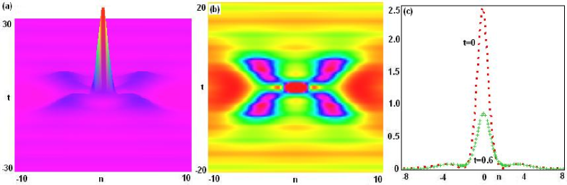
Figure 4: (color online). Profiles of the interaction between nonautonomous discrete rogon solution given by Eq. (28) of the generalized ALH lattice with variable coefficients given by Eq. (5) for the parameters given by Eq. (27) with $\gamma_{0}=1,\,c_{1}=2$, and $c_{2}=1$. (a) the intensity distribution $|\Psi_{n}^{(2)}(t)|^{2}$ with ${\rm max}_{(n,t)}|\Psi_{n}^{(2)}(t)|^{2}\cong 1.65$, (b) the density distribution $|\Psi_{n}^{(2)}(t)|^{2}$, (c) the intensity distributions $|\Psi_{n}^{(2)}(t)|^{2}$ for $t=0,\,0.6$, which means that the amplitude decreases as time increases, and the peak falls the lower position after time exceeds about $3$.

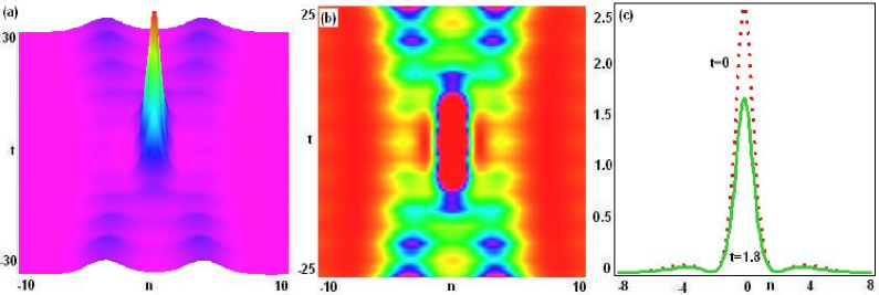
Figure 5: (color online). Profiles of the interaction between nonautonomous discrete rogon solution given by Eq. (28) of the generalized ALH lattice with variable coefficients given by Eq. (5) for the parameters given by Eq. (27) with $\gamma_{0}=1,\,c_{1}=0.2$, and $c_{2}=0.1$. (a) the intensity distribution $|\Psi_{n}^{(2)}(t)|^{2}$ with ${\rm max}_{(n,t)}|\Psi_{n}^{(2)}(t)|^{2}\cong 2.25$, (b) the density distribution $|\Psi_{n}^{(2)}(t)|^{2}$, (c) the intensity distributions $|\Psi_{n}^{(2)}(t)|^{2}$ for $t=0,\,1.8$, which means that the amplitude decreases as time increases, and the peak falls the lower position after time exceeds about $65$.

VI Conclusions

In conclusion, we have studied nonautonomous discrete rogon solutions and their interaction in the generalized Ablowitz-Ladik-Hirota lattice with the varying tunnel coupling, intersite nonlinearity, inhomogeneous frequency shift, and gain or loss term given by Eq. (5) on the basis of the differential-difference similarity reduction (15). We found its some nonautonomous discrete rogon solutions when the intersite nonlinearity $g(t)$ (the inhomogeneous frequency shift $v_{n}(t)$) is related to the gain or loss term $\gamma(t)$ (the tunnel coupling $\Lambda(t)=\alpha(t)+i\beta(t)$) (see Eqs. (19a) and (19b)). This denotes that only two coefficients (i.e., $\gamma(t)$ and $\Lambda(t)=\alpha(t)+i\beta(t)$) are left free.

In particular, we have studied wave propagations of nonautonomous discrete rogon solutions and interaction for some chosen parameters, which exhibit complicated rogue wave construes. For the given periodic gain or loss term, when the amplitude of the tunnel coupling coefficient between sites decreases, these nonautonomous discrete rogon solutions are localized in space and keep the localization longer in time, which differ from the usual discrete rogue waves of nonlinear discrete equations (e.g., the AL lattice and the discrete Hirota equation) al .

Moreover, nonautonomous discrete rogon solutions and interaction may provide more documents to further understand the physical mechanism of discrete rogue wave phenomena. The approach may also be extended to other discrete nonlinear lattices with variable coefficients for studying their discrete rogue wave solutions and wave propagations.

- (1) N. Akhmediev, A. Ankiewicz, and M. Taki, Phys. Lett. A 373, 675 (2009); N. Akhmediev, A. Ankiewicz, and J. M. Soto-Crespo, Phys. Rev. E 80, 026601 (2009); A. Ankiewicz, J. M. Soto-Crespo, and N. Akhmediev, Phys. Rev. E 81, 046602 (2010); A. Ankiewicz, P. A. Clarkson, and N. Akhmediev, J. Phys. A 43, 122002 (2010).
- (2) Z. Y. Yan, Phys. Lett. A 374, 672 (2010).
- (3) C. Kharif and E. Pelinovsky, Euro. J. Mech. B/Fluids 22, 603 (2003).
- (4) K. Dysthe, H. E. Krogstad, and P. Müller, Annu. Rev. Fluid Mech. 40, 287 (2008).
- (5) D. R. Solli, C. Ropers, P. Koonath, and B. Jalali, Nature (London) 450, 1054 (2007).
- (6) D. R. Solli, C. Ropers, and B. Jalali, Phys. Rev. Lett. 101, 233902 (2008).
- (7) B. Kibler, J. Fatome, C. Finot, G. Millot, F. Dias, G. Genty, N. Akhmediev, and J. M. Dudley, Nature Phys. 6, 1 (2010).
- (8) Y. V. Bludov, V. V. Konotop, and N. Akhmediev, Phys. Rev. A 80, 033610 (2009).
- (9) L. Stenflo and M. Marklund, J. Plasma Phys. 76, 293 (2010).
- (10) Z. Y. Yan, Commun. Theor. Phys. 54, 947 (2010) [e-print, arXiv:0911.4259].
- (11) Y. C. Ma, Stud. Appl. Math. 60, 43 (1979).
- (12) D. H. Peregrine, J. Aust. Math. Soc. Ser. B, Appl. Math. 25, 16 (1983).
- (13) A. Ankiewicz, N. Devine, and N. Akhmediev, Phys. Lett. A 373, 3997 (2009).
- (14) Z. Y. Yan, V. V. Konotop, and N. Akhmediev, Phys. Rev. E 82, 036610 (2010); Z. Y. Yan, J. Math. Anal. Appl. 380, 689 (2011).
- (15) J. C. Eilbeck, P. S. Lomdahl, and A. C. Scott, Physica D 16, 318 (1985).
- (16) M. J. Ablowitz and J. F. Ladik, Stud. Appl. Math. 55, 213 (1976).
- (17) M. J. Ablowitz and J. F. Ladik, J. Math. Phys. 17, 1011 (1976).
- (18) D. Hennig and G. P. Tsironis, Phys. Rep. 307, 333 (1999).
- (19) Y. V. Kartashov, B. A. Malomed, and L. Torner, Rev. Mod. Phys. 83, 247 (2011).
- (20) M. J. Ablowitz, B. Prinari, and A. D. Trubatch, Discrete and continuous nonlinear Schrödinger systems (Cambridge University Press, Cambridge, 2004).
- (21) P. G. Kevrekidis, The Discrete Nonlinear Schrödinger Equation: Mathematical Analysis, Numerical Computations and Physical Perspectives (Springer, Berlin, 2009).
- (22) F. Lederer, G. I. Stegeman, D. N. Christodoulides, G. Assanto, M. Segev, and Y. Silberberg, Phys. Rep. 463, 1 (2008).
- (23) S. Takeno and K. Hori, J. Phys. Soc. Jpn. 59, 3037 (1990).
- (24) Y. S. Kivshar and D. K. Campbell, Phys. Rev. E 48, 3077 (1993).
- (25) M. Salerno, Phys. Rev. A 46, 6856 (1992).
- (26) D. Cai, A. R. Bishop, N. Grnbech-Jensen, and B. A. Malomed, Phys. Rev. E 50, R694 (1994); D. Cai, A. R. Bishop, and N. Gronbech-Jensen, Phys. Rev. Lett. 72, 591 (1994).
- (27) Y. Kivshar and M. Salerno, Phys. Rev. E 49, 3543 (1994).
- (28) V. V. Konotop and M. Salerno, Phys. Rev. E 55, 4706 (1996).
- (29) Z. W. Xie, Z. X. Cao, E. I. Kats, and W. M. Liu, Phys. Rev. A 71, 025601 (2005).
- (30) A. Trombettoni and A. Smerzi, Phys. Rev. Lett. 86, 2353 (2001); J. Gomez-Gardenẽs, B. A. Malomed, L. M. Floría, and A. R. Bishop, Phys. Rev. E 73, 036608 (2006); ibid, 74, 036607 (2006).
- (31) Y. V. Bludov, V. V. Konotop, and N. Akhmediev, Opt. Lett. 34, 3015 (2009).
- (32) A. Maluckov, Lj. Hadz̆ievski, N. Lazarides, and G. P. Tsironis, Phys. Rev. E 79, 025601R (2009).
- (33) A. Ankiewicz, N. Akhmediev, and J. M. Soto-Crespo, Phys. Rev. E 82, 026602 (2010).
- (34) N. Akhmediev and A. Ankiewicz, Phys. Rev. E 83, 046603 (2011).
- (35) K. Narita, J. Phys. Soc. Jpn. 59, 3528 (1990); ibid, 60, 1497 (1991).
- (36) B. Mieck and R. Graham, J. Phys. A 38, L139 (2005).
- (37) M. J. Ablowitz and J. F. Ladik, Stud. Appl. Math. 57, 1 (1977).
- (38) M. Daniel and K. Manivannan, J. Math. Phys. 40, 2560 (1999).
- (39) R. Hirota, J. Math. Phys. 14, 805 (1973).
- (40) Y. S. Kivshar and G. P. Agrawal, Optical solitons: from fibers to photonic crystals (Academic Press, New York, 2003); B. A. Malomed, D. Mihalache, F. Wise, and L. Torner, J. Opt. B: Quantum Semiclassical Opt. 7, 53R (2005).
- (41) G. P. Agrawal, Nonlinear Fiber Optics (4th. Ed., Academic Press, San Diego, 2007); A. Hasegawa and Y. Kodama, Solitons in Optical Communications (Clarendon Press, Oxford, 1995).
- (42) S. A. Ponomarenko and G. P. Agrawal, Phys. Rev. Lett. 97, 013901 (2006); V. N. Serkin, A. Hasegawa, and T. L. Belyaeva, ibid. 98, 074102 (2007); J. Belmonte-Beitia, V. M. P erez-Garcia, V. Vekslerchik, and P. J. Torres, ibid. 98, 064102 (2007); Z. Y. Yan, Phys. Lett. A 361, 223 (2007); Z. Y. Yan, Phys. Scr. 75, 320 (2007). Z. Y. Yan and V. V. Konotop, Phys. Rev. E 80, 036607 (2009); Z. Y. Yan and C. Hang, Phys. Rev. A 80, 063626 (2009).