Diagnostics of electron beam properties from the simultaneous hard X-ray and microwave emission in the 10 March 2001 flare

Abstract

Context. Microwave (MW) and hard X-ray (HXR) data are thought to be powerful means for investigating the mechanisms of particle acceleration and precipitation in solar flares reflecting different aspects of electrons interaction the ambient particles in a presence of magnetic field. Simultaneous simulation of HXR and MW emission with the same populations of electrons is still a great challenge for interpretation of observations in real events. Recent progress in simulations of particle kinetics with time-dependent Fokker–Planck (FP) approach offers an opportunity to produce such the interpretation.

Aims. In this paper we apply the FP kinetic model of precipitation of electron beam with energy range from 12 keV to 1.2 MeV to the interpretation of X-ray and microwave emissions observed in the flare of 10 March 2001.

Methods. The theoretical HXR and MW emissions were calculated by using the distribution functions of electron beams found by solving time-dependent Fokker–Planck approach in a converging magnetic field (Zharkova at al., 2010; Kuznetsov and Zharkova, 2010) for anisotropic scattering of beam electrons on the ambient particles in Coloumb collisions and Ohmic losses.

Results. The simultaneous observed HXR photon spectra and frequency distribution of MW emission and polarization were fit by those simulated from FP models which include the effects of electric field induced by beam electrons and precipitation into a converging magnetic loop. Magnetic field strengths in the footpoints on the photosphere were updated with newly calibrated SOHO/MDI data. The observed HXR energy spectrum above 10 keV is shown to be a double power law which was fit precisely by the photon HXR spectrum simulated for the model including the self-induced electric field but without magnetic convergence. The MW emission simulated for different models of electron precipitation revealed a better fit(above $90\%$ confidence level) to the observed distribution at higher frequencies for the models combining collisions and electric field effects with a moderate magnetic field convergence of 2. The MW simulations were able to reproduce closely the main features of the MW emission observed at higher frequencies: the spectral index, the frequency of peak intensity and the frequency of the MW polarisation reversal while at lower frequencies the simulated MW intensities are lower than the observed ones.

1 Introduction

Spatial configurations of flaring sites in hard X-ray (HXR) and microwave (MW) emissions are highly variable, they may be formed by a single loop with one coronal source and two footpoints (Masuda et al. 1994; Kundu et al. 2001b) or several sets of loops with a few footpoints and coronal sources (Hanaoka 1996; Kundu et al. 2001a) leading to different models for different types of flaring events (see the review by Melrose (1999)).

Simultaneous observations of hard X-ray emission and microwaves in footpoints of solar flares often show their close temporal correlation pointing out to their common origin (Aschwanden 2005; Bastian et al. 1998). There is a high likelihood that these emissions are produced by the same population of non-thermal electrons (Kundu 1985; Kundu et al. 2001a, b, 2004; Vilmer et al. 2002; Wilson & Holman 2003; Kundu et al. 2009).

However, there are substantial discrepancies in the locations of these HXR and MW sources observed in the same flare — e.g., they are often separated from each other, and the areas covered by each emission are substantially different. Observations often suggest that the sources of MW and HXR emission may be separated in depths within a flaring loop (Kundu 1985; Takakura et al. 1995; Sui et al. 2002). The intensities of HXR and MW emissions in the opposite legs of the same flaring loop can be strongly anti-correlated being in one footpoint of the same loop higher in MW and lower in HXR emission, while in the other footpoint being higher in HXR and lower in MW emission (Kundu 1985; Takakura et al. 1995; Kundu et al. 2004; Grechnev et al. 2008). In addition, there is sometimes a delay between HXR and MW emissions occurring in the same flare (Kundu et al. 1995, 2004; Sui et al. 2002).

MW emission demonstrates a high variability of polarization from a few percent (Altyntsev et al. 2000; Fleishman & Melnikov 2003; Fleishman et al. 2003) up to 50–100% (Dulk 1985; Altyntsev et al. 2000; Lee & Gary 2000). Unlike HXR emission, which properties are controlled by the parameters of emitting electrons and ambient plasma particles and Compton backscattering, i.e. albedo effects (Kontar et al. 2006) , MW emission is determined in addition by various radiative transfer effects. Nevertheless, general perception of MW polarization is that highly collimated electron beams tend to produce MW emission with a higher polarization degree (Fleishman & Melnikov 2003; Fleishman et al. 2003; Melnikov et al. 2008; Fleishman & Kuznetsov 2010).

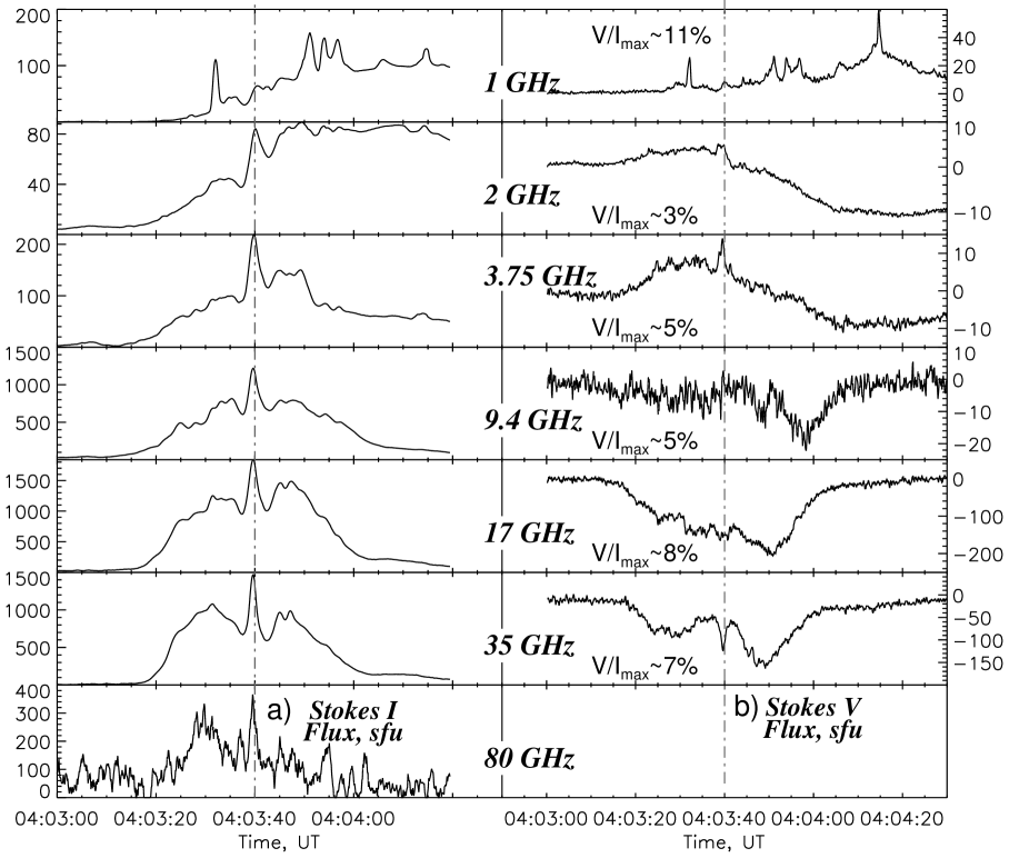
Figure 1: The 10 March 2001 event. Time profiles of the average brightness temperature at 1–80 GHz (NoRP) in total intensity (a) and polarization (b). (V/I)_max is the maximum degree of polarization at the central peak (04:03:40). The numbers in Y axes are in the solar flux units (sfu).

Moreover, the resulting photon spectra of HXR and MW emission produced during flares are also significantly different. In particular, HXR emission from strongest flares often has the elbow-type spectra with double power-law energy distributions (Lin et al. 2003; Holman et al. 2003) and noticeable differences between the spectral indices at lower (below 70 keV) and higher energies. MW distribution in frequency (Dulk 1985; Bastian et al. 1998) has a maximum with a gradual decrease of the intensity towards lower frequencies (optically thick emission) and a negative power law distribution towards higher frequencies (optically thin emission). The peak frequency usually varies from 3 to 20 GHz for different flares or different stages of the same flare (Nita et al. 2004; Melnikov et al. 2008).

These differences clearly indicate different transport scenarios for high-energy particles precipitating into the footpoints of a flaring loop. The mechanisms of transport affecting HXR and MW emissions are well known to be substantially different: MW radiation is related to gyrosynchrotron emission of high-energy electrons with energies from few tens keV (Kundu et al. 2001a) up to several MeV (Bastian 1999; Kundu et al. 2004), while HXR radiation is often produced by the electrons with much lower energies from 10 to 300 keV (see, for example, Lin et al. 2003; Holman et al. 2003). In spite of a large number of simulations for the interpretation of HXR and MW emission with thick target models (see, for example, reviews Fleishman & Melnikov 2003; Fleishman et al. 2003; Fleishman & Kuznetsov 2010; Krucker et al. 2008, 2010, and references therein), so far there are only a few simulations (Melnikov et al. 2008; Kuznetsov & Zharkova 2010) considering the problem of particle transport in other than collisional energy loss mechanisms and their effects on HXR and MW emission.

However, recent kinetic models calculated electron distribution functions numerically by solving the time-dependent Fokker–Planck kinetic equation for precipitation of electron beams into a flaring atmosphere with converging magnetic field. Beam electrons with an energy range from 12 keV to 10 MeV are assumed to lose their energy and change propagation directions in collisions and due to Ohmic losses in the electric field induced by the beam (Diakonov & Somov 1988; Zharkova et al. 1995; Zharkova & Gordovskyy 2006; Battaglia & Benz 2008) and due to scattering in converging magnetic field (Leach & Petrosian 1981; McClements 1992a, b; Siversky & Zharkova 2009). These solutions were applied for the explanation of HXR emission produced by solar flares which provided a very good fit for HXR intensities (McClements 1992b), directivity and polarization (Zharkova et al. 2010). Recent extension of these solutions to the interpretations of MW emission from solar flares appears to produce promising results in closer fitting to observations (Kuznetsov & Zharkova 2010).

These kinetic models can be further tested by the simultaneous interpretation of HXR and MW emission observed in the same flare. For this purpose we selected the flare of the 10 March 2001 that has been extensively studied (Liu et al. 2001; Ding 2003; Uddin et al. 2004; Chandra et al. 2006; Altyntsev et al. 2008; Melnikov et al. 2008) because of the following reasons: 1) it had produced both kinds, HXR and MW emissions, MW with a pronounced polarization; 2) it was a rather powerful flare which had to be produced by powerful electron beams allowing one to explore the effects of various energy loss mechanisms on HXR and MW emissions; and 3) it was located far from the disk centre that allows us to compare the energy loss effects in a flaring atmosphere seen by an observer from the Earth at larger viewing angles.

The first detailed analysis of a spatial dynamics of this flare in HXR and MW emissions was made by Chandra et al. (2006). They showed that the spatial structure derived from the microwave emission allows one to assume an interaction between two loops, one of which was a small, newly emerging loop, while the other was a large overlying loop, similar to the events identified by Hanaoka (Hanaoka 1996, 1999a, 1999b).

Later Altyntsev et al. (2008) also interpreted the high-frequency MW emission in this event produced by electrons precipitating into a homogeneous source or into two homogeneous sources located in two loop legs where the depth variations of the parameters of high energy electrons, plasma density and magnetic field were neglected. The authors though concluded that such electrons were rather anisotropic, or beamed, because (i) the microwave emission consisted of many short (the order of seconds) broadband pulses supposedly marking quite a few elementary acts of beam injection into the loop legs, (ii) the microwave emission was O-mode polarized at 17 GHz (optically thin part of the spectrum) meaning that the observed MW emission was an immediate outcome of the beam precipitation rather than the radiative transfer effects, (iii) type III-like drifting bursts were observed at lower frequencies meaning that beam electrons streamed to higher atmospheric levels.

The goal of the current research is to extend the investigation of this flare to simultaneous interpretation of HXR and MW emissions and to fit their observed energy distributions with the simulations of electron precipitation into a converging magnetic loop by using the Fokker–Planck kinetic approach taking into account collisional and Ohmic losses in the electric field induced by well collimated beam electrons. Observations are described in section 2, the model and method of simulations are described in section 3, the results of the model fit to observations are shown in section 4 and the conclusions are drawn in section 5.

2 Observations

2.1 Instrumentation

We used microwave total flux records from Nobeyama Radio Polarimeters (NoRP; Torii et al. 1979; Shibasaki et al. 1979; Nakajima et al. 1985) at 1, 2, 3.75, 9.4, 17, 35, and 80 GHz. The time resolution of routine NoRP data available at the NoRP Web site is 1 s, and for flares it is 0.1 s. Nobeyama Radioheliograph (Nakajima et al. 1994) produces images at 17 and 34 GHz. The imaging interval of the flare mode data which we used in this work was 0.1 s.

The line-of-sight magnetograms have been produced with the Michelson Doppler Imager (MDI; Scherrer et al. 1995) on SOHO. The full disk magnetograms with a resolution of 1.98^′′ re-calibrated in December, 2008 were obtained from the Solar Data Information Centre at Stanford University, US.

Information about HXR emission was supplied by instruments on Yohkoh satellite (Kosugi et al. 1991a, b). Images of HXR sources and fluxes with a high temporal resolution (0.5 s) were obtained from Hard X-Ray Telescope (HXT) data. HXT carried out observations in four spectral bands: L, 14–23 keV; M1, 23–33 keV; M2, 33–53 keV; H, 53–93 keV. The spectra were obtained from data of the Hard X-ray Spectrometer (HXS), which was one sensor of the Wide Band Spectrometer (WBS; Yoshimori et al. 1991; Sato et al. 2006). HXS data provided hard X-ray spectra in a wide energy range of 20–657 keV. The temporal resolution of HXS data was 4 s, i.e., slightly lower than the temporal resolution of HXT.

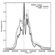
Figure 2: Light curves of the HXR burst registered in the HXT/M2 channel (33–53 keV) and the HXS record integrated over the whole band (20–657 keV, histogram) along with the microwave burst registered by NoRP at 17 GHz. The vertical dotted line marks the main peak under consideration at 04:03:40 UT.

2.2 HXR and MW bursts and their sources

The 1B/M6.7 flare of 10 March 2001 associated with a CME occurred in active region 9368 (N27W42) and was previously studied in detail in a number of papers listed above. However, recent re-calibration of magnetic field strengths in SOHO/MDI magnetograms alerted a review of previous results and inspired an analysis of additional observations, which were not yet considered.

2.2.1 Light curves of MW and HXR emissions

As found by Altyntsev et al. (2008), broadband short pulses were present in the whole frequency range 1–80 GHz of NoRP (see time profiles in Fig. 1a). The MW time profiles in total intensity at different frequencies were very similar. Three main peaks are detectable in the MW burst with a total duration of about 40 s (see Fig. 1a). The first MW peak at about 04:03:30.90 (all times hereafter are UT) was the lowest one, the second (central) MW peak at 04:03:40 with a total duration of about 5 s was the highest one. The third MW peak had a double structure with two sub-peaks occurring at 04:03:44.90 UT and 04:03:46.80 UT, respectively.

The time profiles of the polarized MW emission (Stokes V component) around the central peak are shown in Fig. 1b. They coincide with the light curves shown by Altyntsev et al. (2008). The MW emissions of all the three peaks had a positive (right-handed) circular polarization (RCP) at low frequencies (1–3.75 GHz), and their polarization at higher frequencies (9.4–35 GHz) was negative (left-handed, LCP), as Fig. 1b shows.

In order to understand the dynamics of high-energy particles in this flare, let us also use the whole energy range of the HXR emission recorded by Yohkoh/HXS and estimate parameters of the electron beam, thus extending studies carried out by Altyntsev et al. (2008) and Chandra et al. (2006) that were confined to the MW emission.

This flare was observed by Yohkoh/HXT in four energy channels L, M1, M2, and H. Thus, the available energy bands of HXR channels allowed us to derive photon spectra up to 600 keV. The HXS light curve presenting the integrated flux within 20–657 keV range is plotted along with HXT and NoRP data as shown in Fig. 2. The HXS light curve is plotted as a histogram to reveal its temporal correspondence with the HXR and NoRP data. Sometimes the HXS time bin could contain the emission integrated over two peaks seen by HXT and at 17 GHz (for example, this happened at about 04:03:47). Fortunately, the temporal variations of HXR and NoRP emissions during the main peak resemble the HXS light curve.

The time profiles of the HXR and 17 GHz emissions have a close temporal correlation (Fig. 2). Nevertheless, there are some delays of HXR emission relative to microwaves. They amount to a fraction of second at high frequencies and reach 1–2 s at low frequencies (Altyntsev et al. 2008).

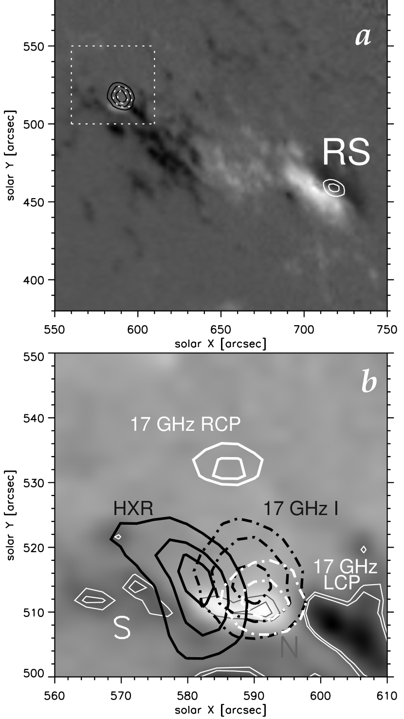
Figure 3: a) Contours of 17 GHz (NoRH, 04:04) flare sources (black solid: Stokes I, 50%, 70% ,90% of the maximum, white solid: Stokes V, RCP, 70%, 90% of the maximum, white dotted: Stokes V, LCP, 70%, 90% of the minimum) superimposed on an MDI magnetogram (04:48:01.61, light areas represent N-polarity, dark areas show S-polarity). The axes show hereafter arc seconds from the solar disk centre. b) Enlarged flare site denoted in panel (a) by the broken frame. Contours of 17 GHz (NoRH, 04:03:40) Contours levels are the same. Black thick contours correspond to the HXR source (Yohkoh/HXT/H; 04:03:40.25; 20%, 50%, 80% of the maximum). Thin solid gray contours mark N-polarity [levels 600, 800 G], and thin white contours mark S-polarity [levels $-600$, $-500$ G].

2.2.2 MW and HXR images

The flare was triggered by an interaction between two loops, one of which was a small, newly emerging loop, while the other was a large overlying loop (Chandra et al. 2006). The two loops formed a ‘three-legged’ configuration in which the magnetic field had a ‘bipolar + remote unipolar’ structure. The footpoints of the small loop (main flare source) can be seen in HXR/H and MW images (Fig. 3b) whose position is denoted by the white dotted frame in Fig. 3a. The magnetogram taken at 04:48:30 was compensated for the differential rotation to 04:03:40 (the most prominent peak time). The magnetic field strengths were projection-corrected using the zradialize SolarSoftware routine (Fig. 3). The length of the loop visible in an EIT 195 Å image is 10000 km according to Altyntsev et al. (2008). During the flare, the NoRH beam size was about $20.6^{\prime\prime}\times 17.3^{\prime\prime}$ at 17 GHz and $9.5^{\prime\prime}\times 3.9^{\prime\prime}$ at 35 GHz.

The bulk of the MW emission at 17 GHz during the main peak was generated from the small loop. At the onset of the burst an LCP source located in the N-polarity magnetic field (Fig. 3b) was observed. An RCP source appeared north of the LCP source at 04:03:27 in the S-polarity magnetic field, meaning that they both were polarized in the sense of the O-mode.

The magnitude of the field in the spot labelled “N” (solid thin gray contours in Fig. 3b) reached 800 G and for the S-polarity field labelled “S” it reached 600 G. The large loop had footpoints in the main and remote (RS) sources (Fig. 3a). RS appeared at 04:03:51 and had a right circular polarization at 17 GHz. The right polarization in the main source disappeared after 04:03:52.

At the onset of the flare (04:03:12) a single compact source was only seen in all energy channels of Yohkoh/HXT. HXR images obtained with a 4-s cadence in the L channel showed that the source expanded and got elongated by 04:04:05. In the H channel, the compact source transformed to a loop-like one by 04:03:25, and by 04:04:05 it became compact again. The distance between the centroids of the radio and HXR sources was about 10^′′.

For calculations of HXR spectra one needs areas of emitting sources. We estimated the sizes of the sources obtained in all four Yohkoh/HXT energy channels by fitting them with ellipses at half magnitude for the positions as if these sources would be located at the solar disk centre to exclude projection effects. The estimated sizes of the HXR sources are $16^{\prime\prime}\times 12.6^{\prime\prime}$, $18^{\prime\prime}\times 12.2^{\prime\prime}$, $15.4^{\prime\prime}\times 12^{\prime\prime}$, and $12^{\prime\prime}\times 16.8^{\prime\prime}$ for the L, M1, M2, and H channel, respectively.

3 Model simulations

3.1 Description of the model

Let us consider the time-dependent Fokker–Planck approach for precipitation of high-energy electrons injected into a cold hydrogen plasma confined in a converging magnetic field structure (Leach & Petrosian 1981; Siversky & Zharkova 2009) while producing a self-induced electric field, which forms a return current from the ambient plasma and beam electrons (Knight & Sturrock 1977a; Emslie 1980). We take account of collisions, Ohmic losses and pitch-angle anisotropy in scattering on ambient particles (Diakonov & Somov 1988; McClements 1992a; Zharkova et al. 2010).

There are the two basic expression to describe the problem: a kinetic Fokker–Planck–Landau equation for beam electrons, and the Ampere law for the neutralization of electric currents formed from the direct and returning beams. A distribution function $f$ of beam electrons is governed by Fokker–Planck, or Landau, equation (Landau 1937):

$$\frac{\partial f}{\partial t}+V\cos\alpha\frac{\partial f}{\partial z}-e\mathcal{E}V\cos\alpha\frac{\partial f}{\partial E}-\frac{e\mathcal{E}\sin^{2}\alpha}{m_{\mathrm{e}}V}\frac{\partial f}{\partial\cos\alpha}$$

$$=\left(\frac{\partial f}{\partial t}\right)_{\mathrm{coll}}+\left(\frac{\partial f}{\partial t}\right)_{\mathrm{magn}},$$ (1)

where $z$ is a linear depth measured from the top of a coronal loop, $E$ and $\alpha$ are the electron energy and pitch angle, respectively, $V$ is the electron speed, and $e$ and $m_{\mathrm{e}}$ are the electron charge and mass, respectively. The first term on the left-hand side describes variations of the distribution function in time ($t$), the second term describes its variations with depth ($z$), the third and the fourth terms reflect energy losses owing to Ohmic heating and pitch-angular diffusion under the presence of a self-induced electric field $\mathcal{E}$. The two terms on the right-hand side $(\partial f/\partial t)_{\mathrm{coll}}$ and $(\partial f/\partial t)_{\mathrm{magn}}$ describe the energy of a particle and the pitch-angle diffusion caused by scattering on ambient particles (collisional integral) and in a converging magnetic field, respectively.

The collisional integral is taken in the linearized form suggested by Diakonov & Somov (1988), considering variations of collisional energy losses and anisotropic scattering with pitch angle diffusion for a given kinetic temperature of the ambient plasma and distribution function $f$ of beam electrons as follows

$$\left(\frac{\partial f}{\partial t}\right)_{\mathrm{coll}}=\frac{1}{v^{2}}\frac{\partial}{\partial v}\left[v^{2}\nu(E)\left(\frac{k_{\mathrm{B}}T_{\mathrm{e}}}{m_{\mathrm{e}}}\frac{\partial f}{\partial v}+vf\right)\right]$$

$$+\nu(E)\frac{\partial}{\partial\cos\alpha}\left(\sin^{2}\alpha\frac{\partial f}{\partial\cos\alpha}\right).$$ (2)

Here $k_{\mathrm{B}}$ is the Boltzmann gas constant, $T_{\mathrm{e}}(\xi)$ is the ambient electron temperature at column depth $\xi$ and $\nu(E)$ is the frequency of collisions taken as follows

$$\nu(E)=\frac{4k}{3}\frac{\sqrt{2\pi}}{m_{\mathrm{e}}}ne^{4}\lambda(\xi)\,E^{-3/2},$$

where $n$ is the ambient plasma density, $E$ is the beam electron energy, $\lambda(\xi)$ is the Coulomb logarithm for collisions of beam electrons with the ambient ones for a column depth $\xi$, and the parameter $k$ is taken in the form (Emslie 1978)

$$k=2x\,+\,(1-x)\frac{\lambda^{\prime\prime}-\lambda^{\prime}}{\lambda},$$

where $\lambda^{\prime\prime}$ and $\lambda^{\prime}$ are the Coloumb logarithms for collisions of beam electrons with the ambient ions and neutrals, respectively.

The linear coordinate $z$ is replaced by the column density$\xi(z)=\int\limits_{z_{\min}}^{z}n(s)\,\mathrm{d}s$(Diakonov & Somov 1988; Siversky & Zharkova 2009). The effect of the magnetic field convergence variations with column density is described by the semi-empirical expression Siversky & Zharkova (2009) with the characteristic column depth of $10^{20}$ $cm^{-2}$, allowing to match the observations of magnetic field magnitudes at the photosphere and chromosphere (Kontar et al. 2008). This semi-empirical form was further modified by Siversky & Zharkova (2009) for the magnetic field distribution with a linear depth, required for the simulation of MW emission.

3.1.1 Self-induced electric field

The problem of electrostatic electric field carried by beam electrons and the return current formed by the ambient plasma was discussed in the past decades by many authors (see, for example Knight & Sturrock 1977b; Emslie 1980, and the references therein). Brown & Bingham (1984) concluded that a return current can be established electro-statically because of large radii of electron beams inside flaring atmospheres that implies very long resistive timescales along the finite beam lengths leading to negligible inductive effects compared to the electrostatic ones even for plasma with anomalous resistivity. The full electro-magnetic approach carried out by van den Oord (1990) to study of electric and magnetic fields induced by precipitating electron beams and their interaction with electrostatic field carried by these electrons allowed to conclude that the both electric fields: electrostatic and induced ones co-exist in a flaring atmosphere and are neutralised by the electrostatic or solenoidal response of the ambient plasma.

These two plasma responses are found to act independently (Brown & Bingham 1984; van den Oord 1990) forming from one side a return current from the ambient electrons moving in the opposite direction to precipitating beam which neutralises the electrostatic electric field (Diakonov & Somov 1988; Zharkova et al. 1995; Zharkova & Gordovskyy 2006; Battaglia & Benz 2008), and from the other side by ambient electrons compensating for solenoidal electric (and magnetic) fields which can be often observed as longitudinal transient magnetic fields (Kosovichev & Zharkova 2001; Zharkova et al. 2005; Sudol & Harvey 2005). Therefore, for the purpose of this study, similarly to Diakonov & Somov (1988); Zharkova & Gordovskyy (2006), we consider only electrostatic part of the electric field induced by beam electrons and assume that the electric current carried by beam electrons in the ambient plasma serving as the conducting media is compensated by the return current formed from the ambient electrons. This allows us to estimate a magnitude of the electro-static electric field induced by the electron beam in the ambient plasma as follows (Diakonov & Somov 1988; Zharkova et al. 1995):

$$\mathcal{E(\xi)}=\frac{j(\xi)}{\sigma(\xi)}=\frac{e}{\sigma(\xi)}\int\limits_{E_{\min}}^{E_{\max}}V(E)\,\mathrm{d}E\int\limits_{-1}^{1}f(\xi,E,\mu)\mu\,\mathrm{d}\mu,$$ (3)

where $\sigma(\xi)$ is the classical plasma conductivity at a given temperature of the ambient plasma defined as (Spicer, 1977):

$$\frac{1}{\sigma} = \frac{7.28\times 10^{-8}X}{T_{\mathrm{e}}^{1.5}}\ln\left(\frac{3}{2e^{3}}\frac{k_{B}^{3}T_{\mathrm{e}}^{3}}{\pi n}\right)$$ (4)

$$+ \frac{7.6\times 10^{-18}(1-X)}{X}T_{\mathrm{e}}^{0.5},$$

where $X$ is the ionization degree of the ambient plasma.

The electric field induced by beam electrons carries a dual role: firstly, it induces (within the timescale of the double collisional time) the electro-magnetic field in the ambient plasma (van den Oord 1990) and sets up the return current in the ambient plasma, and secondly, turns the precipitating beam electrons to the direction opposite to their original one, returning them back to the source and, thus, reducing the magnitude of the return current from the ambient electrons by the factor of two or higher (Zharkova et al. 2010).

3.1.2 The initial and boundary conditions

It is assumed that at the moment of injection there are no beam electrons in the atmosphere, i.e. $f(E,\mu,s,0)\,=\,0$. The distribution function of beam electrons on the top boundary $\xi=\xi_{\min}$ is assumed to have power law distribution in energy in a range from $E_{\min}$ to $E_{\max}$ with a spectral index $\gamma+0.5$ (that corresponds to the particle energy flux varying with energy as a power-law with the index $\gamma$ (Syrovatskii & Shmeleva 1972)) and normal distribution in the cosines $\mu$ of pitch-angle $\alpha$ ($\mu=\cos\alpha$) with the half-width dispersion $\Delta\mu$ as defined below:

$$\left.f(E,\mu,t)\right|_{\xi=\xi_{\min}}=\left\{\begin{array}[]{l}\displaystyle AE^{-\gamma-0.5}\exp\left[-\frac{(\mu-1)^{2}}{\Delta\mu^{2}}\right]U(t),\\[10.0pt] \textrm{for}\leavevmode\nobreak\ E_{\min}\leq E\leq E_{\max},\leavevmode\nobreak\ \mu>0,\leavevmode\nobreak\ t\geq 0,\\[10.0pt] 0,\leavevmode\nobreak\ \textrm{elsewhere}.\end{array}\right.$$ (5)

This condition represents an electron beam injected with a power-law dependence in energy and a narrow dispersion ($\Delta\mu\ll 1$) in the pitch angle centered at $\alpha=0$ (or $\mu=1$). $U(t)$ is a temporal profile of the electron beam injection, which denotes the initial beam flux variations during a required time interval, accepted to be equal to unity (a steady injection).

The coefficient $A$ is found from the normalization condition for an electron distribution function as follows:

$$A\,=\,\frac{F_{0}}{\int\limits_{E_{\min}}^{E_{\max}}E^{1/2}\mathrm{d}E\int\limits_{-1}^{1}f(E,\mu,\xi_{\min})\,\mathrm{d}\mu},$$ (6)

where $F_{0}$ is the initial energy flux of accelerated electrons on the top boundary, normally derived from observations and set up as a free parameter in simulations.

3.1.3 Method of solution and accepted parameters

The set of equations (1) and (3) defines the electron beam distributions in a flaring atmosphere at every instant of precipitation. For their solution we use the summary approximation method described by Siversky & Zharkova (2009) splitting the time interval into three bits and solving simultaneously the temporal equations for electron distribution changes in depth, energy and pitch angle cosines. The solutions are sought for a electrons with relativistic correction precipitating in a quasi-stationary regime, e.g. when the electron distributions in depth and pitch angles do not change in time. This is normally achieved within 0.07–0.2 s after the beam onset when the flows or precipitating and returning electrons form a steady circuit (Siversky & Zharkova 2009).

The simulations are carried out for electrons in the energy range from 12 keV to 1.2 MeV. Electron distribution functions at higher energies (up to 10 MeV) were obtained by extrapolation of the mentioned simulations by using power-law fit. Comparison with the results of simulations covering a wider energy range has shown that such an interpolation provides very high accuracy, while greatly reducing computation time for the relativistic FP equation.

The following precipitation models are used in our simulations: model C including only Coulomb collisions with the charged particles and neutrals of the ambient plasma; model C+E including the collisions and Ohmic losses in a self-induced electric field; model C+B including the collisions and scattering in converging magnetic field and model C+E+B considering all the above factors (collisions, electric field and magnetic field convergence).

In a flaring loop, both the electron density and temperature depend on height. These dependencies affect the plasma conductivity (4) and collisional integral (2) and thus must be taken into account. In this work, we use the temperature and density profiles derived from the hydrodynamic simulations (Zharkova & Zharkov 2007) shown in Fig. 4. We assume that the boundary of the transition region is located at the depth where the column density $\xi$ equals $10^{20}$ $\textrm{cm}^{-2}$, and the profiles demonstrate a sharp change of the plasma parameters around this depth.

Figure 4: Height profiles of the plasma parameters (electron density and temperature vs. column density) which are used in the simulations.

4 Results of simulations

4.1 Estimation of beam parameters

Altyntsev et al. (2008) evaluated some plasma parameters from observations, so that the peak injection rate of electrons above 10 keV was found to be $8.5\times 10^{36}$ electrons s^-1, the total number of emitting electrons in the radio source was $3.83\times 10^{36}$ electrons, the background plasma density was $3\times 10^{11}\textrm{cm}^{-3}$, the single power-law electron spectrum index $\gamma$ was 2.4, angular scale of the MW source was 6^′′, the magnetic field value at the photosphere near the footpoints of the flare loop was 170–340 G.

The authors (Altyntsev et al. 2008) received the best fit for the following beam parameters: the characteristic lifetime of the emitting electrons in the radio source $\tau_{\mathrm{l}}$=0.45 s, viewing angle between the line of sight and the direction of the magnetic field at the source $\theta$=$80^{\circ}$, a beam precipitating along the direction of $\mu_{0}=0.5$ with the pitch angle dispersion at the half-width corresponding to $\Delta\mu=0.35$.

The current estimations of the HXR emission observed by Yohkoh (see section 2.2) gave the total energy fluxabout $1.5\times 10^{11}$ erg/s/cm² for energies from 10 keV to 100 keV and $\gamma=$ 2.4 that was very close to the one estimated by Altyntsev et al. (2008). However, we extended the HXR photon energy range to 200 keV and for this energy range (80-200 keV) we derived the spectral index to be $\gamma=$ 3.12. Hence, we have at hands the double power law photon spectrum with a break energy about 80 keV.

As shown by Zharkova & Gordovskyy (2006); Siversky & Zharkova (2009) such double law HXR photon energy spectra are formed by combined collisional and Ohmic energy losses during precipitation of a single power law electron beam with a spectral index of beam electrons equal to that of the upper photon energy range (80–200 keV). Ohmic losses lead to flattening of he HXR photon spectrum at lower energies, which is higher for beams with higher initial energy fluxes and spectral indices.

Also it was shown (Zharkova & Gordovskyy 2006; Zharkova et al. 2011) that, in order to calculate a total energy flux of beam electrons accountable for the observed HXR photons, one needs to prolong the HXR photon spectrum at higher energy (with index 3) to a lower energy range, to account for a single power law electron beam causing this emission. Since the higher energy spectral index is higher than the one calculated with the spectral index (2.3)derived at the lower energy range we obtain the new, enhanced, total energy flux F = $10^{12}$ erg/s/cm² which accounts for both collisional and Ohmic energy losses by beam electrons.

This difference in spectral indices and energy fluxes for lower and higher energy bands resembles very closely the HXR photon spectra produced in the models of electron beam precipitation with the self-induced electric field which causes their flattening towards lower energies (Zharkova & Gordovskyy 2006). This indicates a need to consider the model of electron beam precipitation taking into account Ohmic losses, in addition to collisions, and for the beam parameters to adopt those derived for the higher energy range.

In addition, because of the announcement in 2008 by MDI team about the problems with the magnetic field calibration leading to twice or smaller magnitudes of the measured magnetic field with the previous one, we needed to correct the measured magnetic field in the footpoints. With new calibration the magnetic field magnitudes at the photosphere are increased to 600–800 G compared to the magnitudes of 170–340 G accepted in the previous study by Altyntsev et al. (2008) [the importance of the correction of the magnetic field strength to reconcile MW and HXR spectra was recently demonstrated by Kundu et al. (2009)]. Also, the calculations of HXR and MW emission in the current paper are carried out for the the visible HXR source area of about 150 arcsec² (see section 2.2). The fact that in this flare there is a presence of broadband MW emission in a wide frequency range (1–80 GHz) simultaneously with HXR emission from 10 to 200 keV allows to assume that they both are produced by the same populations of electrons, one needs to accept the energy for beam electrons ranging from 12 keV to 10 MeV.

Another improvement of the previous simulation model was related to consideration of a flaring atmosphere highly inhomogeneous in atmospheric depth that was contrary to the homogeneous models of both ambient and beam electrons considered in each of the two footpoint sources by Altyntsev et al. (2008). The density and temperature variations are derived as a result of hydrodynamic response to the heating caused by injection of beam electrons (Zharkova & Zharkov 2007). This model produces significant depth variations not only in the physical conditions in the ambient plasma but also of the beam electrons themselves if different energy loss and pitch angle scattering mechanisms are considered.

4.2 Simulated HXR and MW emission

Both HXR and MW emissions are assumed to be produced by the same population of power law beam electrons with a spectral index of 3 ranging energies from 12 keV to 10 MeV as derived in section 4.1. These beam electrons are steadily injected into a flaring atmosphere along the pitch angle zero ($cos\mu=1$) with a normal distribution are getting scattered by the ambient particles, self-induced electric and converging magnetic field. The electron distribution functions for different models of energy losses (C, CE, CB and CEB) are discussed in detail in Siversky & Zharkova (2009); Zharkova et al. (2010); Kuznetsov & Zharkova (2010). This defines the electron beam dynamics and pitch-angle distributions at every precipitation depth.

The main issue in electron distributions is a formation of returning electrons either by magnetic field convergence or by self-induced electric field of precipitating beam electrons. These two beams, precipitating and returning ones, are producing either HXR emission in scattering on the ambient plasma particles or slowing down in the electric field and MW gyro-synchrotron emission from their gyration in a strong converging magnetic field. Electrons emit HXR photons in the directions downwards (to the photosphere with pitch angle $\alpha=0-90^{\circ}$) and upwards (to the observer at the Earth, with $\alpha=90-180^{\circ}$) if the loop stands near the solar disk centre. If the loop is located outside the central zone, the viewing angles for HXR and MW observations will be amended by the angle of the loop position (latitude and longitude) on the solar disk which described in detail by Zharkova et al. (2010).

4.2.1 HXR emission and directivity

We calculate photon spectra of HXR emission integrated over all atmospheric depth, polarization and directivity normalized on the average intensity over all angles for the relativistic cross-sections with pitch angle and viewing angle dependence as described below.

$$\left[\begin{array}[]{c}I\\ Q\end{array}\right](h\nu,\theta) = \frac{A}{2\pi\mathcal{R}^{2}}\int\limits_{0}^{\xi_{\max}}\mathrm{d}\xi\int\limits_{h\nu}^{\infty}v(E)\,\mathrm{d}E\int\limits_{-1}^{1}f(\xi,E,\mu)\,\mathrm{d}\mu$$ (9)

$$\times \int\limits_{0}^{2\pi}\left[\begin{array}[]{c}\sigma_{I}\\ \sigma_{Q}\end{array}\right](h\nu,\theta,E,\mu,\varphi)\,\mathrm{d}\varphi,$$ (12)

where $A$ is the cross-section area of a magnetic tube, R is the astronomical unit, $I$ and $Q$ are the Stokes parameters related to the intensity and linear polarization of the emission.

Then a degree of linear polarization can be defined as follows

$$\eta=\frac{Q}{I},$$ (13)

and the distribution of any emission in the angles $\theta$ can be described by a directivity

$$D(\theta)=\frac{I(\theta)}{\left<I\right>},$$ (14)

where $\left<I\right>$ is the emission intensity averaged over all the angles. The three-dimensional integrals over the electron velocity in (12) are calculated with Monte-Carlo method.

The simulations of HXR photon spectra for different precipitations models (C, CB, CE and CEB) including those emitted downwards (to the photosphere) and upwards (to the observer) and for different magnitudes of viewing angles are plotted in Fig. 5 from the top to the bottom, respectively. On top of the simulated energy spectra we over-plotted by a solid line the energy spectrum deduced from the observations (see section 2.2).

The plots of HXR emission simulated for different directions of electron propagation (downwards with pitch angle cosines $\mu>0$ and upwards with $\mu<0$) reveals that in the corona the majority of electrons moves in the downward direction while only a twice smaller number moves upwards. In the chromosphere, it is to the contrary: most electrons move upwards and only a smaller fraction of them keeps moving downwards. Thus, for this flare both effects: albedo and Ohmic losses have to be very significant at upper (coronal) precipitation depths.

Figure 5: Intensity (in arbitrary units) of the HXR emission spectra calculated from equation (12) for different energies, models and propagation directions (0 to $90^{\circ}$ for downward emission and from $90^{\circ}$ to $180^{\circ}$ for upward emission). Dash-dotted line: emission from upward propagating particles; dotted line: from downward propagating particles, dashed line: total emission (downward + upward); solid line: observational data multiplied by the corresponding factors to match the simulated absolute intensities.

The spectra calculated for CB model (collisions and converging magnetic field) show the highest intensity compared to CE and CEB models (Zharkova et al. 2010). This is because the electric field induced by precipitating electron beam prevents the particles from reaching deeper layers where the bulk of electrons (with lower cutoff energy) can emit HXR photons, thus reducing the intensity. The CE model provides a smaller intensity than for model CB while the intensities for CEB model are much smaller than the either of the above for CB or CE. This happens because of the combined effect of the two factors (convergence and electric fields) which significantly reduces a number of particles being able to precipitate into deeper atmospheric layers where the bulk of electrons can emit HXR photons. Zharkova et al. (2010) have shown that for $F=10^{10}$ erg/s/cm², the results were opposite: the CE model provides a higher HXR intensity than the CB model. This confirms the conclusion by (Zharkova et al. 2010) that for $F=10^{12}$ erg/s/cm² the effect of a self-induced electric field is much stronger than for a weaker beam.

It can be also noted that the observed HXR photon spectrum has the best fit by the HXR emission emitted upwards plus downwards (the full albedo effect) under a viewing angle of $180^{\circ}$ by an electron beam with given parameters for the CE (collisions and electric field) and CEB (collisions, electric field and converging magnetic field with convergence equal to three) precipitation models. The HXR spectrum observed in this flare reveals a noticeable flattening towards lower energies which is better reproduced by CE model indicating a significant effect of the self-induced electric field in the energy losses by beam electrons. The observed and simulated energy spectra reveal the best fit for the viewing angle of $180^{\circ}$ (the direction towards the observer looking from the top). Given the flare location at the location (N27W42) one can assume that the flaring loop emitting HXR photons is tilted towards the observer by $10^{\circ}-40^{\circ}$.

  

                                 30 keV                                           50 keV

  

                                 100 keV                                           200 keV

Figure 6: Directivity of the HXR emission calculated from equation (14) for electron energies of 30 keV, 50 keV, 100 keV and 200 keV for different models of electron energy losses and propagation directions. Solid line for CE model, dotted line for CB and dashed line for CEB model. Propagation direction indicates the viewing angle for the observer looking from the top and varies from 0 to $90^{\circ}$ for downward emission and from $90^{\circ}$ to $180^{\circ}$ for upward emission.

At the same time the directivity of HXR emission is found to range between 2 and 3 for the electrons propagating downwards and about 0.5 for the electrons moving upwards. This points out to clear anisotropy of the electron beam producing this HXR emission with domination of the downward moving electrons. In order to see this emission from the top where the observer is placed in our models, HXR photons have to be reflected by the photosphere, e.g. the photospheric albedo effect should play a significant role Kontar et al. (2006). In the present study we have assumed 100$\%$ albedo coefficient for the emission emitted downwards while in reality this can have more complicated dependence on energy of electrons (Kontar et al. 2006) and their pitch-angle distribution. However, this effect requires to consider strong electron anisotropy which we described above, contrary to the isotropic electron distributions considered by Kontar et al. (2006) that will be considered in the forthcoming paper.

4.2.2 MW emission

We now calculate the parameters of MW emission. The model of the emission source is similar to that used by Kuznetsov & Zharkova (2010): we assume that the parameters of the coronal magnetic tube (such as the plasma density, magnetic field, and the parameters of the accelerated electrons) depend only on the coordinate $z$, a linear distance along the tube. Also, we used a stratification of MW emission across the layers in vertical direction (corresponding to different heights in the atmosphere). These layers are assumed to be quasi-homogeneous sources, so that the emissivity and absorption coefficients within each layer are assumed to be constant. As result, the total MW emission emitted from the whole atmosphere is equal to a sum of the contributions by all layers written as follows:

$$I_{\sigma}=\frac{D}{\mathcal{R}^{2}}\int\limits_{0}^{z_{\max}}\frac{j_{\sigma}(z)}{\varkappa_{\sigma}(z)}\left[1-e^{-\varkappa_{\sigma}(z)L}\right]\,\mathrm{d}z.$$ (15)

Here $I_{\sigma}$ is the emission intensity (observed at the Earth) of the magneto-ionic mode $\sigma$, $D$ and $L$ are the visible diameter of the magnetic tube and the source depth along the line-of-sight, respectively, and $\mathcal{R}$ is the astronomical unit. The equations for the gyrosynchrotron plasma emissivity $j_{\sigma}$ and absorption coefficient $\varkappa_{\sigma}$ are given by e.g. Melrose (1968) and Ramaty (1969). The polarization degree is defined as

$$\eta=\frac{I_{\mathrm{X}}-I_{\mathrm{O}}}{I_{\mathrm{X}}+I_{\mathrm{O}}},$$ (16)

where $I_{\mathrm{O}}$ and $I_{\mathrm{X}}$ are the intensities of the ordinary and extraordinary modes, respectively. The directivity of MW emission is calculated for different propagation (or viewing) angles), similar to that of HXR emission (see equation 14) with the intensity calculated by using equation (15).

Unlike the previous paper (Kuznetsov & Zharkova 2010), in the present study we use the temperature and density of a flaring model derived from the hydrodynamic simulations (Zharkova & Zharkov 2007) with the distance $z$ from the injection point varying from 0 to $z_{\max}\simeq 10\,000$ km, the thermal plasma density varying from $2\times 10^{9}$ $\textrm{cm}^{-3}$ to $2\times 10^{13}$ $\textrm{cm}^{-3}$ (see Fig. 4), and the magnetic field strength of $B=780$ G at the characteristic column depth of $\xi_{c}=10^{20}$ $\textrm{cm}^{-2}$ (or $z=z_{\max}$). The parameter $z_{\max}$ corresponds to the boundary of the transition region, since only the coronal part of the loop makes a contribution into the MW emission (in the deeper layers, the plasma density is too high).

In the models with converging magnetic field, the field strength varies with depth from the top of the emission source to this characteristic depth (Siversky & Zharkova 2009), which is another factor (in addition to the variations of a distribution function) affecting the MW emission parameters; we used the models with the convergence factors $B_{\mathrm{footpoint}}/B_{\mathrm{top}}=2$ and 3 which provided the very reasonable fit to the observations (see sections 4.3.1 and 4.3.2). In the CE model, variation of the magnetic field with height (with the convergence factor 3) was considered when calculating the plasma emissivity and absorption coefficient, but the effect of converging magnetic field on the electron distribution was neglected. Also, we assume that the loop width is $D=10\,000$ km and the source depth along line-of-sight is $L=10\,000$ km; these parameters agree with the imaging observations and provide the best agreement of the calculated MW spectra with the observed ones (see below).

Figure 7: Intensity (equation (15)) in solar flux units (sfu) (upper plots) and degree of polarization (equation (16)) (lower plots) of the MW emission spectra calculated for different precipitation models and propagation directions: for the viewing angles of $110^{\circ}$ (left column plots); $140^{\circ}$ (middle column plots) and $170^{\circ}$ (right column plots). Numbers in the model abbreviations define the factor of magnetic field convergence, e.g CB2 or CEB3 while the number in brackets for CE(3) denotes simulations for DF calculated for CE model with magnetic field added in the MW intensity calculations. Note that propagation direction indicates the viewing angle for the observer looking from the top and varies from 0 to $90^{\circ}$ for downward emission and from $90^{\circ}$ to $180^{\circ}$ for upward emission.

MW emission was simulated with radiative transfer approach for vertically stratified layers for the following beam precipitation models described in section 3 (CB, CE and CEB) and for different viewing angles (see Fig. 7). It can be noted that for the viewing angle $\theta=110^{\circ}$, the main factor affecting MW emission is a magnetic field convergence. MW intensities have a rather flat maximum at about 20 GHz approaching the magnitude above $10^{3}$ sfu for the models with a magnetic field convergence (CB and CEB models) and reducing the maximum below $10^{3}$ sfu at 10 GHz without it (CE model). In the models including a magnetic field convergence without (CB) or with electric field (CEB), the plots of MW intensity and polarization are rather close with the intensities decreasing for a convergence factor of 3 compared to 2. The models with the converging magnetic field (CB and CEB) provide much higher emission intensity than the model without this factor (CE).

The effect of a self-induced electric field is relatively weak and is visible only if the magnetic field convergence is equal to zero, e.g. the model with the return current (CE) provides a lower peak intensity and a steeper intensity decrease towards higher frequencies than the collisional model with magnetic convergence (CB). The MW intensity at higher energies are power laws with spectral indices of about 2.4 for CEB models and higher than 4 for CE model. The MW frequency distributions towards lower frequencies reveals also power laws with lower spectral index of 2 revealing strong harmonic structure from frequencies of 8 GHz towards zero.

The polarization produced by beams for this viewing angle of $110^{\circ}$ in CE models has always negative sign and ranging in a few percent interval while the polarization produced by CB or CEB models with convergence factor of 2 or 3 is positive (X-mode dominates) for higher frequencies approaching a few percent and crossing zero between 10 and 11 GHz after which it becomes negative (O-mode dominates). The harmonic structure in MW polarization is more pronounced than that in the intensity, and it increases with a growth of magnetic field convergence.

For a viewing angle $\theta=140^{\circ}$, the effect of a self-induced electric field becomes much more significant than those of the converging magnetic field: the models with collisions and self-induced electric field (CEB) provide higher MW intensity than the models with collisions and magnetic field convergence (CB). The maximum MW intensity increases for the models with electric field and magnetic field convergence (CEB) compared to those at $110^{\circ}$ and frequency of maximum shifts from 11 to 12 GHz for $140^{\circ}$. The power law spectrum at high frequencies has spectral indices ranging from 2.4 to 2.8 for CEB3 and CEB2 models, respectively. While the lower energy part of MW intensity resembles the power law distributions found for $110^{\circ}$ with wave-like oscillations with slightly larger amplitudes.

The self-induced electric field has a significant effect on the MW polarization which now changes the sign for all models, and the frequency of this change shifts to the magnitudes below 10 GHz. The MW polarization degree for CB models is higher than those with electric field (CEB) approaching 50$\%$ at 11 GHz for CB2 model with convergence factor 2 and reducing to 40$\%$ for CB3 with the convergence 3. The polarization for models CEB becomes slightly lower that for CB with rather flat distribution towards higher frequencies and strong wave-like oscillation towards lower frequencies with zero-points between 9 and 10 GHz.

For a viewing angle $170^{\circ}$ the effect of the self-induced electric field is still noticeable for all the models, although the models with collisions, converging magnetic field and self-induced electric field (CEB) provides slightly higher MW intensity than the models with collisions and electric field (CE) only.However, the maximum MW intensity is significantly (by order of magnitude) reduced for all the models with maxima ranging 7-10 GHz for CE and CEB models, respectively. The power law spectra at high frequencies become much softer having the spectral indices 4-5. While the lower energy part of MW intensity resembles the power law distributions found for $110^{\circ}$ with harmonic structure less pronounced than for other viewing angles.

The polarization also changes significantly compared to the other viewing angles approaching about 100$\%$ from frequencies 3-5 GHz for CB3 and CB2 models, shifting to 4-6 for the models CEB3 and CEB2, respectively. The polarization sign change is shifted to the frequencies of 2 GHz for CB3 and 4 GHz for CEB2. The strong harmonic structure with very large amplitudes is still present at lower frequencies.

These distributions of MW intensity and polarization can be understood after considering the combined effect of a self-induced electric field and converging magnetic field which turns the electrons moving upwards to such the pitch-angles that their distribution maximum occurs at about $\mu=-0.8$ (Zharkova & Gordovskyy 2006). Hence, the direction where the particles emit the MW (and HXR) radiation corresponds to the intermediate viewing directions ($\theta\simeq 120^{\circ}-150^{\circ}$). As a result, taking into account a self-induced electric field (in the models CEB) results in the increase of a maximal MW intensity by a factor 3 (in comparison with the model CB) and in a noticeable shift of the spectral peak from 10 to 20-30 GHz.

The spectral index at high frequencies (for $140^{\circ}$) is -2.4 for the CEB3 model, and -2.8 for the CEB2 model. This is close to the value of -3 derived from the observed MW intensity distribution in frequency. At low frequencies, the spectral index is about 3 that is higher than the observed one. This can mean that, though the source is large and inhomogeneous, in the numerical model the largest contribution of the MW emission comes from a compact region near the loop footpoint.

  

     CEB

Figure 8: Upper plots: directivity of the integrated MW emission spectra (equation (14) with the intensity from equation (15)) versus different propagation directions (see note in Fig. 7) simulated for the models CB, CE, and CEB (indicated on the plots) with convergence factors 2 and 3 for 20 GHz (left plot) and 30 GHz (right plot). Bottom plots: MW directivity versus propagation directions calculated for different frequencies (indicated on the plots) with CEB3 model (left plot) and CEB2 model (right plot). CE(3) indicates the MW emission calculated for the distribution functions with CE model but with the magnetic field magnitudes at relevant depths corresponding to CEB3.

4.2.3 MW emission directivity

Now let us consider the MW directivity plots in Fig. 8 calculated for the same parameters as MW intensities in Fig. 7.

It can be noted that the directivity is also strongly dependent on the electron precipitation model applied in calculations. In all models there are two preferential directions for emitting the MW emission: downwards and upwards with the maxima position varying for different models. For the precipitation models including only electric field (CE(3)) calculated for 20 GHz (left plot) and 30 GHz (right plot) the most of MW emission is emitted in the direction towards the photosphere with a maximum at about $30^{\circ}$. This maximum is twice higher than the maximum MW emission occurred in the direction of $135^{\circ}$ (e.g. towards the observer from the top).

For the models including collisions and magnetic field convergence the directivity of emission for MW emission at 20 GHz (top left plot) still has the maxima at the same viewing angle, but the magnitudes of the maxima are reduced in both directions, although, keeping the ratio between the downward and upward emission at about 2 that is close to that for CE model. For the MW emission at 30 GHz (top right plot) the ratio between downward and upward emission increases to 2.7 for CB2 model approaching 1.4 for CEB2 model. However, CB3 models show some isotropisation of MW emission between $30^{\circ}$ and $130^{\circ}$ where there is no preferential direction is found while inclusion of the electric field in CEB3 model reveals again some preferential direction with a small ratio.

Comparison of the CEB model simulations for different convergence factors (CEB3 in the bottom left plot and CEB2 in the bottom right plot) reveals that directivity is strongest for the model with convergence factor of 2 with the downward-to-upward emission ratio approaching 4, while for the convergence 3 it is only reach 1.5-1.8 for the lowest frequency. There is also a visible reduction of the directivity with the increase of frequency for any convergence although, the differences are much higher for the convergence factor of 3 (the left plot). These properties of MW directivity, in addition to intensities and polarization, help us to diagnose electron beam precipitation scenario in this flare.

4.3 Fit to observations and general discussion

The simulations of kinetics of a single electron beam with wide energy range from 12 keV to 10 MeV precipitating into a flaring atmosphere being heated by this beam via hydrodynamic response is applied to simultaneously interpret the observed MW and HXR emission.

4.3.1 Hard X-ray emission

A comparison of the distributions versus energy of the simulated and observed HXR photon emission (downward, upwards and their sum) derived from YOHKOH instrument is presented in Fig. 5 for the two viewing angles of $90^{\circ}$ and $180^{\circ}$ and two sets of models: collisions and electric field (CE) and collisions, electric field and magnetic field convergence of 3 (CEB). It is obvious that the observed HXR photon spectrum cannot be fit by any models for the viewing angle of $80^{\circ}$ derived from MW observation by Altyntsev et al. (2008). However, we can assume that HXR and MW emission come from different parts of the loop and this discrepancy between the derived viewing angles can be related to a loop curvature.

Although the agreement between HXR observations by the YOHKOH payload and the proposed models (shown in Figure 9 in linear scale to amplify the differences) is much better for the simulations carried out for a viewing angle of $180^{\circ}$ (e.g. upwards along the magnetic field) for the models including electric field (CE and CEB). It is evident from the residuals that the fit is better for CE model (collisions and electric field losses) combining the upward and downward emission (the full albedo effect).

This fit can indicate that, at first, albedo effects are rather important in the interpretation of HXR emission produced by well collimated beams, in addition to isotropic ones proposed earlier (Kontar et al. 2006); and at second, the observed HXR emission is likely to come from the part of a flaring atmosphere not affected by a magnetic field convergence, e.g. from column densities larger then the characteristic column density discussed in section 3.

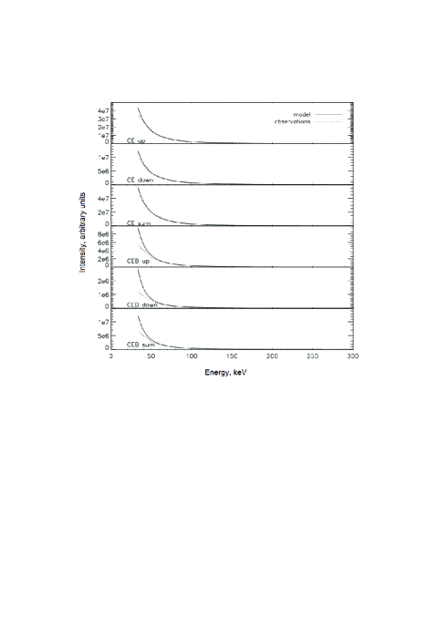
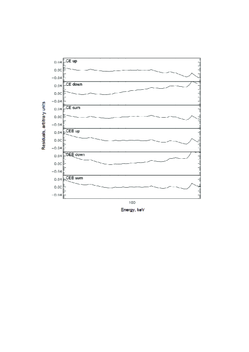
Figure 9: Comparison of the simulated upward, downward and total HXR intensities with the observations (left plots) and their residuals (right plots) calculated for different beam precipitation models (CE and CEB) and the viewing angle $180^{\circ}$ (along the magnetic field direction).

4.3.2 MW emission and polarization

Table 1: The $\chi^{2}$ statistics and significance coefficients for correlation between the observed and simulated MW intensities.

Points	${\chi}_{0}^{2}$	${\chi}_{0}^{2}$	Kendal	Spearman	${\chi}^{2}$	Kendal	Spearman	${\chi}^{2}$
of CEB	0.90	0.99	CEB3	CEB3	CEB3	CEB2	CEB2	CEB2
9	3.49	1.65	0.944	0.944	3.86	0.889	0.950	2.56
7	2.20	0.87	0.867	0.943	2.21	0.733	0.829	0.331
6	1.61	0.55	1.000	1.000	1.87	0.800	0.900	0.128
5	1.06	0.30	1.000	1.000	1.49	1.000	1.000	0.031

The distributions in frequency of MW emission and polarisation observed for this flare in 9 frequencies shown by asterisks were compared with the MW emission simulated with a radiative transfer approach in vertically stratified layers for different viewing angles (180, 140 and 110^∘) and for different electron precipitation models including collisions, electric field and magnetic field convergence as presented in Fig. 10 for a viewing angle of 140^∘ revealing the most reasonable agreement.

The observed MW spectrum was created by using the NoRP data plotted in Fig. 1a and the MW polarization variations were taken from the Fig. 1b. The MW emission simulated for optically thin plasma used for fitting the observations in the paper by Altyntsev et al. (2008) is presented on the plot by the dot-dashed line. The errors of MW emission measurements are shown by bars in Fig. 10. We calculated the standard deviation of the observed noise level ($\sigma$) for each frequency of MW observations by SBRS and NoRP. The errors in MW intensity and polarisation were estimated then from a sum of the statistical (3$\sigma$) and instrumental errors.

From a hydrodynamic model used to define the temperature and density variations with depth one can estimate the height of a semi-circular loop producing this flare to be about 10000 km. Then the distance between the MW and HXR intensity centroids can be estimated at about 10^′′ that fits very well the locations of MW and HXR contours.

The MW emission and polarisation simulated in section 4.2.2 by taking into account radiative transfer effects reveal smoother parts at medium and higher frequencies and a harmonic part at lower frequencies. The smooth part at higher frequencies has a negative power law close to that observed while for lower energy part it has a positive power law with a rather steep slope which is much higher than the one observed. In the current paper we are mostly concerned with the smooth part of MW emission and polarization simulated at higher frequencies for convergence of 2 and 3 (CEB2 and CEB3 and different viewing angles. While at lower frequencies we have accounted for Razin’s effect with the consideration of depth variations of the ambient density that improved the MW emission magnitude at lower frequencies. However, there are still some noticeable disagreements at very low frequencies between the observed and simulated MW emission as seen in Fig. 10 . These are possibly, related to the use of a simplified radiative transfer approach or some other effects which will require further investigation in the future.

For a viewing angle of 110^∘ , which in our model is equal to 70^∘ in the model by Altyntsev et al. (2008), the simulated MW intensity is not sensitive to the variations of the magnetic convergence factor and it is smaller than the observed one by more than 20$\%$ for both lower and higher frequencies. However, for a viewing angle of $140^{\circ}$ the model simulations of MW emission and polarization are able to reproduce very closely the main features of the observed MW emission. These include the magnitude and the frequency of MW emission maximum close to the ones observed; the frequency of the MW spectrum maximum appearing at about 17 GHz, a negative power law spectral index and a smooth decrease of MW emission towards lower frequencies with a spectral index about 2 (being still much higher than the observed one because of the simplified radiative transfer approach used and negative power law MW emission with the spectral index of 2.8 towards higher frequencies close to the observed one of 3).

The MW polarization simulated for models CEB2 and CEB3 for the same viewing angle of $140^{\circ}$ agrees with the observed polarisation at lower frequencies with CEB2 showing a closer agreement. Also the CEB2 model simulation of MW polarisation reproduces rather closely (9 GHz), within the limitations of our radiative transfer model, the observed frequency (7 GHz) of the polarisation reversal. While for higher frequencies the simulated polarisation is twice higher than the observations that can be the result of neglecting further scattering of MW emission on the ambient particles (Bastian 1995; Altyntsev et al. 1996), which can smoothen significantly a polarisation degree of MW emission at higher frequencies.

In order to quantify our fits in MW intensities, we carried out a few statistical tests for the likehood of each curves (CEB2 and observations, CEB3 and observations) by using the statistical SPSS package. The tests include Kendall tau and Spearman correlation tests (Isobe et al. 1986; Kendal & Gobbons 1990) appropriate for other than normal distributions which we have for MW emission. We also calculated $\chi^{2}$ coefficients (Chernoff & Lehmann 1954) for the following CEB2 and CEB3 sets: the full number of 9 measurements, for reduced 7 measurements (excluding the two points at lowest frequencies), then for 6 and 5 (reducing the measurements consequently by one from lower frequencies), in order to avoid the discrepancies in MW emission at the lowest frequencies. The results of these tests are presented in Table 1. For comparison, we also include the critical values of $\chi^{2}$ for given degrees of freedom corresponding to significance levels of 90$\%$ and 99$\%$.

It can be observed from Table 1 that the intensities for both models (CEB2 and CEB3) reveal strong positive correlation with MW observations for all 9 frequencies, but it increases to a full dependence (correlation coefficients approach 1.0) for the reduced number of measurements of 6 and 5 for CEB3 or 5 for CEB2. Although, for 9 points the correlation is slightly better for the model CEB2. The calculated $\chi^{2}$ for each datasets (CEB2 and CEB3) from the full to reduced measurement numbers plotted in Table 1 allow us to discriminate between the models. The model CEB3 produces $\chi^{2}$ of 3.86 for 9 points (or degree of freedom (DF) of 8) that is reduced to 1.49 for 5 points, or DF=4).

The $\chi^{2}$ coefficients for simulated and observed polarisation data obtained for 8 observational points (excluding 80 GHz), or 7 degrees of freedom, produced $\chi^{2}$=1.33 for model CEB2 and 2.13 for model CEB3 that reveals the similar close (above 95$\%$ fit to observations for the model with convergence 2 because their $\chi^{2}$ lie between the critical values for the confidence levels above 0.90 and below 0.99 (Chernoff & Lehmann 1954). This analysis of both MW intensity and polarisation allows to conclude that model simulations with any convergence fit reasonably well the MW observations up to the confidence level of 90$\%$. However, the model CEB2 with convergence 2 fits the observations up to 95$\%$ for all 9 points and up to the confidence level of 99$\%$ with a reduced number of 7 points and lower.

Therefore, it is safe to conclude that with the electron beam parameters derived from HXR emission, the best agreement with the MW observations at higher frequencies is achieved for CEB models with a reasonably small convergence factor of 2, the magnetic field magnitude at the photosphere derived from MDI (B = 780 G) and the viewing angle $140^{\circ}$ (see Fig. 10). The results of the simulations also allow us to estimate more accurately the inclination of the loop in the parts emitting the relevant types of emission: HXR or MW.

One can note that the observed MW emission from this flare better agrees with our simulated MW emission seen under the viewing angle of $140^{\circ}$, contrary to the viewing angle of $80^{\circ}$(equal to 100^∘ in the current model) deduced in the earlier simulations (Altyntsev et al. 2008) and to the angle of $180^{\circ}$ obtained for HXR emission in the current paper. As we discussed above, the difference between the viewing angles derived for MW emission from our models and those by Altyntsev et al. (2008) can be a result of the over-simplified model used in the latter and a limited number of measurements.

Figure 10: Comparison of observed MW intensity in solar flux units (sfu)(top plot) and degree of polarization (bottom plot) with results of the simulations with CEB2 model for a magnetic field convergence of 2 (dotted line curves) and CEB3 model with convergence of 3 (solid line curves) and the model presented by Altyntsev et al. (2008) (dash-dotted line). In the both plots asterisks mark the observed spectra.

However, the difference between MW and HXR viewing angles found in the current paper can be explained within our model by the assumption that the flaring loop was not standing perpendicular to the local horizontal plane in the flare location but was slightly tilted (by about $40^{\circ}$) towards the solar disk center. By comparing the directivity of MW and HXR emission from Fig. 14 one can observe that the MW emission has the preferential direction of 30^∘ downwards and of 130-140^∘ upwards.

The downward emission exceeds by factor 2-4 the upward emission. If all these downward photons are fully reflected by the photosphere (albedo effect) with the same properties (angles and energies) they can contribute to reasonable fit of MW emission for the viewing angle of 140^∘ compared to 180^∘ from HXR spectra, e.g. this difference in viewing angles can be just a result of the directivity effects on HXR and MW intensity from beam electrons. One can also speculate that the loop curvature in the observed flare could contribute to this angle difference for viewing MW and HXR emission to confirm which one needs to extend our model to semi-circular loop that can be done in the future.

5 Conclusions

In this paper for the first an attempt is made to simulate HXR and MW emission and polarisation emitted from he flare of 10 March 2001 with the same population of electrons, in order to improve the fit of observations reported in previous studies. This is achieved by applying the Fokker–Planck kinetic approach to precipitation of electron beam with energy range from 12 keV to 10 MeV into a converging magnetic loop with anisotropic electron scattering on the ambient particles in Coloumb collisions and Ohmic losses. The theoretical HXR and MW emissions are then calculated by using these distribution functions for different factors of magnetic field convergence and viewing angles as described in our previous papers (Zharkova et al. 2010; Kuznetsov & Zharkova 2010).

The observed HXR photon spectra and frequency distribution of MW emission and polarisation reveal the best fit for the FP models including the effect of electric field induced by beam electrons precipitating in a converging magnetic loop. Magnetic field strengths in the footpoints on the photosphere were updated with newly calibrated SOHO/MDI data. The observed HXR energy spectrum is shown to be a double power law which was fit very closely by the photon spectrum simulated for the models including the self-induced electric field.

The MW emission simulated for different models was compared with the observed distribution in frequency revealing that only the models combining collisions and electric field effects with pitch angle anisotropy were able to reproduce closely the main features of the observed MW emission: peak magnitude and frequency, a negative spectral index of 2.8 versus 3 observed for higher frequencies, a smoother decrease of MW emission towards lower frequencies and the correct frequency of the MW polarisation reversal. There are still disagreements between simulated and MW emission observed at lower frequencies which are likely to be caused by simplified model of radiative transfer considered in the current approach and by not taking into account the emission from the ambient electrons in a vicinity of the flare.

By estimating from the hydrodynamic model the height of a semi-circular loop to be about 10000 km and by taking into account the inclination of the loop in HXR emission, the distance between the MW and HXR intensity centroids was about 10^′′ that agrees rather well the observations.

HXR emission simulated for relativistic angle-dependent cross-section accounting for different directions of electron propagation (downwards and upwards) reveal that in the corona the majority of electrons moves in the downward direction with a twice smaller number moving upwards while in the chromosphere most electrons move upwards and only smaller fraction keeps moving downwards. Thus, for this flare the effects of electron’s magnetic mirroring and Ohmic losses were significant.

The observed HXR spectrum reveals a noticeable flattening towards lower energies below 50 keV indicating a significant effect of the self-induced electric field in beam electron energy losses. The observed HXR photon spectrum was best fit by the model simulated for collisional plus Ohmic losses (CE) precipitation model of electron beam with the initial energy flux of $10^{12}$ erg/s/cm² and spectral index about 3 including the emission emitted upwards and downwards (the full albedo effect) in the direction of $180^{\circ}$ (towards the magnetic field direction) that for this flare location indicates a loop tilt about 40^∘ towards the solar disk centre.

The observed MW emission distribution in frequency reveals a better fit for the model combining collisions and electric field effects with a moderate magnetic field convergence of 2 (CEB2). This electron precipitation model can reproduce closely within better than $90\%$ confidence level for all 9 points of observations and up to $95\%$ confidence level for 6 points excluding the three ones at lowest frequencies) the main features in the observed MW emission: the maximum magnitude and the frequency at about 17 GHz, a smooth decrease of MW emission towards lower frequencies with a spectral index about 2, the spectral index of 2.8 for higher energy part of MW emission and the frequency of reversal of MW polarisation.

The both models CEB2 and CEB3 show a reasonable fit to the observed polarisation magnitudes; although the model CEB2 shows a better fit to the frequency of the MW polarisation reversal close to the observed one within the $90\%$ confidence level for all 9 points of observations and up to $95\%$ confidence level for 6 points excluding the three observations at lowest frequencies.

In this study the closest fit for observed MW emission was achieved for the simulations with a weakly (factor 2) converging magnetic field seen at the viewing angle of $140^{\circ}$, contrary to 80^∘ (corresponding to 100^∘ in our model) derived previously (Altyntsev et al. 2008). While for HXR emission the closest agreement between observed and simulated photon spectra was obtained for the model with collisions and electric field only with the emission seen at $180^{\circ}$ (from the loop top).

Within the limitations of our radiative transfer model, this difference is likely to reflect, at first, the inclination of about 40^∘ of the flaring loop towards the solar disk centre that accounts for the HXR viewing angle. At second, this difference can also indicate a difference in the preferential directivity of HXR and MW emission caused by electron scattering effects in a presence of self-induced electric and converging magnetic fields. In addition, a flaring loop curvature in the upper atmosphere where the MW emission is formed can also contribute to this viewing angle difference.