1. Introduction

This paper describes an efficient technique for solving Poisson problems defined on the integer lattice $\mathbb{Z}^{2}$. For simplicity of presentation, we limit our attention to the equation

(1.1) $$[\mathsf{A}u](\bm{m})=f(\bm{m}),\qquad\bm{m}\in\mathbb{Z}^{2},$$

where $f=f(\bm{m})$ and $u=u(\bm{m})$ are scalar valued functions on $\mathbb{Z}^{2}$, and where $\mathsf{A}$ is the so-called discrete Laplace operator

(1.2) $$[\mathsf{A}\,u](\bm{m})=4u(\bm{m})-u(\bm{m}+\bm{e}_{1})-u(\bm{m}-\bm{e}_{1})-u(\bm{m}+\bm{e}_{2})-u(\bm{m}-\bm{e}_{2}),\qquad\bm{m}\in\mathbb{Z}^{2}.$$

In (1.2), $\bm{e}_{1}=[1,0]$ and $\bm{e}_{2}=[0,1]$ are the canonical basis vectors in $\mathbb{Z}^{2}$. If $f\in L^{1}(\mathbb{Z}^{2})$ and $\sum_{\bm{m}\in\mathbb{Z}^{2}}|f(\bm{m})|=0$, equation (1.1) is well-posed when coupled with a suitable decay condition for $u$, see [19] for details.

We are primarily interested in the situation where the given function $f$ (the source) is supported at a finite number of points which we refer to as source locations, and where the function $u$ (the potential) is sought at a finite number of points called target locations. While the solution technique is described for the equation (1.1) involving the specific operator (1.2), it may readily be extended to a broad range of lattice equations involving constant coefficient elliptic difference operators.

Variations of the equation (1.1) are perhaps best known as a set of equations associated with the discretization of elliptic partial differential equations. However, such equations also emerge in their own right as natural models in a broad range of applications: random walks [9], analyzing the Ising model (in determining vibration modes of crystals), and many others in engineering mechanics including micro-structural models, macroscopic models, simulating fractures [23, 16] and as models of periodic truss and frame structures [6, 25, 19, 24].

Of particular interest in many of these applications is the situation where the lattice involves local deviations from perfect periodicity due to either broken links, or lattice inclusions. The fast technique described in this paper can readily be modified to handle such situations, see Section 10.1. It may also be modified to handle equations defined on finite subsets of $\mathbb{Z}^{2}$, with appropriate conditions (Dirichlet / Neumann / periodic) prescribed on the boundary, see Section 10.2 and [10].

The technique described is a descendant of the Fast Multipole Method (FMM) [12, 13, 14], and, more specifically, of “kernel independent” FMMs [11, 21, 26]. A key application of the original FMM was to rapidly solve the Poisson equation

(1.3) $$-\Delta u(\bm{x})=f(\bm{x}),\qquad\bm{x}\in\mathbb{R}^{2},$$

which is the continuum analog of (1.1). The FMM exploits the fact that the analytic solution to (1.3) takes the form of a convolution

(1.4) $$u(\bm{x})=\int_{\mathbb{R}^{2}}\phi_{\rm cont}(\bm{x}-\bm{y})\,f(\bm{y})\,d\bm{y},$$

where $\phi_{\rm cont}$ is the fundamental solution of the Laplace operator,

(1.5) $$\phi_{\rm cont}(\bm{x})=-\frac{1}{2\pi}\log|\bm{x}|.$$

If the source function $f$ corresponds to a number of point charges $\{q_{j}\}_{j=1}^{N}$ placed at locations $\{\bm{x}_{j}\}_{j=1}^{N}$, and if the potential $u$ is sought at same set of locations, then the convolution (1.4) simplifies to the sum

(1.6) $$u_{i}=\underset{j\neq i}{\sum_{j=1}^{N}}\phi_{\rm cont}(\bm{x}_{i}-\bm{x}_{j})\,q_{j},\qquad i=1,\,2,\,\dots,\,N.$$

While direct evaluation of (1.6) requires $O(N^{2})$ operations since the kernel is dense, the FMM constructs an approximation to the potentials $\{u_{i}\}_{i=1}^{N}$ in $O(N)$ operations. Any requested approximation error $\varepsilon$ can be attained, with the constant of proportionality in the $O(N)$ estimate depending only logarithmically on $\varepsilon$.

In the same way that the FMM can be said to rely on the fact that the Poisson equation (1.3) has the explicit analytic solution (1.4), the techniques described in this paper can be said to rely on the fact that the lattice Poisson equation (1.1) has an explicit analytic solution in the form

(1.7) $$u(\bm{m})=[\phi*f](\bm{m})=\sum_{\bm{n}\in\mathbb{Z}^{2}}\phi(\bm{m}-\bm{n})\,f(\bm{n}).$$

where $\phi$ is a fundamental solution for the discrete Laplace operator (1.2). This fundamental solution is known analytically [7, 19, 20, 10] via the normalized Fourier integral

(1.8) $$\phi(\bm{m})=\frac{1}{(2\,\pi)^{2}}\int_{-\pi}^{\pi}\int_{-\pi}^{\pi}\frac{\cos(t_{1}m_{1}+t_{2}m_{2})-1}{4\,\sin^{2}(t_{1}/2)+4\,\sin^{2}(t_{2}/2)}\,dt_{1}\,dt_{2},\qquad\bm{m}=[m_{1},\,m_{2}]\in\mathbb{Z}^{2}.$$

This paper presents an adaptation of the original Fast Multipole Method that enables it to handle discrete kernels such as (1.8) and to exploit accelerations that are possible due the geometric restrictions present in the lattice case. The method extends directly to any problem that can be solved via convolution with a discrete fundamental solution. The technique for numerically evaluating (1.8) extends directly to other kernels, see Section 3.

While we are not aware of any previously published techniques for rapidly solving the free space problem (1.1) (or, equivalently, for evaluating (1.7)), there exist very fast solvers for the closely related case of lattice Poisson equations defined on rectangular subsets of $\mathbb{Z}^{2}$ with periodic boundary conditions. Such equations become diagonal when transformed to Fourier space, and may consequently be solved very rapidly via the FFT. The computational time $T_{\rm fft}$ required by such a method satisfies

(1.9) $$T_{\rm fft}\sim N_{\rm domain}\log N_{\rm domain}\qquad\mbox{as}\ N_{\rm domain}\rightarrow\infty,$$

where $N_{\rm domain}$ denotes the number of lattice nodes in the smallest rectangular domain holding all source locations, and where the constant of proportionality is very small. Similar complexity, sometimes without the logarithmic factor, and with fewer restrictions on the boundary conditions, may also be achieved via multigrid methods [3].

The principal contribution of the present work is that the computational time $T_{\rm FMM}$ required by the method described here has asymptotic complexity

(1.10) $$T_{\rm FMM}\sim N_{\rm sources},\qquad\mbox{as}\ N_{\rm sources}\rightarrow\infty,$$

where $N_{\rm sources}$ denotes the number of lattice nodes that are loaded (assuming that the solution is sought only at the source points). In a situation where the source points are relatively densely distributed in a rectangle, we would have $N_{\rm domain}\approx N_{\rm sources}$ and there would be no point in using the new method (in fact, an FFT based method is in this case significantly faster since the constant of proportionality in (1.9) is smaller than that in (1.10)). However, if the source and target points are relatively sparsely distributed in the lattice, then the estimate (1.10) of the new method is clearly superior to that of (1.9) for an FFT based method. As demonstrated in Section 9, very significant gains in speed can be achieved. Perhaps even more importantly, much larger problems can be handled since an FFT based method requires that the potential on all $N_{\rm domain}$ nodes be held in memory.

• Example: The distinction between $N_{\rm domain}$ in (1.9) and $N_{\rm sources}$ in (1.10) can be illustrated with the toy example shown in Figure 1.1. The figure illustrates a portion of an infinite lattice in which $N_{\rm source}=11$ nodes have been loaded. A rectangular domain covering these loads is marked with a blue dashed line and holds $N_{\rm domain}=80$ nodes. Clearly $N_{\rm sources}=11\ll 80=N_{\rm domain}$. A solution strategy for (1.1) based on the FFT or multigrid would involve all $N_{\rm domain}$ nodes inside the rectangle. In contrast, the lattice fundamental solution allows the solution task to be reduced to evaluating the sum (1.7) which involves an $N_{\rm sources}\times N_{\rm sources}$ dense coefficient matrix.

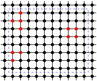
Figure 1.1. A subset of the infinite lattice $\mathbb{Z}^{2}$. The $N_{\rm sources}=11$ red nodes are loaded. The smallest rectangle holding all sources is marked with a dashed blue line. It has $N_{\rm domain}=80$ nodes.

2. Review of fast summation techniques

In this section, we briefly outline the basic ideas behind the Fast Multipole Method, and then describe the modifications required to evaluate a lattice sum such as (1.7). Our presentation assumes some familiarity with Fast Multipole Methods; for an introduction, see, e.g., [2, 13]. As a model problem, we consider the task of evaluating the sum

(2.1) $$u_{i}=\sum_{j=1}^{N}\phi(\bm{x}_{i}\,-\,\bm{x}_{j})\,q_{j},$$

where $\{\bm{x}_{i}\}_{i=1}^{N}$ is a set of $N$ points in the plane, where $\{q_{i}\}_{i=1}^{N}$ is a set of $N$ given real numbers called charges, where $\{q_{i}\}_{i=1}^{N}$ is a set of $N$ sought real numbers called potentials, and where $\phi\,\colon\,\mathbb{R}^{2}\times\mathbb{R}^{2}\rightarrow\mathbb{R}$ is a kernel function.

Figure 2.1. Geometry of the $N$-body problem in Section 2. Source $i$ is blue, the sources in $J_{i}^{\rm near}$ as defined by (2.3) are red.

For simplicity, we consider in this review only the case where the sources are more or less uniformly distributed in a computational box $\Omega$ in the sense that $\Omega$ can be split into equi-sized small boxes, called leaves, in such a way that each small box holds about the same number of sources. We let $N_{\rm leaf}$ denote an upper bound for the number of sources held in any leaf. Then the sum (2.1) can be split into two parts

$$u_{i}=u^{\rm near}_{i}+u^{\rm far}_{i},$$

where the near-field is defined by

(2.2) $$u^{\rm near}_{i}=\sum_{j\in J_{i}^{\rm near}\backslash\{i\}}\phi(\bm{x}_{i}-\bm{x}_{j})\,q_{j},\qquad i=1,\,2,\,\dots,\,N,$$

where $J_{\rm i}^{\rm near}$ is an index list marking all sources that lie either in the same box as charge $i$, or in a box that is directly adjacent to the box holding source $i$,

(2.3) $$J_{i}^{\rm near}=\{j\,\colon\,\bm{x}_{i}\mbox{ and }\bm{x}_{j}\mbox{ are located in the same leaf or in directly adjacent leaves}\}.$$

The definition of $J_{i}^{\rm near}$ is illustrated in Figure 2.1. The far-field is then defined by

(2.4) $$u^{\rm far}_{i}=\sum_{j\notin J_{i}^{\rm near}}\phi(\bm{x}_{i}-\bm{x}_{j})\,q_{j},\qquad i=1,\,2,\,\dots,\,N,$$

The near-field (2.2) can now be directly evaluated at low cost since at most $9\,N_{\rm leaf}$ sources are near any given source. In the lattice case, this step could potentially be rendered expensive by the fact that the kernel is known only via the Fourier integral (1.8) which is quite costly to evaluate via quadrature. We describe in Section 3 how this step may be accelerated by pre-computing and storing the values of $\phi(\bm{m})$ for all small values of $\bm{m}$ and then using an asymptotic expansion for large $\bm{m}$. We observe that the local evaluation gets particularly effective whenever the number of lattice cells along the side of any leaf box is bounded by some fixed number $L$ of moderate size (say $L\leq 1000$). In this case, there is in the lattice situation only $16\,L^{2}$ possible relative positions of two charges that are near each other which means that evaluation of the kernel for the near-field calculations amounts to simply a table lookup. (In fact, due to symmetries, only $2\,L^{2}$ values need to be stored.)

The far-field (2.4) is as in the classical FMM evaluated via the computation of so-called multipole expansions and incoming expansions. These in turn are constructed via a hierarchical procedure on a quad-tree such as the one shown in Figure 6.1. With the development of so-called kernel independent FMMs, the multipole expansions of the original FMM were superseded by more general representations valid for a broad range of kernels. The bulk of this paper consists of a description of such a kernel independent FMM, adapted to exploit geometrical restrictions imposed in the lattice case. Section 4 reviews a technique for compactly representing charges and potentials, and Section 5 describes how it can be adapted to the particular case of lattice equations. Section 6 introduces notation for handling quad-trees, Section 7 describes the so-called translation operators, then the full lattice FMM is described in Section 8.

3. Evaluation of the lattice fundamental solution

The numerical evaluation of the function $\phi$ in (1.8) requires some care since the integrand has a singularity at the origin and gets highly oscillatory when $|\bm{m}|$ is large. The latter issue can be handled quite easily since a highly accurate asymptotic expansion of $\phi(\bm{m})$ as $|\bm{m}|\rightarrow\infty$ is known, see Section 3.1. When $|\bm{m}|$ is small, quadrature and Richardson extrapolation may be used to compute $\phi(\bm{m})$ to very high accuracy, see Section 3.2. We note that in the regime where $|\bm{m}|$ is small, there is only a limited number of possible values of $\bm{m}$, and the corresponding values of $\phi(\bm{m})$ can be pre-computed and stored. Consequently, evaluating $\phi(\bm{m})$ in the near-field amounts simply to a table look-up, which is very fast.

3.1. Evaluation of fundamental solution for $|\bm{m}|$ large

It has been established (see e.g. [7, 8, 18, 19, 20]) that as $|\bm{m}|\rightarrow\infty$, the fundamental solution $\phi$ defined by (1.8) has the asymptotic expansion

(3.1) $$\phi(\bm{m})=-\frac{1}{2\pi}\left(\log|\bm{m}|+\gamma+\frac{\log 8}{2}\right)+\frac{1}{24\pi}\frac{m_{1}^{4}-6m_{1}^{2}m_{2}^{2}+m_{2}^{4}}{|\bm{m}|^{6}}\\ +\frac{1}{480\pi}\frac{43m_{1}^{8}-772m_{1}^{6}m_{2}^{2}+1570m_{1}^{4}m_{2}^{4}-772m_{1}^{2}m_{2}^{6}+43m_{2}^{8}}{|\bm{m}|^{12}}+O(1/|\bm{m}|^{6}).$$

The number $\gamma$ is the Euler constant ($\gamma=0.577206\cdots$).

For $|\bm{m}|$ large, we approximate $\phi$ by dropping the $O(1/|\bm{m}|^{6})$ term off the asymptotic expansion. We found that for $|\bm{m}|>30$ the expansion (3.1) is accurate to at least $10^{-12}$.

The asymptotic expansion (3.1) is valid for the simple square lattice only. However, there is a simple process for constructing analogous expansions for fundamental solutions associated with a very broad class of constant coefficient elliptic difference operators [20]. The process can be automated and executed using symbolic software such as Maple [19].

3.2. Evaluation of fundamental solution for $|\bm{m}|$ small

When $|\bm{m}|$ is small enough that the asymptotic expansion provides insufficient accuracy, we approximate the integral (1.8) using a two-step quadrature procedure: First, the domain $[-\pi,\,\pi]^{2}$ is split into $n\times n$ equisized boxes where $n$ is an odd number chosen so that each box holds about one oscillation of the integrand (in other words, $n\approx|\bm{m}|$). For each box not containing the origin, the integral is approximated using a Cartesian Gaussian quadrature with $20\times 20$ nodes. This leaves us with the task of evaluating the integral

$$g(a)=\frac{1}{(2\,\pi)^{2}}\int_{-a}^{a}\int_{-a}^{a}\frac{\cos(t_{1}m_{1}+t_{2}m_{2})-1}{4\,\sin^{2}(t_{1}/2)+4\,\sin^{2}(t_{2}/2)}\,dt_{1}\,dt_{2},$$

where $a=\pi/n$ denotes the size of the center box. Now observe that

(3.2) $$g(a)=\sum_{n=0}^{\infty}\left(g\left(\frac{a}{2^{n}}\right)-g\left(\frac{a}{2^{n+1}}\right)\right)=\sum_{n=0}^{\infty}\frac{1}{(2\,\pi)^{2}}\int_{\Omega_{n}}\frac{\cos(t_{1}m_{1}+t_{2}m_{2})-1}{4\,\sin^{2}(t_{1}/2)+4\,\sin^{2}(t_{2}/2)}\,dA,$$

where

$$\Omega_{n}=[2^{-n}\,a,\,2^{-n}\,a]^{2}\backslash[2^{-n-1}\,a,\,2^{-n-1}\,a]^{2},\qquad n=1,\,2,\,3,\,\dots$$

is a sequence of annular domains whose union is the square $[-a,\,a]^{2}$. All integrals in (3.2) involve non-singular integrands, and can easily be evaluated via Gaussian quadratures. (We split each $\Omega_{n}$ into eight rectangular regions and use a $20\times 20$ point Gaussian quadrature on each.) Using Richardson extrapolation to accelerate the convergence, it turns out that only about 14 terms are needed to evaluate the sum (3.2) to a precision of $10^{-14}$.

Remark 3.1.

The particular integral (1.8) can be evaluated via a short-cut since it is possible to evaluate the integral over $t_{1}$ analytically, and then use quadrature only for the resulting (non-singular) integral over $t_{2}$, see [19]. Similar tricks are likely possible in many situations involving mono-atomic lattices. However, we prefer to not rely on this approach since it does not readily generalize to vector valued problems (such as those associated with mechanical lattice problems) or multi-atomic lattices.

4. Outgoing and incoming expansions

In this section, we present techniques for efficiently approximating the far-field $u^{\rm far}_{i}$ to any given positive precision $\varepsilon$. The parameter $\varepsilon$ can be tuned to balance the computational cost verses the accuracy. In the numerical examples reported in Section 9, $\varepsilon=10^{-10}$.

4.1. Interaction ranks

An essential component of the classical FMM is an efficient technique for representing potentials and source distributions via “expansions” of different kinds. To illustrate the concept, let us consider a simplified problem in which a number of sources are placed in a “source box” $\Omega_{\tau}$, and the potential induced by these sources is to be evaluated at a number of locations in a “target box” $\Omega_{\rm\sigma}$. The orientation of the boxes is shown in Figure 4.1. To be precise, we suppose that sources $\{q_{j}^{\tau}\}_{j=1}^{N}$ are placed at locations $\{\bm{x}_{j}^{\tau}\}_{j=1}^{N}\subset\Omega_{\rm\tau}$, and that we seek the potentials $\{u_{i}^{\sigma}\}_{i=1}^{M}$ induced at some locations $\{\bm{x}_{i}^{\sigma}\}_{i=1}^{M}\subset\Omega_{\rm\sigma}$,

(4.1) $$u_{i}^{\sigma}=\sum_{j=1}^{N}\Phi(\bm{x}_{i}^{\sigma},\,\bm{x}_{j}^{\tau})\,q_{j}^{\tau},\qquad i=1,\,2,\,\dots,\,M.$$

In this review of the classical FMM, the kernel $\Phi$ is defined by

$$\Phi(\bm{x},\bm{y})=\phi_{\rm cont}(\bm{x}-\bm{y})=-\frac{1}{2\pi}\log|\bm{x}-\bm{y}|,$$

where $\phi_{\rm cont}$ is the fundamental solution of the Laplace equation. For convenience, we write (4.1) as a matrix-vector product

(4.2) $$\bm{u}^{\sigma}=\mathsf{A}^{\sigma,\tau}\,\bm{q}^{\tau},$$

where $\bm{u}^{\sigma}=[u_{i}^{\sigma}]_{i=1}^{M}$ and $\bm{q}^{\tau}=[q_{j}^{\tau}]_{j=1}^{N}$, and where $\mathsf{A}^{\sigma,\tau}$ is the $M\times N$ matrix with entries

$$\mathsf{A}_{ij}^{\sigma,\tau}=\Phi(\bm{x}_{i}^{\sigma},\,\bm{x}_{j}^{\tau}).$$

Figure 4.1. Illustration of source box $\Omega_{\tau}$ and target box $\Omega_{\sigma}$.

A key observation underlying the FMM is that to any finite precision $\varepsilon$, the rank of a matrix such as $\mathsf{A}^{\sigma,\tau}$ is bounded independently of the numbers $M$ and $N$ of targets and sources in the two boxes. In fact, the $\varepsilon$-rank $P$ of $\mathsf{A}^{\sigma,\tau}$ satisfies

$$P\lesssim\log(1/\varepsilon),\quad\mbox{as}\ \varepsilon\rightarrow 0.$$

The constant of proportionality depends on the geometry of the boxes, but is typically very modest. As a consequence of this rank deficiency, it is possible to factor the matrix $\mathsf{A}^{\sigma,\tau}$, say

(4.3) $$\begin{array}[]{ccccccc}\mathsf{A}^{\sigma,\tau}&\approx&\mathsf{B}&\mathsf{C},\\ M\times N&&M\times P&P\times N\end{array}$$

and then to evaluate the potential $\bm{u}^{\tau}$ in two steps:

(4.4) $$\bm{v}=\mathsf{C}\,\bm{q}^{\tau},\qquad\bm{u}\approx\mathsf{B}\,\bm{v}.$$

The cost of evaluating $\bm{u}$ via (4.4) is $O((M+N)\,P)$, which should be compared to the $O(M\,N)$ cost of evaluating $\bm{u}$ via (4.2).

4.2. Formal definitions of outgoing and incoming expansions

In the classical FMM, a “multipole expansion” for a box is a short vector from which the potential caused by all charges in the box can be evaluated; it can be viewed as a compressed representation of all the charges inside the box. In this section, we introduce the “outgoing expansion” as a generalization of this idea that allows representations other than classical multipole expansions to be incorporated. The “incoming expansion” is analogously introduced to generalize the concept of a “local expansion.”

Well-separated boxes: Let $\Omega$ be a box with side length $2a$ and center $\bm{c}$ as shown in Figure 4.2. We say that a point $\bm{x}$ is well-separated from $\Omega$ if it lies outside the square of side length $6a$ centered at $\bm{c}$. We say that two boxes $\Omega$ and $\Omega^{\prime}$ are well-separated if every point in $\Omega^{\prime}$ is well-separated from $\Omega$, and vice versa.

Outgoing expansion: Let $\Omega$ be a box containing a set of sources. We say that a vector $\hat{\bm{q}}$ is an outgoing expansion for $\Omega$ if the potential caused by the sources in $\Omega$ can be reconstructed from $\hat{\bm{q}}$ to within precision $\varepsilon$ at any point that is well-separated from $\Omega$.

Incoming expansion: Let $\Omega$ be a box in which a potential has been induced by a set of sources located at points that are well-separated from $\Omega$. We say that a vector $\bm{\hat{u}}$ is an incoming expansion for $\Omega$ if $u$ can be reconstructed from $\hat{\bm{u}}$ to within precision $\varepsilon$.

Figure 4.2. Illustration of well-separated points. Any point on or outside of the dashed square is well-separated from $\Omega$. Consequently, the points $\bm{x}_{2}$, $\bm{x}_{3}$, and $\bm{x}_{4}$ are well-separated from $\Omega$, but $\bm{x}_{1}$ is not.

4.3. Charge basis

The cost of computing a factorization such as (4.3) using a generic linear algebraic technique such as QR is $O(M\,N\,P)$, which would negate any savings obtained when evaluating the matrix-vector product (unless a very large number of matrix-vector products involving the same source and target locations is required). Fortunately, it is possible in many environments to construct such factorizations much faster. The classical FMM uses multipole expansions. As an alternative, an approach based on so-called “proxy charges” has recently been developed [26]. It has been demonstrated [21, 22] that for any given box $\Omega$, it is possible to find a set of locations $\hat{\bm{Y}}=\{\hat{\bm{y}}_{p}\}_{p=1}^{P}\subset\Omega$ with the property that sources placed at these points can to high accuracy replicate any potential caused by a source distribution in $\Omega$. The number of points $P$ required is given in Table 1. To be precise, given any set of points $\bm{Y}=\{\bm{y}_{j}\}_{j=1}^{N}\subset\Omega$ and any sources $\bm{q}=\{q_{j}\}_{j=1}^{N}$, we can find “equivalent charges” $\hat{\bm{q}}=\{\hat{q}_{p}\}_{p=1}^{P}$ such that

(4.5) $$\sum_{j=1}^{N}\phi_{\rm cont}(\bm{x}\,-\,\bm{y}_{j})\,q_{j}\approx\sum_{p=1}^{P}\phi_{\rm cont}(\bm{x}\,-\,\hat{\bm{y}}_{p})\,\hat{q}_{p},$$

whenever $\bm{x}$ is well-separated from $\Omega$. The approximation (4.5) holds to some preset (relative) precision $\varepsilon$. Moreover, the map from $\bm{q}$ to $\hat{\bm{q}}$ is linear, and there exists a matrix $\mathsf{T}_{\rm ofs}=\mathsf{T}_{\rm ofs}(\hat{\bm{Y}},\,\bm{Y})$ such that

(4.6) $$\hat{\bm{q}}=\mathsf{T}_{\rm ofs}\,\bm{q},$$

where “ofs” is an abbreviation of “outgoing [expansion] from sources.”

	$\epsilon$
$l$	$10^{-6}$	$10^{-8}$	$10^{-10}$	$10^{-13}$
$1/32$	$19$	$27$	$37$	$49$
$1/16$	$19$	$27$	$36$	$49$
$1/4$	$19$	$28$	$37$	$49$
$1/2$	$21$	$29$	$37$	$51$

Table 1. The number of points $P$ required to replicate the field to accuracy $\epsilon$ for a box $\Omega$ with side length $l$.

We say that the points $\{\hat{\bm{y}}_{p}\}_{p=1}^{P}$ form an outgoing skeleton for $\Omega$, and that the vector $\hat{\bm{q}}$ is an outgoing expansion of $\Omega$.

In addition, we can find an incoming skeleton $\hat{\bm{X}}=\{\hat{\bm{x}}_{p}\}_{p=1}^{P}\subset\Omega$ with the property that any incoming potential in $\Omega$ can be interpolated from its values on the incoming skeleton. To be precise, suppose that $U=U(\bm{x})$ is a potential caused by sources that are well-separated from $\Omega$, and that $\bm{X}=\{\bm{x}_{i}\}_{i=1}^{M}$ is an arbitrary set of points in $\Omega$. Then there exists a matrix $\mathsf{T}_{\rm tfi}=\mathsf{T}_{\rm tfi}(\bm{X},\hat{\bm{X}})$ (‘tfi” stands for “targets from incoming [expansion]”) such that

$$\bm{u}=\mathsf{T}_{\rm tfi}\,\hat{\bm{u}},$$

where

$$\bm{u}=[U(\bm{x}_{i})]_{i=1}^{M},\qquad\mbox{and}\qquad\hat{\bm{u}}=[U(\hat{\bm{x}}_{p})]_{p=1}^{P}.$$

When the kernel $\Phi$ is symmetric in the sense that $\Phi(\bm{x}\,-\,\bm{y})=\Phi(\bm{y}\,-\,\bm{x})$ for all $\bm{x}$ and $\bm{y}$, any outgoing skeleton is also an incoming skeleton,

$$\hat{\bm{X}}=\hat{\bm{Y}}.$$

Moreover, if the target points equal the source points so that $\bm{X}=\bm{Y}$, then

$$\mathsf{T}_{\rm tfi}=\left(\mathsf{T}_{\rm ofs}\right)^{*}.$$

Applied to the situation described in Section 4.1, where a set of sources were placed in a source box $\Omega_{\tau}$, and we sought to evaluate the potential induced at a set of target points in a box $\Omega_{\sigma}$, the claims of this section can be summarized by saying that $\mathsf{A}^{\sigma,\tau}$ admits an approximate factorization

$$\begin{array}[]{ccccccc}\mathsf{A}^{\sigma,\tau}&\approx&\mathsf{T}_{\rm tfi}^{\sigma}&\mathsf{T}_{\rm ifo}^{\sigma,\tau}&\mathsf{T}_{\rm ofs}^{\tau}\\ M\times N&&M\times P&P\times P&P\times N\end{array}$$

where the middle factor is simply a subsampling of the original kernel function

$$\mathsf{T}_{\mbox{ifo},pq}^{\sigma,\tau}=\Phi(\hat{\bm{x}}_{p}^{\sigma},\,\hat{\bm{x}}_{q}^{\tau}).$$

Remark 4.1.

For solving multiple problems involving different source and load distributions that involve the same kernel, one set of skeleton points may be used for all problems by choosing the skeleton points to lie on the boundary of $\Omega_{\sigma}$ and $\Omega_{\tau}$. The interpolation matrices $\mathsf{T}_{\rm tfi}$ and $\mathsf{T}_{\rm ofs}$ need be constructed for each unique set of source and load distributions using the techniques from [5]. In Section 5, we describe this generalization of the skeletonization process in more detail for the lattice fundamental solution.

5. Constructing charge bases for the lattice fundamental solution

In this section, we describe how to construct the charge bases for the lattice fundamental solution defined by (1.8).

From potential theory, we know that to capture the interaction between a set of source points $\{\bm{m}^{\tau}_{j}\}_{j=1}^{N}$ in box $\Omega_{\tau}$ and all points far from $\Omega_{\tau}$, it is enough to capture the interaction between the source points and a set of “proxy” points $F$ that lie densely on the boundary of a box that is concentric to $\Omega_{\tau}$ and has a boundary that is well-separated from $\Omega_{\tau}$.

We choose the skeleton points to be a subset of the set of all points $Y$ that lie on the boundary of box $\tau$. Either rank revealing QR factorization [15] or factorization techniques from [5] are applied to the matrix $\mathsf{A}^{F,Y}$ (whose entries are given by $\mathsf{A}^{F,Y}_{i,j}=\Phi(\bm{m}_{i}^{F}\,-\,\bm{m}_{j}^{Y})$) to determine the rank $P$ and which $P$ points make up the set of skeleton points $\hat{Y}$ of $\Omega_{\tau}$.

Using the skeleton points and the techniques from [5], we find the $P\times N$ matrix $\mathsf{T}_{\rm{ofs}}$ such that

(5.1) $$\|\mathsf{A}^{F,\tau}-\mathsf{A}^{F,\hat{Y}}\mathsf{T}_{\rm{ofs}}\|<\epsilon.$$

We use a similar technique to find the incoming skeleton points and the translation operator $\mathsf{T}_{\rm{tfi}}$.

Remark 5.1.

Because of the smoothness of the kernel, it is not required to use all the points on the boundary of the well-separated box as “proxy” points. We found it is enough to take 40 points per edge to approximate the far field with accuracy $10^{-10}$.

6. Tree structure

The separation of variables in the kernel that was described in Section 4 is all that is needed to effectively evaluate a potential field whenever the set of target locations is well-separated from the set of source locations. When the two sets coincide, we need to tessellate the box containing them into smaller boxes, and use the expansion only for interactions between boxes that are well-separated. In this section, we describe the simplest such tessellation.

Suppose that we are given a set of points $\{\bm{x}_{i}\}_{i=1}^{N}$ in a box $\Omega$. Given an integer $N_{\rm leaf}$, we pick the smallest integer $L$ such that when the box $\Omega$ is split into $4^{L}$ equisized smaller boxes, no box holds more than $N_{\rm leaf}$ points. These $4^{L}$ equisized small boxes form the leaves of the tree. We merge the leaves by sets of four to form $4^{L-1}$ boxes of twice the side-length, and then continue merging by pairs until we recover the original box $\Omega$, which we call the root.

The set consisting of all boxes of the same size forms what we call a level. We label the levels using the integer $\ell=0,\,1,\,2,\,\dots,\,L$, with $\ell=0$ denoting the root, and $\ell=L$ denoting the leaves. See Figure 6.1.

Level $\ell=0$		Level $\ell=1$
Level $\ell=2$		Level $\ell=3$

Figure 6.1. A binary tree with 4 levels of uniform refinement.

Definition 6.1.

Let $\tau$ be a box in a hierarchical tree.

• The parent of $\tau$ is the box on the next coarser level that contains $\tau$.

• The children of $\tau$ is the set $\mathcal{L}_{\tau}^{\rm child}$ of boxes whose parent is $\tau$.

• The neighbors of $\tau$ is the set $\mathcal{L}^{\rm nei}_{\tau}$ of boxes that are on the same level as $\tau$ and are directly adjacent to it.

• The interaction list of $\tau$ is the set $\mathcal{L}_{\tau}^{\rm int}$ of all boxes $\sigma$ such that:

  1. $\sigma$ and $\tau$ are on the same level.

  2. $\sigma$ and $\tau$ are not directly adjacent.

  3. The parents of $\sigma$ and $\tau$ are directly adjacent.

Example: For the tree shown in Figure 6.1, we have, e.g.,

$$\mathcal{L}_{14}^{\rm child} =\{54,\,55,\,56,\,57\},$$

$$\mathcal{L}_{23}^{\rm nei} =\{22,\,24,\,25,\,26,\,28\},$$

$$\mathcal{L}_{59}^{\rm nei} =\{36,\,37,\,48,\,58,\,60,\,61,\,70,\,72\},$$

$$\mathcal{L}_{7}^{\rm int} =\{11,13,14\colon 21\},$$

$$\mathcal{L}_{37}^{\rm int} =\{22\colon 29,\,30\colon 33,\,38\colon 41,\,47,\,49,\,54\colon 57,\,60,\,61,\,71,\,72,\,73\}.$$

For the moment, we are assuming that the given point distribution is sufficiently uniform that all the leaves hold roughly the same number of points. In this case,

$$L\sim\log\frac{N}{N_{\rm leaf}}.$$

For non-uniform distributions of points, a uniform subdivision of $\Omega$ into $4^{L}$ boxes of equal length would be inefficient since many of the leaves would hold few or no points. In such cases, adaptive subdivisions should be used [4].

7. Translation operators

In the FMM, five different so-called translation operators that construct outgoing or incoming expansions are required. We will, in this section, describe how to construct them, but we first list which operators we need:

• The outgoing from sources translation operator: Let $\tau$ denote a box holding a set of sources whose values are listed in the vector $\bm{q}^{\tau}$. The outgoing expansion $\hat{\bm{q}}^{\tau}$ of $\tau$ is then constructed via

  $$\hat{\bm{q}}^{\tau}=\mathsf{T}_{\rm ofs}^{\tau}\,\bm{q}^{\tau}.$$

• The outgoing from outgoing translation operator: Suppose that a child $\sigma$ of a box $\tau$ holds a source distribution represented by the outgoing expansion $\hat{\bm{q}}^{\sigma}$. The far-field caused by these sources can equivalently be represented by an outgoing representation $\hat{\bm{q}}^{\tau}$ of the parent, constructed via

  $$\hat{\bm{q}}^{\tau}=\mathsf{T}_{\rm ofo}^{\tau,\sigma}\,\hat{\bm{q}}^{\sigma}.$$

• The incoming from outgoing translation operator: Suppose that $\tau$ and $\sigma$ are two well-separated boxes, and that $\sigma$ holds a source distribution represented by an outgoing expansion $\hat{\bm{q}}^{\sigma}$. Then the field in $\tau$ caused by these sources can be represented by an incoming expansion $\hat{\bm{u}}^{\tau}$ that is constructed via

  $$\hat{\bm{u}}^{\tau}=\mathsf{T}_{\rm ifo}^{\tau,\sigma}\,\hat{\bm{q}}^{\sigma}.$$

• The incoming from incoming translation operator: Suppose that $\tau$ is the parent of a box $\sigma$. Suppose further that the incoming expansion $\hat{\bm{u}}^{\tau}$ represents a potential in $\tau$ caused by sources that are all well-separated from $\tau$. Then these sources are also well-separated from $\sigma$, and the potential in $\sigma$ can be represented via an incoming expansion $\hat{\bm{u}}^{\sigma}$ given by

  $$\hat{\bm{u}}^{\sigma}=\mathsf{T}_{\rm ifi}^{\tau,\sigma}\,\hat{\bm{u}}^{\sigma}.$$

• The targets from incoming translation operator: Suppose that $\tau$ is a box whose incoming potential is represented via the incoming representation $\hat{\bm{u}}^{\tau}$. Then the potential at the actual target points are constructed via

  $$\bm{u}^{\tau}=\mathsf{T}_{\rm tfi}^{\tau}\,\hat{\bm{u}}^{\tau}.$$

Techniques for constructing the matrix $T_{\rm ofs}^{\tau}$ were described in Section 5. Since in our case, the kernel is symmetric (i.e. $\phi(\bm{x}\,-\,\bm{y})=\phi(\bm{y}\,-\,\bm{x})$ for all $\bm{x}$ and $\bm{y}$), these techniques immediately give us the targets-from-incoming translation operator as well, since

$$\mathsf{T}_{\rm tfi}^{\tau}=\left(\mathsf{T}_{\rm ofs}^{\tau}\right)^{*}.$$

We next observe that when charge bases are used, the outgoing-to-incoming translation operator is simply a sampling of the kernel function,

$$\mathsf{T}_{\mbox{ifo},pq}^{\tau,\sigma}=\phi(\hat{\bm{x}}_{p}^{\tau}\,-\,\hat{\bm{x}}_{q}^{\sigma}),\qquad p,\,q=1,\,2,\,3,\,\dots,\,P,$$

where $\{\hat{\bm{x}}_{i}^{\tau}\}_{i=1}^{P}$ and $\{\hat{\bm{x}}_{j}^{\sigma}\}_{j=1}^{P}$ are the locations of the skeleton points of $\tau$ and $\sigma$, respectively.

All that remains is to construct $\mathsf{T}_{\rm ofo}^{\tau,\sigma}$ and $\mathsf{T}_{\rm ifi}^{\sigma,\tau}$. In fact, since the kernel is symmetric,

$$\mathsf{T}_{\rm ifi}^{\sigma,\tau}=\left(\mathsf{T}_{\rm ofo}^{\sigma,\tau}\right)^{*},$$

and all that actually remains is to construct the matrices $\mathsf{T}_{\rm ofo}^{\tau,\sigma}$. To this end, let $\{\sigma_{i}\}_{i=1}^{l}$ denote children of box $\tau$. The construction of $\mathsf{T}_{\rm ofo}^{\tau,\sigma_{i}}$ closely resembles the construction of the $\mathsf{T}_{\rm ofs}$ operator described in Section 5. Instead of choosing the skeleton points from the set of all points on the boundary of $\tau$ as was done in the construction of $\mathsf{T}_{\rm ofs}$, we choose the skeleton points for $\tau$ to be a subset of the skeleton points of its children, $Y=[\hat{Y}^{\sigma_{1}},\ldots,\hat{Y}^{\sigma_{l}}]$. As in Section 5, we define a set of “proxy” points $F$ that are well-separated from $\tau$ and use a factorization technique such as rank revealing QR to determine which points in $Y$ make up the set of skeleton points $\hat{Y}$. Using the techniques from [5], we find the interpolation matrix $\mathsf{S}$ such that

$$\|\mathsf{A}^{P,Y}-\mathsf{A}^{P,\hat{Y}}\mathsf{S}\|<\epsilon.$$

The translation operator $\mathsf{T}_{\rm{ofo}}^{\tau,\sigma_{1}}$ is then defined via $\mathsf{T}_{\rm{ofo}}^{\tau,\sigma_{1}}=\mathsf{S}(:,1:k_{1})$ where $k_{1}$ is the number of skeleton points of $\sigma_{1}$, $\mathsf{T}_{\rm{ofo}}^{\tau,\sigma_{2}}=\mathsf{S}(:,(k_{1}+1):(k_{1}+k_{2}))$ where $k_{2}$ is the number of skeleton points of $\sigma_{2}$, etc.

8. A lattice Fast Multipole Method

While the classical FMM derives so-called “translation operators” based on asymptotic expansions of the kernel function, the method we propose determines these operators computationally. In this regard, it is similar to “kernel independent FMMs” such as [1, 17, 26]. Since the kernel is translation invariant, the computations need be carried out only for a single box on each level. Thus the construction of the translation operators is very inexpensive (less than linear complexity).

8.1. Precomputing skeletons and translation operators

For each level $l$, we define a “model” box which is centered at the origin and has the same size as the boxes on level $l$. The skeleton points and the translation operators are found with respect to the model box.

To illustrate the concept, suppose that we are given a source $f$ that is non-zero set of points $\{\bm{m}_{i}\}_{i=1}^{N}$ in a box $\Omega$. We seek the potential at the source points.

The pre-computation consist of the following steps:

1. Divide $\Omega$ into the tree structure as described in Section 6.

2. Construct the lists described in Section 6.

3. Construct the skeleton points, $\mathsf{T}_{\rm ofo}$, and $\mathsf{T}_{\rm ifi}$ translation operators. At the lowest level $L$, we construct the skeleton points for the level $L$ model box using the procedure described in Section 5. For each level $i<L$, we take four copies of the skeleton points for level $i+1$ shifting them so that each copy makes up one quadrant of the model box for level $i$. The skeleton points and the translation operators $\mathsf{T}_{\rm{ofo}}$ and $\mathsf{T}_{\rm{ifi}}$ are constructed using the technique described in Section 7.

4. Construct the $\mathsf{T}_{\rm ifo}$ translation operators. For each level $i>1$, we construct the $\mathsf{T}_{\rm{ifo}}$ translation operators for the model box. We assume that the model box is completely surrounded with boxes such that the interaction list has the maximum number of boxes possible which is 42. Let $\hat{Y}$ be the outgoing skeleton points and $\hat{X}$ be the incoming skeleton points for the model box on level $i$. For each $j\leq 42$, we shift $\hat{X}$ to be centered at the $j^{\rm{th}}$ possible location for a box on the interaction list and define

   (8.1) $$\tilde{\mathsf{T}}^{j}_{\rm{ifo}}=\mathsf{A}^{\hat{X},\hat{Y}}$$

Remark 8.1.

In computing the sum, described in Section 8.2, it is easy to use the pre-computed translation operators. For example, given a box $\tau$ that has a box $\sigma$ on the interaction list, we identify which $j$ location $\sigma$ is in relative to $\tau$ and define $\mathsf{T}^{\sigma,\tau}=\tilde{\mathsf{T}}^{j}_{\rm{ifo}}$.

Remark 8.2.

For leaf boxes of size less than $8\times 8$ on level $l$, we utilize the fact that there are a finite number of points inside the box that are also in $\mathbb{Z}^{2}$ and construct the translation operator $\mathsf{T}^{l}_{\rm{ofs}}$ for the model box assuming the source points are dense. For each box $\tau$ on level $l$ with ${N^{\tau}}$ sources, we construct an index vector $J^{\tau}$ that notes the locations of the sources $\{\bm{m}^{\tau}_{j}\}_{j=1}^{N^{\tau}}$ in the dense lattice. We define $\mathsf{T}^{\tau}_{\rm{ofs}}=\mathsf{T}^{l}_{\rm{ofs}}(:,J^{\tau})$. The translation operator $\mathsf{T}^{\tau}_{\rm{tfi}}$ is constructed in a similar manner.

8.2. Application

We have now assembled the tools for computing the sum (1.7) through two passes through the hierarchical tree; one upwards, and one downwards.

1. Sweep over all leaf boxes $\tau$. For each box, construct its outgoing representation from the values of the sources inside it:

   $$\hat{\bm{q}}^{\tau}=\mathsf{T}_{\rm ofs}^{\tau}\,\bm{q}(J^{\tau}).$$

2. Sweep over all non-leaf boxes $\tau$, going from finer to coarser levels. Merge the outgoing expansions of the children to construct the outgoing expansion for $\tau$,

   $$\hat{\bm{q}}^{\tau}=\sum_{\sigma\in\mathcal{L}_{\rm children}^{\tau}}\mathsf{T}_{\rm ofo}^{\tau,\sigma}\hat{\bm{q}}^{\sigma}.$$

3. Loop over all boxes $\tau$. For each box, collect the contributions to its incoming expansion from boxes in its interaction list:

   $$\hat{\bm{u}}^{\tau}=\sum_{\sigma\in\mathcal{L}_{\rm int}^{\tau}}\mathsf{T}_{\rm ifo}^{\tau,\sigma}\,\hat{\bm{q}}^{\sigma}.$$

4. Loop over all parent boxes $\tau$, going from coarser levels to finer. For each box $\tau$, loop over all children $\sigma$ of $\tau$, and broadcast the the incoming expansion of $\tau$ to the incoming expansions of $\sigma$:

   $$\hat{\bm{u}}^{\sigma}=\hat{\bm{u}}^{\sigma}+\mathsf{T}_{\rm ifi}^{\sigma,\tau}\,\hat{\bm{u}}^{\tau}.$$

5. Sweep over all leaf nodes $\tau$. For each node, form the potential $\bm{u}^{\tau}$ by evaluating the incoming representation and directly adding the contributions from the sources inside $\tau$ and in all boxes that are not well-separated from $\tau$:

   $$\bm{u}^{\tau}=\bm{u}(J^{\tau})=\mathsf{T}_{\rm tfi}^{\tau}\,\hat{\bm{u}}^{\tau}+\mathsf{A}(J^{\tau},J^{\tau})\,\bm{q}(J^{\tau})+\sum_{\sigma\in\mathcal{L}_{\rm nei}^{\tau}}\mathsf{A}(J^{\tau},J^{\sigma})\,\bm{q}(J^{\sigma}).$$

8.3. Asymptotic complexity of the proposed scheme

Since the kernel (1.8) is separable, the cost of computing the skeleton points and the translation operators on any level of the quad-tree is $O(P\,M\,|F|)$ where $P$ is the number of skeleton points, $M$ is the number of points on the boundary the box, and $|F|$ is the number of well-separated proxy nodes used [5]. The cost of solving the least squares problem (5.1) to find the matrix $T_{\rm ofs}$ for a leaf box is $O(P^{2}\,|F|+N\,P\,|F|)$ where $N$ is the number of loaded points in the box. Hence, the total complexity of the lattice FMM is $O(N_{\rm source})$.

Also notice that the memory needed to store the precomputed information is $O(N_{\rm source})$.

9. Numerical examples

In this section, we show that the lattice FMM speed compares favorably to FFT based techniques except for situations where the source points populate the majority of some rectangular computational box. We also show that the amount of memory required scales linearly with the number of source terms.

All experiments are run on a Dell desktop computer with 2GB of RAM and an Intel Pentium 4 3.4GHz dual processor. The method was run at a requested relative precision of $10^{-10}$. The techniques were implemented rather crudely in Matlab, which means that significant further gains in speed should be achievable.

We consider the lattice Poisson problem

(9.1) $$[\mathsf{A}u](\bm{m})=f(\bm{m}),$$

where the points where $f(\bm{m})$ is non-zero are confined to an $n\times n$ square subdomain $\Omega$ of $\mathbb{Z}^{2}$. The FFT produces a slightly different solution than the lattice FMM since it enforces periodic boundary conditions, but this is not important for our purposes. We suppose throughout that $n$ is a power of two to make the comparison as favorable to the FFT as possible. We let $T_{\rm fft}$ denote the time required by the FFT, and $T_{\rm FMM}$ the time for the FMM.

In the first experiment, we suppose that every node in the lattice is loaded, see Figure 9.1(a), so that $N_{\rm source}=N_{\rm domain}=n^{2}$. In this case, we expect

$$T_{\rm fft}\sim n^{2}\log(n),\qquad\mbox{and}\qquad T_{\rm FMM}\sim n^{2},$$

and the purpose of the numerical experiment is simply to see how the constants of proportionality compare. Figure 9.2(a) provides the answer. We see that the FMM is slower by roughly two order of magnitude.

Figure 9.1. Illustration of load distributions for the three experiments. Red dots are the source points.

Figure 9.2. Computational profile for a dense source distribution in a $n\times n$ domain. Computational times using the lattice FMM and FFT are reported (a). The memory $M$ (in KB) per source point ($M/N_{\rm source}$) used in storing the precomputed information for the lattice FMM are reported (b).

In the next three experiments, we suppose that $f$ is only sparsely supported in the domain $\Omega$, so that $N_{\rm source}\ll N_{\rm domain}$. In this case, we expect

$$T_{\rm fft}\sim n^{2}\log(n),\qquad\mbox{and}\qquad T_{\rm FMM}\sim N_{\rm source}.$$

In the second experiment, we suppose that $n$ loads are distributed according to a uniform random distribution throughout the domain, see Figure 9.1(b). Figure 9.3(a) provides the measured times. It confirms our expectation that $T_{\rm FMM}$ does not depend on $N_{\rm domain}$, and indeed, that the FMM can handle a situation with $n=10^{6}$ loaded nodes in a domain involving $N_{\rm domain}=10^{12}$ lattice nodes. Figure 9.3(b) illustrates the memory (in KB) per source point ($M/N_{\rm source}$) required for storing the pre-computation information. It confirms our expectation that the memory (in KB) required for storing the pre-computation information depends linearly with respect to $N_{\rm source}$.

In the third experiment, we distribute the load on a circle inscribed in the square $\Omega$, see Figure 9.1(c), in such a way that $N_{\rm source}=\alpha\,n$ nodes are loaded, for $\alpha=1,\ 1/4,\ 1/16,\ 1/64$. Figure 9.4(a) provides the time measurements and again confirms our expectation that the $T_{\rm FMM}$ is not dependent on $N_{\rm domain}$.

In the final experiment, we fix the domain to be sized $2048\times 2048$ and increase the number of body loads distributed according to a uniform distribution. Figure 9.5(a) provides the time measurements in comparison with the FFT. It illustrates that for sources occupying less than $0.39\%$ of the domain (corresponding to $16,384$ sources) the lattice FMM is the faster method.

Figure 9.3. Computational profile for a $n$ source points distributed via uniform random distribution in a $n\times n$ domain. Computational times using the lattice FMM are reported (a). The memory $M$ (in KB) per source point ($M/N_{\rm source}$) used in storing the precomputed information for the lattice FMM are reported (b).

Figure 9.4. Computational profile for $\alpha n$ sources lie on a circle embedded in an $n\times n$ domain. Computational times using the lattice FMM are reported (a). The memory $M$ (in KB) per source point ($M/N_{\rm source}$) used in storing the precomputed information for the lattice FMM are reported (b).

Figure 9.5. Computational profile for a fixed $2048\times 2048$ lattice domain. Computational times using the lattice FMM and the FFT are reported (a). The memory $M$ (in KB) per source point ($M/N_{\rm source}$) used in storing the precomputed information for the lattice FMM are reported (b).

10. Extensions

10.1. Lattices with inclusions

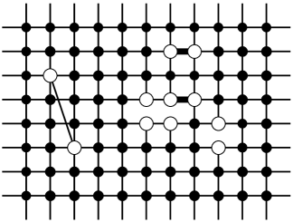
Figure 10.1. A piece of an infinite lattice with some deviations from perfect periodicity. One bar has been added, three bars have been removed, and two bars have been strengthened. The set $\Omega_{\rm inc}$ of effected nodes has 11 elements, which are marked with white circles.

The lattice FMM described in this paper can be used to handle many lattices featuring local deviations from perfect periodicity due to, e.g., missing bars or lattice inclusions, see Figure 10.1. To illustrate, let us consider the equation

(10.1) $$[(\mathsf{A}+\mathsf{B})u](\bm{m})=0,\qquad\bm{m}\in\mathbb{Z}^{2},$$

where $\mathsf{A}$ is the discrete Laplace operator (1.2), and where $\mathsf{B}$ is an operator corresponding to some local modifications to the lattice, such as those illustrated in Figure 10.1. A typical far-field condition of interest is to require that the potential $u$ approaches a linear function, say $v(\bm{m})=c_{1}m_{1}+c_{2}m_{2}$ where $c_{1}$ and $c_{2}$ are given constants, at infinity. Formally, we require

(10.2) $$\lim_{|\bm{m}|\rightarrow\infty}\bigl{|}u(\bm{m})-v(\bm{m})\bigr{|}=0.$$

(In what follows, any function $v$ satisfying $\mathsf{A}v=0$ would work.) When we have access to the solution operator $\mathsf{S}$, defined via

$$[\mathsf{S}u](\bm{m})=\sum_{\bm{n}\in\mathbb{Z}^{2}}\phi(\bm{m}-\bm{n})\,u(\bm{n}),$$

then the equation (10.1), which is a sparse equation defined on the infinite lattice $\mathbb{Z}^{2}$, can be transformed to a dense equation defined only on the set $\Omega_{\rm inc}$ of nodes which connect to bars whose conductivity has been changed, or to which new bars have been connected.

To execute the reduction of (10.1) to an equation defined on $\Omega_{\rm inc}$, set

$$u=v+w,$$

and observe that since $\mathsf{A}v=0$ and $(\mathsf{A}+\mathsf{B})u=0$, the new unknown $w$ must satisfy

(10.3) $$(\mathsf{A}+\mathsf{B})\,w=-\mathsf{B}\,v.$$

Since $\lim_{|\bm{m}|\rightarrow\infty}\bigl{|}w(\bm{m})\bigr{|}=0$, we have $\mathsf{S}\,\mathsf{A}\,w=w$, and so application of $\mathsf{B}\mathsf{S}$ to (10.3) results in the equation

(10.4) $$\mu+\mathsf{B}\,\mathsf{S}\,\mu=-\mathsf{B}\,\mathsf{S}\,\mathsf{B}\,v,$$

where

$$\mu=\mathsf{B}\,w.$$

The key observation is now that $\mathsf{B}$ is a local operator on $\Omega_{\rm inc}$, so equation (10.4) can be restricted to $\Omega_{\rm inc}$ to obtain a closed equation for $\mu$. Once $\mu$ has been solved from this equation, the original potential $u$ is recovered via

$$u=v-\mathsf{S}\,(\mathsf{B}\,v-\mu).$$

It has been demonstrated [10] that iterative solvers in many situations converge rapidly when used to solve a system such as (10.4). The dense coefficient matrix can rapidly be applied to a vector since $\mathsf{B}$ is a sparse operator, and since $\mathsf{S}$ is amenable to the lattice FMM described in this paper.

10.2. Finite lattice problems involving boundary conditions

The lattice FMM described in this paper can also be used in a solution technique for boundary value problems. To illustrate, let us consider the Dirichlet problem

(10.5) $$\left\{\begin{split}[\mathsf{A}\,u](\bm{m})&=0,\hskip 39.83385pt\bm{m}\in\Omega,\\ u(\bm{m})&=g(\bm{m}),\qquad\bm{m}\in\Gamma.\end{split}\right.$$

When we have access to the solution operator $\mathsf{D}$, defined

(10.6) $$[\mathsf{D}u](\bm{m})=\partial_{\bm{n}}\phi(\bm{m}-\bm{n})q(n)$$

where the subscript $\bm{n}$ in $\partial_{\bm{n}}$ simply indicates that the difference operator is acting on the variable $\bm{n}$, then the equation (10.5) can be reduced to a problem defined on $\Gamma$.

An equation for $q$ is obtained by simply restricting (10.6) to $\Gamma$:

(10.7) $$\sum_{n\in\Gamma}d(\bm{m},\bm{n})\,q(\bm{n})=g(\bm{m}),\qquad\bm{m}\in\Gamma.$$

It has been shown in [10] that there exist an $O(N_{\Gamma})$ inversion scheme for solving (10.7). The operator $\mathsf{D}$ can be applied rapidly to $q$ using the lattice FMM described in this paper.

Also in [10], the technique described in this section and in section 10.1 has been put together to create a fast solver for finite lattice problems involving boundary conditions and inclusions. A key tool for the fast solver is the lattice FMM described in this paper.

11. Concluding remarks

The paper presents a kernel independent FMM for solving Poisson problems defined on the integer lattice $\mathbb{Z}^{2}$. For simplicity of presentation, we focused on equations involving the discrete Laplace operator. Techniques for evaluating the corresponding lattice fundamental solutions are presented. The complexity of the proposed method is $O(N_{\rm source})$ where $N_{\rm source}$ is the number of locations in $\mathbb{Z}^{2}$ subjected to body loads.

Numerical experiments demonstrate that for problems where the body loads are sparsely distributed in a computational box the proposed method is faster and more robust than the FFT. For instance, it was demonstrated that using a standard desktop PC, a lattice Poisson equation on a lattice with $N_{\rm domain}=10^{12}$ nodes, of which $N_{\rm source}=10^{6}$ were loaded, was solved to ten digits of accuracy in three minutes. It should be noted that this problem is about six orders of magnitude larger than the largest Poisson problem that can be handled via the FFT. Also, it was demonstrated for a lattice Poisson problem in a domain with $N_{\rm domain}=4,194,304$ nodes, the lattice FMM is faster than the FFT when the number of loaded points is less than $N_{\rm source}=16,384$.

References

- [1] C. R. Anderson, An implementation of the fast multipole method without multipoles, SIAM J. Sci. Statist. Comput. 13 (1992), no. 4, 923–947.
- [2] L. Beatson and L. Greengard, A short course on fast multipole methods.
- [3] William L. Briggs, Van Emden Henson, and Steve F. McCormick, A multigrid tutorial, second ed., Society for Industrial and Applied Mathematics (SIAM), Philadelphia, PA, 2000. MR MR1774296 (2001h:65002)
- [4] Greengard L. Carrier, J. and Rokhlin V., A fast adaptive multipole algorithm for particle simulations, SIAM J. Sci. and Stat. Comput. 9 (1988), no. 4, 669–686.
- [5] H. Cheng, Z. Gimbutas, P. G. Martinsson, and V. Rokhlin, On the compression of low rank matrices, SIAM J. Sci. Comput. 26 (2005), no. 4, 1389–1404 (electronic). MR MR2143489 (2006a:65067)
- [6] V.S. Deshpande, N.A. Fleck, and M.F. Ashby, Effective properties of the octet-truss lattice material, Journal of the Mechanics and Physics of Solids 49 (2001), no. 8, 1747 – 1769.
- [7] R. J. Duffin, Discrete potential theory, Duke Math. J. 20 (1953), 233–251. MR 16,1119d
- [8] R. J. Duffin and E. P. Shelly, Difference equations of polyharmonic type, Duke Math. J. 25 (1958), 209–238.
- [9] M.H. Ernst and P.F.J. Van Velthoven, Random walks on cubic lattices with bond disorder, Journal Journal of Statistical Physics 45 (1986), no. 5-6, 1001–1030.
- [10] A. Gillman and P.G. Martinsson, Fast and accurate numerical methods for solving elliptic difference equations defined on lattices, J. Comput. Phys. 229 (2010), no. 24, 9026–9041.
- [11] Zydrunas Gimbutas and Vladimir Rokhlin, A generalized fast multipole method for nonoscillatory kernels, SIAM J. Sci. Comput. 24 (2002), no. 3, 796–817 (electronic). MR MR1950512 (2004a:65176)
- [12] L. Greengard and V. Rokhlin, A fast algorithm for particle simulations, J. Comput. Phys. 73 (1987), no. 2, 325–348.
- [13] Leslie Greengard, The rapid evaluation of potential fields in particle systems, ACM Distinguished Dissertations, MIT Press, Cambridge, MA, 1988. MR MR936632 (89k:31008)
- [14] Leslie Greengard and Vladimir Rokhlin, A new version of the fast multipole method for the Laplace equation in three dimensions, Acta numerica, 1997, Acta Numer., vol. 6, Cambridge Univ. Press, Cambridge, 1997, pp. 229–269.
- [15] Ming Gu and Stanley C. Eisenstat, Efficient algorithms for computing a strong rank-revealing QR factorization, SIAM J. Sci. Comput. 17 (1996), no. 4, 848–869. MR MR1395351 (97h:65053)
- [16] Hansen A. Herrmann, H. J. and S. Roux, Fracture of disordered, elastic lattices in two dimensions, Phys. Rev. B 39 (1989), no. 1, 637–648.
- [17] J. Makino, Yet another fast multipole method without multipoles—pseudoparticle multipole method, J. Comput. Phys. 151 (1999), no. 2, 910–920.
- [18] A. A. Maradudin, E. W. Montroll, G. H. Weiss, Robert Herman, and H. W. Milnes, Green’s functions for monatomic simple cubic lattices, Acad. Roy. Belg. Cl. Sci. Mém. Coll. in-4 deg. (2) 14 (1960), no. 7, 176. MR 22 #7440
- [19] P.G. Martinsson, Fast multiscale methods for lattice equations, Ph.D. thesis, University of Texas at Austin, Computational and Applied Mathematics, 2002.
- [20] P.G. Martinsson and G.J. Rodin, Asymptotic expansions of lattice green’s functions, Proc. Royal Soc. A 458 (2002), no. 2027, 2609 – 2622.
- [21] P.G. Martinsson and V. Rokhlin, An accelerated kernel independent fast multipole method in one dimension, SIAM Journal of Scientific Computing 29 (2007), no. 3, 1160–11178.
- [22] P.G. Martinsson, V. Rokhlin, and M. Tygert, On interpolation and integration in finite-dimensional spaces of bounded functions, Communications in Applied Mathematics and Computational Science 1 (2006).
- [23] E. Schlangen and E. J. Garboczi, New method for simulating fracture using an elastically uniform random geometry lattice, Int. J. Engng. Sci. 34 (1996), no. 10, 1131–1144.
- [24] J. C. Wallach and L. J. Gibson, Mechanical behavior of a three-dimensional truss material, International Journal of Solids and Structures 38 (2001), no. 40-41, 7181 – 7196.
- [25] Y. Wang and P. Mora, Macroscopic elastic properties of regular lattices, J. Mech. Phys. Solids 56 (2008), no. 12, 2459–3474.
- [26] L. Ying, G. Biros, and D. Zorin, A kernel-independent adaptive fast multipole algorithm in two and three dimensions, J. Comput. Phys. 196 (2004), no. 2, 591–626.