LUNA: An algorithm for generating dynamic planet-moon transits

Abstract

It has been previously shown that moons of extrasolar planets may be detectable with the Kepler Mission, for moon masses above $\sim 0.2$ $M_{\oplus}$ (Kipping et al., 2009c). Transit timing effects have been formerly identified as a potent tool to this end, exploiting the dynamics of the system. In this work, we explore the simulation of transit light curves of a planet plus a single moon including not only the transit timing effects but also the light curve signal of the moon itself. We introduce our new algorithm, LUNA, which produces transit light curves for both bodies, analytically accounting for shadow overlaps, stellar limb darkening and planet-moon dynamical motion. By building the dynamics into the core of LUNA, the routine automatically accounts for transit timing/duration variations and ingress/egress asymmetries for not only the planet, but also the moon.
We then generate some artificial data for two feasibly detectable hypothetical systems of interest: a i) prograde and ii) retrograde Earth-like moon around a habitable-zone Neptune for a M-dwarf system. We fit the hypothetical systems using LUNA and demonstrate the feasibility of detecting these cases with Kepler photometry.

1 Introduction

In recent years, the possibility of detecting the moons of extrasolar planets, so-called “exomoons”, has received increased attention (Sartoretti & Schneider, 1999; Han & Han, 2002; Szabó et al., 2006; Simon et al., 2009; Lewis et al., 2008; Kipping, 2009a, b; Sato & Asada, 2009; Kipping, 2010b). Extrasolar moons may be frequent, temperate abodes for life and a determination of their prevalence would mould our understanding of the abundance of life in the Universe. Although many techniques have been proposed, it is the transit method which seems to offer the greatest potential to detect habitable-zone moons in the near-future (Kipping et al., 2009c).

In general, there are two ways in which a moon can be identified using transits. The first of these is the moon’s own transit light curve (Sartoretti & Schneider, 1999) and the second is the family of techniques known as “transit timing effects”. This includes both transit timing variations (TTV) (Sartoretti & Schneider, 1999) and transit duration variations (TDV). Further, TDV has two different components; one due to velocity variations (TDV-V) (Kipping, 2009a) and one due to transit impact parameter variations (TDV-TIP) (Kipping, 2009b). TTV and TDV-TIP are both due to the position of the planet varying in response to the moon’s presence (positional wobble). In contrast, TDV-V is due to velocity variation of the host planet in response to the moon’s presence (velocity wobble). Combining all of these effects allows for a unique solution (see Kipping 2009b for details) for the moon-to-planet mass ratio and exomoon period (and therefore orbital semi-major axis through Kepler’s Third Law).

To perform the observations, highly precise, continuous photometry is required and the Kepler Mission is thought to be the best instrument currently available to conduct such a search (Kipping et al., 2009c). So far, two searches for exomoons have been conducted using the Kepler photometry, utilizing the transit timing techniques on Kepler-4b through 8b (Kipping & Bakos, 2011a) and TrES-2b (Kipping & Bakos, 2011b). Despite null-results (which was expected as all of these planets are hot-Jupiters), the studies indicate sensitivity into the sub-Earth mass regime, as predicted by Kipping et al. (2009c). The transit timing equations are all built around the premise of a constant planet-star separation and constant planetary velocity during the timescale of the transit. Whilst this is generally a good approximation except for moons on very short periods, there is an obvious desideratum to make the expressions dynamic.

A possible problem with the current technique is that if the moon’s light curve is detectable directly, then not only is this an extra piece of data we are ignoring but also it could fundamentally invalidate many of the transit timing methods. The ideal solution would be to simulate both the planet and moon transit light curves, including limb darkening which is critical for Kepler. In addition, these light curves could be computed with the TTV and TDV effects inherently built into the model in a dynamic way. Not only would this improve upon the static approximations made in the TTV/TDV equations, but it would also bring in TTV/TDV of the moon itself.

Before constructing such an algorithm, one must keep the purpose of such a routine in mind. This algorithm will be used to search for exomoons which will be done by fitting light curves with the new algorithm. Given the large number of free parameters and inevitable intricate inter-parameter dependencies, a Monte Carlo based method seems required. Since such methods are inherently computationally expensive making often millions of calls to the simulation routine, then it is clear that any algorithm we design must be very fast to execute. This essentially excludes methods based upon pixelating the star or other numerical methods. The clear requirement then, is a completely analytic algorithm. The list of requirements are:

• Analytic (absolutely no numerical components)

• Dynamic (inherently accounts for all timing effects)

• Limb darkening incorporated (including non-linear laws)

• All orbital elements accounted for (e.g. eccentricity, longitude of the ascending node, etc)

In summary, such an approach would not only offer many advantages over the previous timing methods, but would also be highly practical for conducting a batch-style search for exomoons in archival data. In this paper, we introduce the fundamental equations needed to construct this algorithm, known as LUNA, and apply it in some hypothetical examples.

In §2, we describe the framework for computing the transit light curves of a planet with a moon and outline the assumptions made. Accompanying details on the model used for the sky-projected motions of the planet and moon can be found in the Appendix (§A). In §3, we provide expressions for the eclipsing area of the moon in front of the star in all 27 possible principal configurations. In §4, example transits light curves are generated and re-fitted for habitable-zone exomoons detectable with Kepler-class photometry. Finally, we discuss comparison to previous methods proposed in the literature and provide concluding remarks in §5.

2 Light Curve Generation

2.1 Converting Time to True Anomaly

To generate a light curve, the relative positions of the star, planet and moon must be calculated at every time stamp in the photometric data set in question. In particular, one requires the sky-projected separation between the planet and star, $S_{P*}$, the moon and the star, $S_{S*}$ and the planet and the moon, $S_{PS}$. We direct the reader to the Appendix (§A) for details on the derivation of the expressions for these terms, where we employ an analytic approximation for the three-body problem which we dub as the nested two-body model (Kipping, 2010b). The coordinate system employed throughout is also defined in the Appendix (§A). It can be shown that these three $S$ terms are a function of $f_{B*}$ and $f_{SB}$ which may be written, in general, as a function of time alone. Note that we define $f_{B*}$ as the true anomaly of the planet-moon barycentre around the star and $f_{SB}$ as the true anomaly of the satellite around the planet-moon barycentre. Therefore, a necessary prerequisite is to convert time stamps to true anomalies. Let us begin with considering the standard practice for a planet by itself.

2.1.1 The Planet-Only Case

The planet-only case is a very familiar one. However, we will cover the conversion of time to true anomaly carefully. Writing out the steps explicity will allow us to identify the necessary procedure for the more complicated planet-moon case we will soon face.

Typically, we have a time series running from an initial time stamp of $t_{1}$ up to $t_{N}$ (where $N$ is the total number of measurements) with the time of transit minimum occurring at $\tau$. Our first task is to convert the time array into an $f$ array. To accomplish this we must define a reference point in time at which the true anomaly is known. Whilst we are free to use any reference point we so desire, a typical choice is the time of transit minimum, $\tau$. In the example above, this choice it will change our array to run from $t_{1}^{\prime}(=t_{1}-\tau$) $\rightarrow$ $t_{N}^{\prime}(=t_{N}-\tau)$ with the transit centred at time $t^{\prime}=0$. The true anomaly at the time of transit minimum can be found by solving d$S$/d$f=0$ for $f$. For even a planet-only case, this is non-trivial and leads to a bi-quartic equation (Kipping, 2008). The solution may be found by a series expansion about the point of inferior conjunction $f(t=\tau)=\pi/2-\omega+\eta$, where $\eta$ represents a perturbation term, which is given up to $6^{\mathrm{th}}$-order in Kipping (2011).

The third and final step is the application of Kepler’s Equation. With the reference true anomaly known, this is converted to a reference mean anomaly via the usual relations (Murray & Dermott, 1999). Then, the mean anomalies at all times may be calculated since this parameter scales linearly with time. Finally, the mean anomalies are converted into true anomalies using Kepler’s Equation.

So to summarize we have three steps: i) subtract the time of transit minimum from all times ii) define the reference anomaly as the time of transit minimum iii) assign mean anomalies for all times, which are then converted to true anomalies using Kepler’s Equation.

For data spanning multiple transits, the reference time should be close to the weighted mean transit number. This selection typically minimizes the correlation between the orbital period and reference time. In such a case, the range of allowed values for the fitting routine to explore vary from $\tau=(\tau_{\mathrm{guess}}-P/2)\rightarrow(\tau_{\mathrm{guess}}+P/2)$. Moving outside of this range would cause the fitting routine to assign a different transit epoch as the reference transit instead.

2.1.2 The Planet-Moon Case

Now consider a planet with a moon. The barycentre of the planet-moon system essentially behaves in the same way which was used to describe the planet-only case. The observed time of transit minimum of the planet is displaced from a linear ephemeris by a small time $\delta t$, due to transit timing variations (Kipping, 2009a). However, the barycentre behaves identically to before and still passes the star at a minimum when $f_{B*}=(\pi/2-\omega_{B*}+\eta)$. Therefore, there is no need to change anything here except that it is understood that the $\tau$ value we fit for is not the time of transit minimum of the planet but the time of transit minimum of the planet-moon barycentre across the star, and thus we denote it as $\tau_{B*}$.

For the moon, an analogous logic may be followed. There must exist a second time shift, $\tau_{SB}$, to account for the phasing between the moon in its orbit around the barycentre. It also seems clear that this phase time has a range of $P_{SB}$ (orbital period of the moon around the barycentre), in analogy to the $\tau_{B*}$ case. Let us imagine we have subtracted $\tau_{B*}$ from all of our times so are left with times running from, say, $t_{1}^{\prime}\rightarrow t_{N}^{\prime}$. The obvious deduction is that we must now subtract a value $\tau_{SB}$ to get to a new time frame $t^{\prime\prime}$, just as we did for $\tau_{B*}$.

A natural choice for $\tau_{SB}$ is the instant when d$S_{SB}$/d$f_{SB}=0$. In analogy to the previous case, this occurs at $f_{SB}=\pi/2-\omega_{SB}+\eta_{SB}$, where $\eta_{SB}$ is the perturbation term. Because this parameter is a phasing term, we prefer to use $\phi_{SB}=(2\pi\tau_{SB})/P_{SB}$ as a definition, to decrease the correlations with the orbital period.

2.2 Retrograde Orbits

A unique problem with LUNA is that exomoons can be either prograde or retrograde. Whilst for planets this is also true, it actually makes no difference to the transit light curve (although the Rossiter-McLaughlin phenomenon is affected). However, for a moon the sense of motion is distinguishable via the TTV and TDV effects (Kipping, 2009b), meaning it does affect the transits and so cannot be neglected.

We tackle this by treating retrograde moons as having $\pi<i_{SB}<2\pi$ and prograde moons as having $0<i_{SB}<\pi$. It is shown in Kipping (2011) that this definition produces the correct retrograde behaviour for the selected coordinate system.

We point out that the asymmetry between prograde and retrograde moons is small. The source of the asymmetry comes from the relative phase difference between the TDV-V and TDV-TIP effects, which is $0$ for prograde moons and $\pi$ for retrograde (Kipping, 2009b). Therefore, the determination of the sense of orbital motion is only generally possible if both TDV-V and TDV-TIP effects are observable.

2.3 Small-Moon Approximation

From a naive perspective, one might start by considering that the transit light curve of a planet and a moon can be computed by calculating the light curve of both separately and then simply adding the signals together. However, there exists numerous scenarios where this would break down. For example, the moon could be eclipsing the star but fully inside the planetary disc and thus the change in flux caused by the moon would be zero.

To overcome this, we start by generating the planetary light curve in the normal way. This can be done using the Mandel & Agol (2002) routine with any limb darkening law we wish and not making any size approximations. Having computed this curve, we need to add on the contribution from the moon. What really matters is what part of the moon is “actively” transiting the star. We define this as the area of the moon which overlaps the star but does not overlap the planet. If we can find this area, then we could compute a light curve for a planet + moon without any limb darkening effects immediately, which is a necessary first step. The subject of the moon’s actively transiting area will be derived later in §3.

For now, let us assume we know what this area is and continue to think about how the limb darkened light curve of the actively transiting moon can be computed. In general, we are interested in achieving two things i) focussing on moons rather than, say, binary-planets ii) actually detecting such signals. The first of these means we are dealing with small objects such that $s\lesssim 0.1$ in all cases and most likely $s\lesssim 0.01$ in most cases (where $s$ is the ratio of the satellite-to-star radii). The second point means that we need to be able to perform fits of transit light curves including all of the planet and moon properties. The inevitably large amount of parameter space necessitates computationally efficient and expedient algorithms. Putting these two arguments together indicates that the best way forward is to employ the small-planet approximation case used in Mandel & Agol (2002). This will ensure accurate modelling of the limb darkening but very fast algorithms.

We stress that the planet is still modelled using the full equations since the host planet could be a Jupiter sized object, yielding $p>0.1$ (where $p$ is the ratio of the planet-to-star radii). Therefore, we assume the moon is small and the planet is not. One limitation of this assumption is “binary-Jupiters”. If we have a binary-planet system for which the smaller body satisfies $s>0.1$ then the algorithm we develop here will be limited in accuracy. However, the current focus of LUNA is solely to detect small bodies.

2.4 Limb Darkened Light Curve for the Actively Transiting Lunar Component

2.4.1 Uniform source

Let us assume that the component of the moon’s area which actively transits the star is known and equals $A_{S,\mathrm{transit}}$. Before we can compute the resulting limb darkened light curve from this component, we must first consider the case for a uniform source.

We start by assuming the actively transiting component of the moon is equal to that which would transit in the absence of a planet. In other words, we here ignore the planet and will re-introduce it later. We follow the methodology of Mandel & Agol (2002), where the ratio of obscured to unobscured flux is given as $F_{S}^{e}(s,S_{S*})=1-\lambda_{S}^{e}(s,S_{S*})$ (replacing the appropriate symbols for the exomoon case):

$$\lambda_{S}^{e}(s,S_{S*})=\left\{\begin{array}[]{ll}0&1+s<S_{S*}\\ \frac{1}{\pi}\left[s^{2}\kappa_{0}+\kappa_{1}-\kappa_{2}\right]&|1-s|<S_{S*}\leq 1+s\\ s^{2}&S_{S*}\leq 1-s\\ 1&S_{S*}\leq s-1,\\ \end{array}\right.$$ (1)

where $\kappa_{1}=\cos^{-1}[(1-s^{2}+S_{S*}^{2})/2S_{S*}]$, $\kappa_{0}=\cos^{-1}[(s^{2}+S_{S*}^{2}-1)/2sS_{S*}]$ and $\kappa_{2}=0.5\sqrt{4S_{S*}^{2}-(1+S_{S*}^{2}-s^{2})^{2}}$.

The most interesting case is clearly $(1-s)\leq S_{S*}\leq(1+s)$, where only a portion of the moon transits the star. The area of the moon which transits the star may be denoted as $\alpha_{S*}$ where the subscript indicates $S$ is transiting $*$.

In this case, $\lambda_{S}^{e}=\alpha_{S*}/\pi$, but $\alpha$ really generally describes the area of intersection between any two circles. We prefer to generalize the equations at this stage, which will prove useful later. Therefore, the area of intersection caused by object of radius $r$ transiting object of radius $R$, with separation $S$, is:

$$\alpha(R,r,S) =r^{2}\kappa_{0}(R,r,S)+R^{2}\kappa_{1}(R,r,S)-\kappa_{2}(R,r,S)$$ (2)

$$\kappa_{0}(R,r,S) =\arccos\Big{[}\frac{S^{2}+r^{2}-R^{2}}{2Sr}\Big{]}$$ (3)

$$\kappa_{1}(R,r,S) =\arccos\Big{[}\frac{S^{2}+R^{2}-r^{2}}{2SR}\Big{]}$$ (4)

$$\kappa_{2}(R,r,S) =\sqrt{\frac{4S^{2}R^{2}-(R^{2}+S^{2}-r^{2})^{2}}{4}}$$ (5)

Let us now re-introduce the planet. The consequences are that in various circumstances the portion of the moon’s shadow which actively transits the star is diminished due to overlap between the planet and the moon. We will discuss the derivation of the actively transiting lunar area in §3, but for now it is sufficient to say that for a uniform source the loss of light due to the lunar component is:

$$F_{S}^{e}(s,S_{S*})=1-\frac{A_{S,\mathrm{transit}}}{\pi}$$ (6)

As an example, in the case of no overlap between the planet and the moon, but the moon fully inside the stellar disc, $A_{S,\mathrm{transit}}=\pi s^{2}$ and thus we recover the expected form shown in Equation 1.

2.4.2 List of Cases

Looking at the equations for a uniform source (Equation 1), one may identify three distinct cases: i) moon fully outside the stellar disc ii) moon partially inside the stellar disc iii) moon fully inside the stellar disc. The first of these is trivial; there is no transit occurring. The third is also trivial for a uniform source but not so for a limb darkened one. For reasons which become clearer later, it is necessary to separate ii) into two different cases dependent upon whether the moon overlaps the stellar centre or not (cases III and IX in the original Mandel & Agol (2002) assignment). To summarize the different cases of interest, we direct the reader to Table 1.

Table 1: List of cases identified by Mandel & Agol (2002). We use the same case notation in this work, but modifying them to emphasise the focus on moons.

Case	Condition	Area of star which is eclipsed
I	$1+s<S_{S*}<\infty$	$0$
II	$1-s<S_{S*}<1+s$	$\alpha_{S*}$
III	$s<S_{S*}<1-s$	$\pi s^{2}$
IX	$0<S_{S*}<s$	$\pi s^{2}$

2.4.3 Case III

Under the assumption of a small ratio-of-radii ($s\ll 1$) one may assume the surface brightness of the star is constant under the disc of the transiting body (Mandel & Agol, 2002). We will here assume non-linear limb darkening of the form $I(r)=1-\sum_{n=1}^{4}c_{n}(1-\mu^{n/2})$, where $I(r)$ represents the radial intensity distribution from the star with $I(0)=1$, $\mu=\cos\theta=\sqrt{1-r^{2}}$ and $r$ is the normalized radial coordinate on the disc of the star. The non-linear limb darkening law (Claret, 2000) is chosen as it may be easily used to compute lower order limb darkening laws, specifically quadratic and linear laws.

Let us draw an annulus inside the star with width $2s$ at radius $S_{S*}$ to represent this surface. We begin by considering case III, where the body is fully inside the star but does not cover the stellar centre (i.e. $s<S_{S*}<1-s$). We have:

$$F_{\mathrm{total}} =\int_{0}^{1}2rI(r)\,\mathrm{d}r$$

$$=1-\sum_{n=1}^{4}\frac{nc_{n}}{n+4}$$ (7)

$$F_{S,\mathrm{annulus}}^{\mathrm{III}}(S_{S*},s) =\int_{S_{S*}-s}^{S_{S*}+s}2rI(r)\,\mathrm{d}r$$

$$=\frac{4}{5}c_{1}\Bigg{[}s^{2}\left(\sqrt[4]{1-b_{m}}-\sqrt[4]{1-a_{m}}\right)$$

$$+\left(S_{S*}^{2}-1\right)\left(\sqrt[4]{1-b_{m}}-\sqrt[4]{1-a_{m}}\right)$$

$$+sS_{S*}\left(2\sqrt[4]{1-a_{m}}+2\sqrt[4]{1-b_{m}}-5\right)\Bigg{]}$$

$$+\frac{2}{21}\Bigg{[}7c_{2}\Big{[}(s^{2}\left(\sqrt{1-b_{m}}-\sqrt{1-a_{m}}\right)$$

$$+\left(S_{S*}^{2}-1\right)\left(\sqrt{1-b_{m}}-\sqrt{1-a_{m}}\right)$$

$$+2sS_{S*}\left(\sqrt{1-a_{m}}+\sqrt{1-b_{m}}-3\right)\Big{]}$$

$$-6\Big{[}c_{3}\Big{(}s^{2}\left(\left(1-a_{m}\right)^{3/4}-(1-b_{m})^{3/4}\right)$$

$$+S_{S*}^{2}\left(\left(1-a_{m}\right)^{3/4}-(1-b_{m})^{3/4}\right)$$

$$+sS_{S*}\left(-2\left(1-a_{m}\right)^{3/4}-2(1-b_{m})^{3/4}+7\right)$$

$$-\left(1-a_{m}\right)^{3/4}+(1-b_{m})^{3/4}\Big{)}$$

$$+7sS_{S*}\left(c_{4}\left(s^{2}+S_{S*}^{2}\right)-1\right)\Big{]}\Bigg{]}$$ (8)

where $a_{m}=(S_{S*}-s)^{2}$ and $b_{m}=(S_{S*}+s)^{2}$ and the $m$ subscript denotes this definition comes from Mandel & Agol (2002). A further simplification is possible by using $a_{mr}=(1-a_{m})^{1/4}$ and $b_{mr}=(1-b_{m})^{1/4}$.

$$F_{S,\mathrm{annulus}}^{\mathrm{III}}(S_{S*},s) =\frac{4}{5}\Big{[}s^{2}(b_{mr}-a_{mr})+(S_{S*}^{2}-1)(b_{mr}-a_{mr})$$

$$+2sS_{S*}\Big{(}-\frac{5}{2}+a_{mr}+b_{mr}\Big{)}\Big{]}c_{1}$$

$$+\frac{2}{21}\Bigg{[}7\Big{(}s^{2}(b_{mr}^{2}-a_{mr}^{2})+(S_{S*}^{2}-1)(b_{mr}^{2}-a_{mr}^{2})$$

$$+2sS_{S*}(-3+a_{mr}^{2}+b_{mr}^{2})\Big{)}c_{2}$$

$$-6\Bigg{(}\Big{(}b_{mr}^{3}-a_{mr}^{3}+2sS_{S*}(\frac{7}{2}-a_{mr}^{3}-b_{mr}^{3})$$

$$+s^{2}(a_{mr}^{3}-b_{mr}^{3})+S_{S*}^{2}(a_{mr}^{3}-b_{mr}^{3})\Big{)}c_{3}$$

$$+7sS_{S*}(-1+(s^{2}+S_{S*}^{2})c_{4})\Bigg{)}\Bigg{]}$$ (9)

The final step is to acknowledge that the transiting body does not transit an area equal to that of the annulus, but in general, a smaller area. Therefore, we must multiply the flux from the annulus by a ratio-of-areas given by:

$$\mathcal{A}_{S}^{\mathrm{III}} =\frac{A_{S,\mathrm{transit}}}{A_{S,\mathrm{annulus}}^{\mathrm{III}}}$$ (10)

$$=\frac{A_{S,\mathrm{transit}}}{\pi[(S_{S*}+s)^{2}-(S_{S*}-s)^{2}]}$$

$$\mathcal{A}_{S}^{\mathrm{III}} =\frac{A_{S,\mathrm{transit}}}{\pi(b_{m}-a_{m})}$$ (11)

The final flux is given by:

$$F_{S}^{e}=1-\mathcal{A}_{S}^{e}\Big{(}\frac{F_{S,\mathrm{annulus}}^{e}}{F_{\mathrm{total}}}\Big{)}$$ (12)

2.4.4 Case IX

If the transiting body has an equatorial orbit, such that $S_{S*}<s$, the setup for case III is invalid since one of the integration limits is negative and $r$ is strictly defined to be $r\geq 0$. This gives us case IX:

$$F_{S,\mathrm{annulus}}^{\mathrm{IX}} =\int_{0}^{S_{S*}+s}2rI(r)\,\mathrm{d}r$$

$$=\frac{4}{5}\Bigg{[}1-b_{mr}+(s+S_{S*})^{2}\Big{(}-\frac{5}{4}+b_{mr}\Big{)}\Bigg{]}c_{1}$$

$$+\frac{2}{3}\Bigg{[}1-b_{mr}^{2}+(s+S_{S*})^{2}\Big{(}-\frac{3}{2}+b_{mr}^{2}\Big{)}\Bigg{]}c_{2}$$

$$+\frac{1}{14}\Bigg{[}14(s+S_{S*})^{2}-7(s+S_{S*})^{4}c_{4}$$

$$+2\Big{(}4-4b_{mr}^{3}+(s+S_{S*})^{2}(-7+4b_{mr}^{3})\Big{)}c_{3}\Bigg{]}$$ (13)

For the ratio of the annulus to actively-transiting-lunar area we have:

$$\mathcal{A}^{\mathrm{IX}} =\frac{A_{S,\mathrm{transit}}}{\pi b_{m}}$$ (14)

2.4.5 Case II

The final case we need is case II. This is when the body is in the ingress/egress portion i.e. $(1-s)<S_{S*}<(1+s)$. In this case the annulus flux is given by:

$$F_{S,\mathrm{annulus}}^{\mathrm{II}} =\int_{S_{S*}-s}^{1}2rI(r)\,\mathrm{d}r$$

$$=\frac{1}{5}(-5+4a_{mr})a_{mr}^{4}c_{1}$$

$$+\frac{a_{m}-1}{42}\Bigg{[}-42+(42-28a_{mr}^{2})c_{2}+6(7-4a_{mr}^{3})c_{3}$$

$$+21(1+a_{m})c_{4}\Bigg{]}$$ (15)

The ratio of the annulus to actively-transiting-lunar area is:

$$\mathcal{A}^{\mathrm{II}} =\frac{A_{S,\mathrm{transit}}}{\pi(1-a_{m})}$$ (16)

2.5 Summary

The light curve of the actively-transiting-lunar component has now been evaluated, but we have not yet derived $A_{S,\mathrm{transit}}$: the sky-projected area of this component. The planetary light curve is computed using the usual Mandel & Agol (2002) routine, utilizing $S_{P*}$. The only remaining task is therefore to find $A_{S,\mathrm{transit}}$, which we deal with next in §3.

3 Actively Transiting Lunar Area

3.1 Principal Cases

The one-body case is described by one parameter, $S$, which can have three states. As we saw in §2, the light curve of the actively-transiting-lunar component can be generated in each case by just knowing $S_{S*}$ and $A_{S,\mathrm{transit}}$, in the small moon approximation. In what follows, we always assume $s^{2}<p^{2}<1$ where $s=R_{S}/R_{*}$. It is therefore clear that our task is to find $A_{S,\mathrm{transit}}$ in all possible configurations i.e. the actively transiting area. This will enable us to compute $\mathcal{A}^{e}$ in cases II, III and IX and thus produce limb darkened transit light curves for the moon.

With three $S$ values now in play ($S_{P*}$, $S_{S*}$ & $S_{SP}$) more cases are possible than before. In total $3^{3}=27$ principal cases exist, but many of these are unphysical under the conditions that $R>p>s$ (where $R=1$) and that $S_{PS}<|S_{P*}-S_{S*}|$. In Table 2, we list all the possible cases by permuting each $S$ parameter into each of their respective three states. The cases which are unphysical are marked accordingly. Figures 1, 2 & 3 illustrate example configurations for each principal case.

Table 2 shows that for some cases, the amount of lunar area actively transiting the star is dependent upon the position of the planet (these case are marked with a *). This is because the planet’s shadow overlaps with the lunar shadow and so the the moon cannot block out to its full potential. We label these cases as exhibiting “areal interaction”.

Table 2: List of principal cases. For each case we label whether the case is geometrically physical or not. We also give the expected eclipsed area due to each body. More complicated cases are marked with a * and exhibit areal interaction. ** indicates multiple sub-cases exist, which is discussed in 3.2.

Case Number [$\mathcal{E}$]	$S_{P}$	$S_{S}$	$S_{PS}$	Physical?	$A_{P,\mathrm{transit}}$	$A_{S,\mathrm{transit}}$
1	$S_{P*}\geq 1+p$	$S_{S*}\geq 1+s$	$S_{PS}\geq p+s$	$\surd$	$0$	$0$
2	$S_{P*}\geq 1+p$	$S_{S*}\geq 1+s$	$p-s<S_{PS}<p+s$	$\surd$	$0$	$0$
3	$S_{P*}\geq 1+p$	$S_{S*}\geq 1+s$	$S_{PS}\leq p-s$	$\surd$	$0$	$0$
4	$S_{P*}\geq 1+p$	$1-s<S_{S*}<1+s$	$S_{PS}\geq p+s$	$\surd$	$0$	$\alpha_{S*}$
5	$S_{P*}\geq 1+p$	$1-s<S_{S*}<1+s$	$p-s<S_{PS}<p+s$	$\surd$	$0$	$\alpha_{S*}$
6	$S_{P*}\geq 1+p$	$1-s<S_{S*}<1+s$	$S_{PS}\leq p-s$	$\times$	-	-
7	$S_{P*}\geq 1+p$	$S_{S*}\leq 1-s$	$S_{PS}\geq p+s$	$\surd$	$0$	$\pi s^{2}$
8	$S_{P*}\geq 1+p$	$S_{S*}\leq 1-s$	$p-s<S_{PS}<p+s$	$\times$	-	-
9	$S_{P*}\geq 1+p$	$S_{S*}\leq 1-s$	$S_{PS}\leq p-s$	$\times$	-	-
10	$1-p<S_{P*}<1+p$	$S_{S*}\geq 1+s$	$S_{PS}\geq p+s$	$\surd$	$\alpha_{P*}$	$0$
11	$1-p<S_{P*}<1+p$	$S_{S*}\geq 1+s$	$p-s<S_{PS}<p+s$	$\surd$	$\alpha_{P*}$	$0$
12	$1-p<S_{P*}<1+p$	$S_{S*}\geq 1+s$	$S_{PS}\leq p-s$	$\surd$	$\alpha_{P*}$	$0$
13	$1-p<S_{P*}<1+p$	$1-s<S_{S*}<1+s$	$S_{PS}\geq p+s$	$\surd$	$\alpha_{P*}$	$\alpha_{S*}$
14**	$1-p<S_{P*}<1+p$	$1-s<S_{S*}<1+s$	$p-s<S_{PS}<p+s$	$\surd$	$\alpha_{P*}$	variable
15	$1-p<S_{P*}<1+p$	$1-s<S_{S*}<1+s$	$S_{PS}\leq p-s$	$\surd$	$\alpha_{P*}$	$0$
16	$1-p<S_{P*}<1+p$	$S_{S*}\leq 1-s$	$S_{PS}\geq p+s$	$\surd$	$\alpha_{P*}$	$\pi s^{2}$
17*	$1-p<S_{P*}<1+p$	$S_{S*}\leq 1-s$	$p-s<S_{PS}<p+s$	$\surd$	$\alpha_{P*}$	$\pi s^{2}-\alpha_{SP}$
18	$1-p<S_{P*}<1+p$	$S_{S*}\leq 1-s$	$S_{PS}\leq p-s$	$\surd$	$\alpha_{P*}$	0
19	$S_{P*}\leq 1-p$	$S_{S*}\geq 1+s$	$S_{PS}\geq p+s$	$\surd$	$\pi p^{2}$	$0$
20	$S_{P*}\leq 1-p$	$S_{S*}\geq 1+s$	$p-s<S_{PS}<p+s$	$\times$	-	-
21	$S_{P*}\leq 1-p$	$S_{S*}\geq 1+s$	$S_{PS}\leq p-s$	$\times$	-	-
22	$S_{P*}\leq 1-p$	$1-s<S_{S*}<1+s$	$S_{PS}\geq p+s$	$\surd$	$\pi p^{2}$	$\alpha_{S*}$
23*	$S_{P*}\leq 1-p$	$1-s<S_{S*}<1+s$	$p-s<S_{PS}<p+s$	$\surd$	$\pi p^{2}$	$\alpha_{S*}-\alpha_{SP}$
24	$S_{P*}\leq 1-p$	$1-s<S_{S*}<1+s$	$S_{PS}\leq p-s$	$\times$	-	-
25	$S_{P*}\leq 1-p$	$S_{S*}\leq 1-s$	$S_{PS}\geq p+s$	$\surd$	$\pi p^{2}$	$\pi s^{2}$
26*	$S_{P*}\leq 1-p$	$S_{S*}\leq 1-s$	$p-s<S_{PS}<p+s$	$\surd$	$\pi p^{2}$	$\pi s^{2}-\alpha_{SP}$
27	$S_{P*}\leq 1-p$	$S_{S*}\leq 1-s$	$S_{PS}\leq p-s$	$\surd$	$\pi p^{2}$	$0$

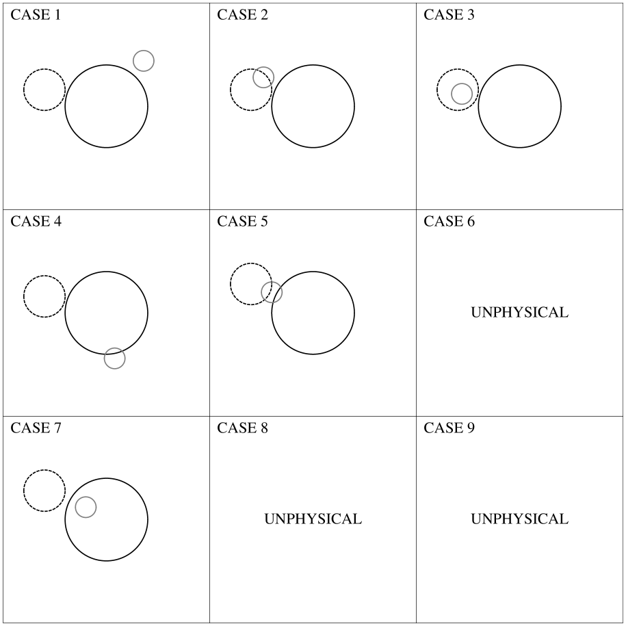
Figure 1: Principal cases 1 to 9. The star is black solid, the planet is black dashed and the moon is gray solid.

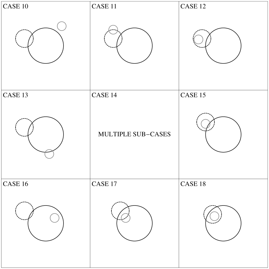
Figure 2: Principal cases 10 to 18. The star is black solid, the planet is black dashed and the moon is gray solid.

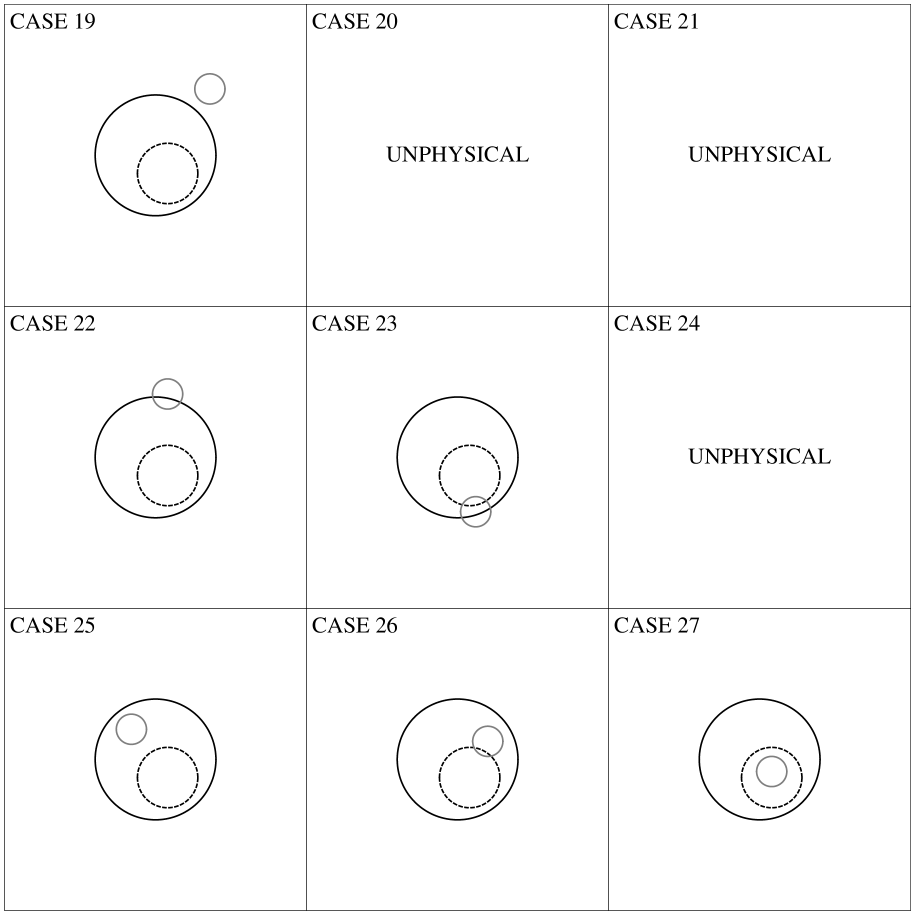
Figure 3: Principal cases 19 to 27. The star is black solid, the planet is black dashed and the moon is gray solid.

3.1.1 Case 26

We start by considering the simplest of the areal interaction cases, case 26 (see Figure 3). We denote this as $\mathcal{E}26$ in mathematical notation (and likewise for the other case numbers). $\mathcal{E}$ is chosen in analogy to the case notation $e$ used by Mandel & Agol (2002). For case 26, the planet and moon are both completely inside the stellar disc but are interacting with each other. This is very similar to the case II situation for a one-body transit where the star has become the planet and the transiting-body has become the moon. So $\{R,p,S\}\rightarrow\{p,s,S_{PS}\}$. The area of the moon which left actively transiting the star is given by $A_{S,\mathrm{transit}}^{\mathcal{E}26}=\pi s^{2}-\alpha_{SP}$.

3.1.2 Case 17

The next most complicated case is case 17. Here the planet is on the limb of the star and the moon is on the limb of the planet, but completely within the star. It can be seen that $A_{S,\mathrm{transit}}^{\mathcal{E}27}=A_{S,\mathrm{transit}}^{\mathcal{E}26}=\pi s^{2}-\alpha_{SP}$ and thus we already have the required equation in hand.

3.1.3 Case 23

The third most complicated case is when the planet is completely inside the star but the moon sits on the planetary limb and coincidentally the stellar limb. If the planet was not present, the moon would eclipse an area given by $\alpha_{S*}$.

However, the planet is present, and it blocks out a portion of this area. Under the conditions of case 23, the overlapping area between the planet and moon must always lie completely within the stellar disc since the planet always lies completely within the stellar disc. It can be therefore be seen that the overlapping area, $\alpha_{SP}$, will always be less than $\alpha_{S*}$. Therefore, the final area which is actively transiting the star from the moon alone is:

$$A_{S,\mathrm{transit}}^{\mathcal{E}23} =\alpha_{S*}-\alpha_{SP}$$ (17)

3.2 The Sub-Cases of Case 14

Case 14 is the most complicated case to consider. Indeed, case 14 actually has multiple sub-cases which define the various possible behaviours. Although similar to case 23, the planet’s shadow now does not completely eclipse the star and so the overlapping area between the moon and planet also does not necessarily have to lie completely within the stellar disc. As a consequence, multiple different states exist and a singular expression is not possible for $A_{S,\mathrm{transit}}$.

The first key question is: how many sub-cases actually exist? The problem we are thinking of is that of three circles interacting to give an overlapping region, for which we require the associated area. The problem of finding the area of overlap between three circles was studied extensively in the pioneering work of Fewell (2006). Indeed, an analytic solution for the overlap of three circles did not exist until 2006 when Fewell presented the solution. Fewell (2006) identified nine possible cases in total, which we label as Fewell case (1) $\rightarrow$ (9) and viewable in Figure 5 of Fewell (2006). To assign identities in our framework, we label the biggest circle the star, the middle-sized circle the planet and the smallest circle the moon in Figure 5 of Fewell (2006).

Going through the Fewell (2006) scenarios with our assigned identities, the first thing we notice is that only four of the Fewell (2006) cases remain consistent with the case 14 conditions, the others are much simpler scenarios which we dealt with earlier as the principal cases. In Table 3, we show the corresponding case numbers to the Fewell (2006) cases for completion.

Table 3: List of Fewell (2006) cases and the corresponding case definitions used in this work.

Fewell (2006) Case Number	Case Number (This work) [$\mathcal{E}$]
(1)	14.1
(2)	14.2
(3)	14.3
(4)	17
(5)	18
(6)	27
(7)	14.7
(8)	11
(9)	10

The Fewell (2006) solution for the area of common overlap between three circles is based upon a formula for the circular triangle, which uses the chord lengths and radii of the three circles involved. Only in Fewell case (1) does a circular triangle actually exist and this is the focus of Fewell (2006). However, Fewell (2006) performs the derivation by calculating analytic expressions for the vertices of all three circles which may then be converted to chord lengths and these equations are useful for distinguishing between all the various sub-cases.

Let us consider three circles labelled 1, 2 and 3 of radii $\mathcal{R}_{i}$ and positions $\{\mathcal{X}_{i},\mathcal{Y}_{i}\}$ and intersection points $\{\mathcal{X}_{ij},\mathcal{Y}_{ij}\}$ (where two intersections points always exist for each $i$-$j$ pairing under the case 14 conditions). Let us define $\{\mathcal{X}_{1},\mathcal{Y}_{1}\}=\{0,0\}$ and assume $\mathcal{R}_{1}>\mathcal{R}_{2}>\mathcal{R}_{3}$. Therefore, we have circle 1 being the star, circle 2 being the planet and circle 3 being the moon. The intersection points are given by (see Fewell (2006) for details of the relevant derivation):

$$\mathbf{Intersection\,\,12}$$

$$\mathcal{X}_{12} =\frac{1-p^{2}+S_{P*}^{2}}{2S_{P*}}$$ (18)

$$\mathcal{Y}_{12} =\frac{1}{2S_{P*}}\sqrt{2S_{P*}^{2}(1+p^{2})-(1-p^{2})^{2}-S_{P*}^{4}}$$ (19)

$$\mathbf{Intersection\,\,13}$$

$$\mathcal{X}_{13} =\mathcal{X}_{13}^{\prime}\cos\theta^{\prime}-\mathcal{Y}_{13}^{\prime}\sin\theta^{\prime}$$ (20)

$$\mathcal{Y}_{13} =\mathcal{X}_{13}^{\prime}\sin\theta^{\prime}+\mathcal{Y}_{13}^{\prime}\cos\theta^{\prime}$$ (21)

$$\mathcal{X}_{13}^{\prime} =\frac{1-s^{2}+S_{S*}^{2}}{2S_{S*}}$$ (22)

$$\mathcal{Y}_{13}^{\prime} =\frac{-1}{2S_{S*}}\sqrt{2S_{S*}^{2}(1+s^{2})-(1-s^{2})^{2}-S_{S*}^{4}}$$ (23)

$$\cos\theta^{\prime} =\frac{S_{P*}^{2}+S_{S*}^{2}-S_{PS}^{2}}{2S_{P*}S_{S*}}$$ (24)

$$\sin\theta^{\prime} =\sqrt{1-\cos^{2}\theta^{\prime}}$$ (25)

$$\mathbf{Intersection\,\,23}$$

$$\mathcal{X}_{23} =\mathcal{X}_{23}^{\prime\prime}\cos\theta^{\prime\prime}-\mathcal{Y}_{23}^{\prime\prime}\sin\theta^{\prime\prime}+S_{P*}$$ (26)

$$\mathcal{Y}_{23} =\mathcal{X}_{23}^{\prime\prime}\sin\theta^{\prime\prime}+\mathcal{Y}_{23}^{\prime\prime}\cos\theta^{\prime\prime}$$ (27)

$$\mathcal{X}_{23}^{\prime\prime} =\frac{p^{2}-s^{2}+S_{PS}^{2}}{2S_{PS}}$$ (28)

$$\mathcal{Y}_{23}^{\prime\prime} =\frac{1}{2S_{PS}}\sqrt{2S_{PS}^{2}(p^{2}+s^{2})-(p^{2}-s^{2})^{2}-S_{PS}^{4}}$$ (29)

$$\cos\theta^{\prime\prime} =-\frac{S_{P*}^{2}+S_{PS}^{2}-S_{S*}^{2}}{2S_{P*}S_{PS}}$$ (30)

$$\sin\theta^{\prime\prime} =\sqrt{1-\cos^{2}\theta^{\prime\prime}}$$ (31)

3.2.1 Fewell Case (1)

What makes Fewell case (1) unique mathematically speaking? i.e. under what conditions are the equations for (1) valid? Fewell (2006) provides expressions for evaluating whether case (1) is satisfied or not. Fewell (2006) identifies “two” conditions but one of these conditions is just the case 14 conditions and need not be considered again. The second condition is actually composed of two causal factors and so in total there exists two conditions which uniquely define case 14.1. Let us define conditions A and B as:

$$\mathbf{Condition\,\,A}$$

$$(\mathcal{X}_{12}-S_{S*}\cos\theta^{\prime})^{2}+(\mathcal{Y}_{12}-S_{S*}\sin\theta^{\prime})^{2}<s^{2}$$ (32)

$$\mathbf{Condition\,\,B}$$

$$(\mathcal{X}_{12}-S_{S*}\cos\theta^{\prime})^{2}+(\mathcal{Y}_{12}+S_{S*}\sin\theta^{\prime})^{2}<s^{2}$$ (33)

In order to have case 14.1, we require that condition A is satisfied and condition B is anti-satisfied (we call this condition $\bar{B}$). The area $\alpha_{\mathrm{transit}}$ may be found by evaluating the circular triangle, principally defined by the chord lengths and radii. In fact, two sub-sub-cases exist here for 14.1 which we label as 14.1a and 14.1b. 14.1a is the case where less than half the circle is involved and 14.1b occurs when more than half the circle is involved. The two cases are distinguished by evaluating the following:

$$\mathbf{Condition\,\,C}$$

$$S_{S*}\sin\theta^{\prime}>\mathcal{Y}_{13}+\frac{\mathcal{Y}_{23}-\mathcal{Y}_{13}}{\mathcal{X}_{23}-\mathcal{X}_{13}}(S_{S*}\cos\theta^{\prime}-\mathcal{X}_{13})$$ (34)

If the above equation is true (condition C) then we have case 14.1a and $A_{\mathrm{overlap}}^{\mathcal{E}14.1a}$ may be found using:

$$A_{\mathrm{overlap}}^{\mathcal{E}14.1a} =\frac{1}{4}\sqrt{(\mathfrak{c}_{1}+\mathfrak{c}_{2}+\mathfrak{c}_{3})(\mathfrak{c}_{2}+\mathfrak{c}_{3}-\mathfrak{c}_{1})}$$

$$\times\sqrt{(\mathfrak{c}_{1}+\mathfrak{c}_{3}-\mathfrak{c}_{2})(\mathfrak{c}_{1}+\mathfrak{c}_{2}-\mathfrak{c}_{3})}$$

$$+\sum_{k=1}^{3}\Big{(}\mathcal{R}_{k}^{2}\arcsin\frac{\mathfrak{c}_{k}}{2\mathcal{R}_{k}}-\frac{\mathfrak{c}_{k}}{4}\sqrt{4\mathcal{R}_{k}^{2}-\mathfrak{c}_{k}^{2}}\Big{)}$$ (35)

$$\mathfrak{c}_{k}^{2} =(\mathcal{X}_{ik}-\mathcal{X}_{jk})^{2}+(\mathcal{Y}_{ik}-\mathcal{Y}_{jk})^{2}$$ (36)

Otherwise (condition $\bar{C}$), for case 14.1b, we must use:

$$A_{\mathrm{overlap}}^{\mathcal{E}14.1b} =\frac{1}{4}\sqrt{(\mathfrak{c}_{1}+\mathfrak{c}_{2}+\mathfrak{c}_{3})(\mathfrak{c}_{2}+\mathfrak{c}_{3}-\mathfrak{c}_{1})}$$

$$\times\sqrt{(\mathfrak{c}_{1}+\mathfrak{c}_{3}-\mathfrak{c}_{2})(\mathfrak{c}_{1}+\mathfrak{c}_{2}-\mathfrak{c}_{3})}$$

$$+\sum_{k=1}^{3}\Big{(}\mathcal{R}_{k}^{2}\arcsin\frac{\mathfrak{c}_{k}}{2\mathcal{R}_{k}}\Big{)}$$

$$-\frac{\mathfrak{c}_{1}}{4}\sqrt{4\mathcal{R}_{1}^{2}-\mathfrak{c}_{1}^{2}}-\frac{\mathfrak{c}_{2}}{4}\sqrt{4\mathcal{R}_{2}^{2}-\mathfrak{c}_{2}^{2}}+\frac{\mathfrak{c}_{3}}{4}\sqrt{4\mathcal{R}_{3}^{2}-\mathfrak{c}_{3}^{2}}$$ (37)

The actively transiting area of the moon is now given by: $A_{S,\mathrm{transit}}^{\mathcal{E}14.1x}=\alpha_{S*}-A_{\mathrm{overlap}}^{\mathcal{E}14.1x}$. In the above equations, it should be noted that $\mathfrak{c}_{k}$ represents the chord lengths.

3.2.2 Fewell Case (2)

Fewell (2006) does not discuss in any detail how to compute the area of overlap for Fewell case (2), but this is simpler than Fewell case (1). In Fewell case (1) we had a circular triangle, whereas case (2) presents a circular quadrilateral. Before we consider the various scenarios, let us define under what conditions Fewell case (2) is satisfied.

For Fewell case (2), the constraint is that the two intersection points of circles 1 and 2 both lie outside of circle 3 (this narrows it down to Fewell case (2) or (7)). Therefore we must satisfy conditions $\bar{A}$ and $\bar{B}$.

Next, the intersection points of circles 1 and 3 must lie inside circle 2 (this distinguishes it from Fewell case (7)). Assuming case 14, condition $\bar{A}$ and condition $\bar{B}$, it is not physically possible to have a solution where one of these intersection points lies inside and the other outside of circle 2. It is, however, possible to have both outside, which gives rise to Fewell case (7). Because of this fact, we only need to use one of the intersection points to define condition D:

$$\mathbf{Condition\,\,D}$$

$$(\mathcal{X}_{13}-S_{P*})^{2}+\mathcal{Y}_{13}^{2}<p^{2}$$ (38)

But, even this is not enough for a unique solution. In Fewell case (2) of Figure 5 of Fewell (2006), one could imagine mirroring the moon along the line connecting the two moon-star intersection points. This would still satisfy all of the above conditions but now no part of the moon is actively transiting. The nominal case, as shown in Figure 5 of Fewell (2006), is labelled as 14.2a (shown in Figure 4), whereas the alternative case is 14.2b. Therefore, we define condition E, which if satisfied gives case 14.2a and if anti-satisfied gives case 14.2b:

$$\mathbf{Condition\,\,E}$$

$$(S_{S*}-s)<(S_{P*}-p)$$ (39)

Case 14.2a has $A_{S,\mathrm{transit}}^{\mathcal{E}14.2a}=\pi s^{2}-\alpha_{SP}$, otherwise for 14.2b we have $A_{S,\mathrm{transit}}^{\mathcal{E}14.2b}=0$.

3.2.3 Fewell Case (3)

To meet Fewell case (3), both intersection points of 1 and 2 must lie inside circle 3 i.e. condition A and B. Sub-case 14.3 contains two possible sub-sub-cases; 14.3a and 14.3b. The second sub-sub-case was identified quite late in our analysis and noticed during testing and debugging.

The two cases are differentiated by whether the planet’s centre is inside or outside the stellar disc. If outside, then we have case 14.3a, which satisifes condition F.

$$\mathbf{Condition\,\,F}$$

$$S_{P*}>1$$ (40)

In this case, 14.3a, $A_{\mathrm{S,transit}}^{\mathcal{E}14.3a}=\alpha_{S*}-\alpha_{P*}$. For case 14.3b, the planet is inside and we have $A_{\mathrm{S,transit}}^{\mathcal{E}14.3b}=\pi p^{2}-\alpha_{SP}-\alpha_{P*}+\alpha_{S*}$.

3.2.4 Fewell Case (7)

For Fewell case (7), we must satisfy conditions $\bar{A}$ and $\bar{B}$, as did Fewell case (2). The final condition for Fewell case (7) is simply the opposite of condition D, i.e. condition $\bar{D}$.

However, this is insufficient to give a unique solution. The standard Fewell case (7) has no interaction between the planet and moon within the stellar disc but this is not a condition, merely an artifact of the figure’s construction. It is possible that the intersection points of 1 and 2 lies outside circle 3, and the intersection points of 1 and 3 lies outside 2, but still two distinct cases exist. These two sub-sub-cases are that if the intersection of 2 and 3 lies within 1, then areal interactions must be occurring. We label this case 14.7b. Case 14.7a is that the circles do not interact.

This first case occurs when both intersection points of 2 and 3 lie outside of circle 1. It is not possible to have one inside and one outside under the previous conditions so far met. Thus we have condition G, which if satisfied yields case 14.7b and if anti-satisfied gives 14.7a.

$$\mathbf{Condition\,\,G}$$

$$\mathcal{X}_{23}^{2}+\mathcal{Y}_{23}^{2}<1$$ (41)

Accordingly, $A_{\mathrm{S,transit}}^{\mathcal{E}14.7a}=\alpha_{S*}$. Otherwise the planet-moon intersections occur within the star and thereby necessitating a degree of interaction (case 14.7b, satisfying condition G), for which $A_{\mathrm{S,transit}}^{\mathcal{E}14.7b}=\alpha_{S*}-\alpha_{SP}$.

3.2.5 Summary of Sub-Cases

This completes every possible scenario for three circles interacting. The sub-case conditions are summarized in Table 4 and illustrated example configurations are shown in Figure 4. We have calculated the area of overlap in every case in an analytic manner. This will allow for extremely expedient computation of the light curve from a planet plus moon.

Due to the plethora of cases, sub-cases and even sub-sub-cases, a large amount of testing of the LUNA algorithm has been executed. This was done by trying various system configurations and ensuring no gaps existed in the case conditions or unusual light curve features were produced by the algorithm. It was during this stage which we identified that sub-case 14.3 actually had two sub-sub-cases in the form of 14.3a and 14.3b.

Table 4: List of sub-cases and conditions. A bar indicates the condition is anti-satisfied.

Sub-Case	Conditions Satisfied	$A_{\mathrm{S,transit}}$
14.1a	A; $\bar{B}$; C	$\alpha_{S*}-A_{\mathrm{overlap}}^{\mathcal{E}14.1a}$
14.1b	A; $\bar{B}$; $\bar{C}$	$\alpha_{S*}-A_{\mathrm{overlap}}^{\mathcal{E}14.1b}$
14.2a	$\bar{A}$; $\bar{B}$; D; E	$\pi s^{2}-\alpha_{SP}$
14.2b	$\bar{A}$; $\bar{B}$; D; $\bar{E}$	0
14.3a	A; B; F	$\alpha_{S*}-\alpha_{P*}$
14.3b	A; B; $\bar{F}$	$\pi p^{2}-\alpha_{P*}-\alpha_{SP}+\alpha_{S*}$
14.7a	$\bar{A}$; $\bar{B}$; $\bar{D}$; $\bar{G}$	$\alpha_{S*}$
14.7b	$\bar{A}$; $\bar{B}$; $\bar{D}$; G	$\alpha_{S*}-\alpha_{SP}$

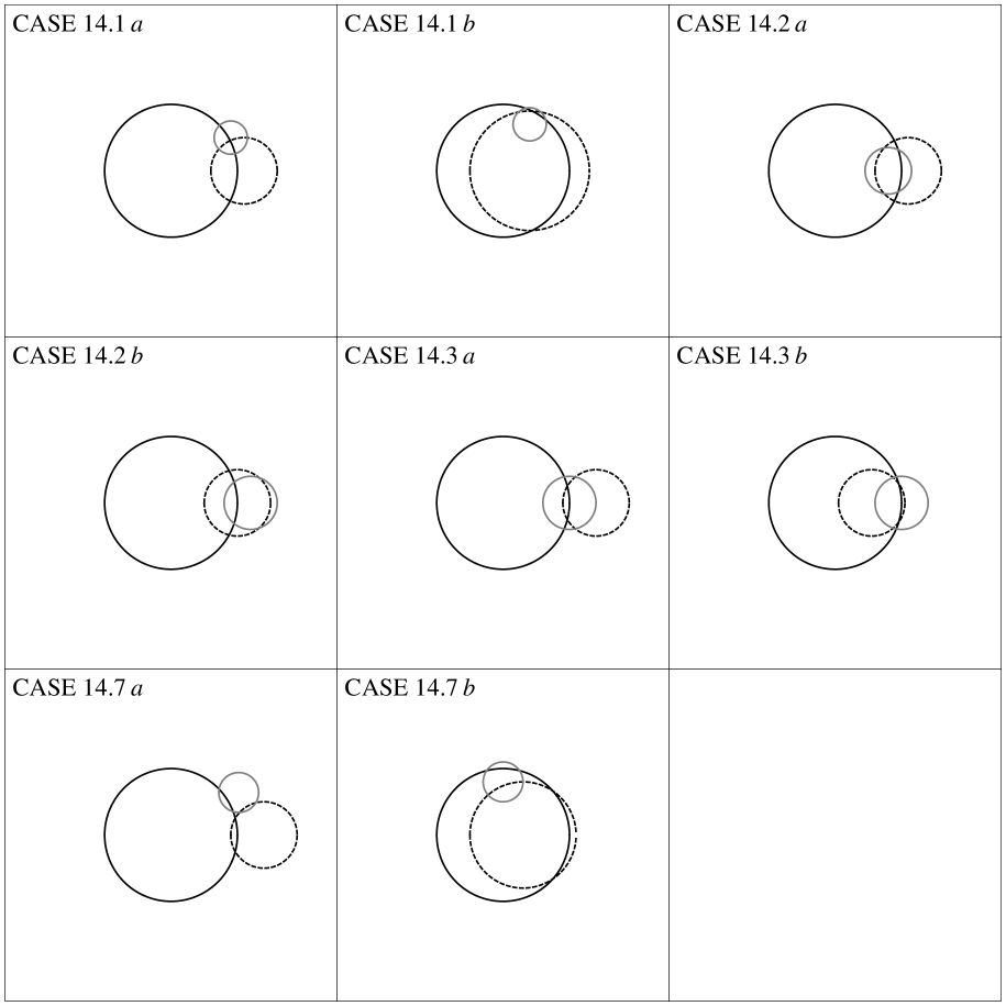
Figure 4: Sub-cases of case 14. The subscript numbers (1,2,3,7) originate from the system employed by Fewell (2006). The extra case conditions (a,b) come from additional complexity within each sub-case yet consistent within the original case definitions of Fewell (2006). The star is black solid, the planet is black dashed and the moon is gray solid. Relative sizes selected purely for depiction purposes.

3.3 Flow Decision Diagram

With all the conditions stated, it is useful to construct a flow diagram of the decision route which LUNA should take. This flow diagram should be designed to minimize the number of calculations LUNA has to perform. We have conditions A to G for the sub-cases and three additional conditions from the principal cases, so the maximum number of decisions in any chain should be 10. Ideally, most decision routes will involve fewer than 10 decisions.

3.3.1 Decision 1

The best-place to start is with the principal cases. The computation of the transit light curve will always require a computation of $S_{P*}$, as it is assumed that the planet always transits.

Since we always have to compute this term anyway, the economic way to proceed is to base a decision tree upon its behaviour. This essentially gives us a three way-split into three decision trees: cases 1 through 9 (called “p-out”), 10 through 19 (“p-part”) and 20 through 27 (“p-in”).

3.3.2 Decision 2

Having computed $S_{P*}$, should we compute $S_{S*}$ and $S_{PS}$? In several cases, only one of these is required to calculate the light curve. Consider, the p-out tree first (note that the second decision does not have to be the same in each tree). Since the planet is out of the stellar disc, areal interaction is impossible and thus $S_{PS}$ need never be computed. Therefore, the logical second decision for p-out is simply to evaluate $S_{S*}$ and see which of the three possible circumstances it is in.

For the p-in tree, there are two possible questions one could pose. Remember, we wish to pose the question which leads to the most efficient algorithm. First possible question: evaluate $S_{S*}$ and see which state it is in. Second possible question: evaluate $S_{SP}$ and see which state it is in.

If we ask the second question, the in-case requires no further computations. However, the part and out cases both require that we evaluate $S_{S*}$ to proceed.

If we ask the first question, the out case requires no further computation. However, the in and part cases require we calculate $S_{SP}$. Therefore, the two approaches seem to yield equivalent levels of complexity. In general, if the moon is transiting, $S_{S*}$ will always be needed whereas $S_{SP}$ is only needed if areal interaction occurs. Therefore, we prefer to ask about $S_{S*}$ first.

Finally, for the p-part tree, case 14 is the mix which is by the far the most complicated case computationally. We wish to choose a tree based upon minimizing our exposure to case 14. $S_{S*}$ again makes a natural choice by the groupings of the actively transiting area formulas.

3.3.3 Decision 3

Since decision 2 is always the same, decision 3 is simply to evaluate $S_{SP}$ and check its condition. There is no choice in this.

3.3.4 Decision 14.1

If case 14 occurs, we have a new decision tree opening up due to presence of sub-cases. The first decision is decision 14.1. Unlike the principal tree, each sub-case does not necessarily involve a calculation of all the possible conditions. Therefore, some conditions crop up more frequently than others. If all the conditions took the same time to compute, then we would prefer to compute those conditions which occur most frequently early on in our decision tree.

Conditions A and B clearly provide the backbone to the decision tree and thus must be evaluated early on. Their evaluation is ultimately unavoidable so should be done at the start. Case 14.3 is unusual in that it can be identified as satisfying condition B only since all sub-cases anti-satisfy B. Condition B is therefore the obvious starting point in our decision tree. If verified, we have case 14.3 and if not we move into decision 14.2.

3.3.5 Decision 14.2

Since conditions A and B are the backbone and B has been evaluated, the next step is to evaluate A. If satisfied, we have case 14.1. Anti-satisfaction means we have either 14.2 or 14.7.

3.3.6 Decision 14.3

If we have 14.1, then decision 14.3 must be to evaluate condition C. If we have 14.2 or 14.7, then the discriminator is condition D.

3.3.7 Decision 14.4

Not needed for 14.1 cases, but for Fewell cases (2) and (7) we must compute conditions E and G respectively.

3.3.8 Summary of decision tree

Figure 5 shows the decision process in a flow chart to summarize the approach of LUNA.

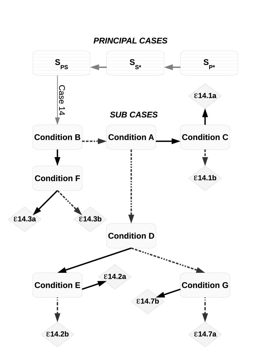
Figure 5: Flow chart showing the decision process of choosing which case we are in. The decision tree has been optimized to marginalize the more CPU intensive computations until absolutely required. The principal cases are not shown but are easily seen in Table 2. Square boxes indicate an evaluation of whatever is inside the box. Black arrows indicate a true statement and the dot-dashed gray arrows indicate a false.

4 Example Transit Light Curves

4.1 Dealing with Inclination

Transit modellers will be familiar with the pot-holes in the road presented when trying to fit transit light curves with the physical parameters. To start with, inclination is almost always in the range $\sim$85 to 90 degrees and fitting for $i_{B*}$ yields large correlations and lethargic routines. In practice, it is better to define the impact parameter of the transit chord across the star, $b_{B*}$.

$$b_{B*}=(r_{B*}/R_{*})\cos i_{B*}$$ (42)

A similar strategy would seem advisable for moons and we can define an analogous quantity:

$$b_{SB}=(r_{SB}/R_{P})\cos i_{SB}$$ (43)

It should be noted that $b_{SB}$ is only the impact parameter in the reference frame of the moving barycentre and will not be the observed impact parameter in the sky frame. Therefore, $b_{SB}$ can be greater than unity and yet the moon still transits the star.

Another subtlety is that $i_{SB}=\pi/2+\delta$ would give a different light curve than $i_{SB}=\pi/2-\delta$, but both would yield the same value for $b_{SB}$ (in contrast to the situation for a planet by itself). To account for this asymmetry, negative impact parameters are perceived as yielding $i_{SB}=\pi-\cos^{-1}[R_{P}b_{SB}/r_{SB}]$. Retrograde satellites with inclinations in the range $\pi<i_{SB}<2\pi$ are adjusted in a second step where if a logical flag for retrograde orbits is switched on, $\pi$ is added onto the inclination.

4.2 Fitting Parameter Set

A typical planetary parameter set would be $\{\tau,p^{2},(a/R_{*}),b\}$. Due the strong correlation between $(a/R_{*})$ and $b$ (Carter et al., 2008), it is preferable to switch one of these parameters for a less correlated term. A typical choice is $\tilde{T}$, the duration for the planet to move from its centre overlapping the stellar limb to exiting under the same condition. An inverse-mapping expression to go from $\tilde{T}$ to $(a/R_{*})$ is given in Kipping (2010a). Note that a $\tilde{T}$ equation for the moon is not possible since $b_{SB}>1$ is permitted and thus $\tilde{T}$ would be complex.

We now have the four fitted parameters $\{\tau_{B*},p^{2},\tilde{T}_{B*},b_{B*}\}$ for the planet-moon barycentre. Additionally, we need the orbital period, $P_{B*}$, which may be fitted for if multiple transits exist. Radial velocity or secondary eclipse information may be used to expand the parameter set to include $e_{B*}\cos\omega_{B*}$ and $e_{B*}\sin\omega_{B*}$. Finally, the out-of-transit flux, OOT, and the blending factor, $B$ (which cannot be fitted for) should also be included. The quadratic limb darkening coefficients $u_{1}$ and $u_{2}$ give an additional two parameters bringing the total to 11. RV data may also require additional terms such as semi-amplitude, $K$, velocity offset, $\gamma$, etc.

To include the exomoon, 9 new parameters are needed: $\{\phi_{SB}$, $(M_{S}/M_{P})$, $s$, $(a_{SB}/R_{*})$, $b_{SB}$, $P_{SB}$, $e_{SB}\cos\omega_{SB}$, $e_{SB}\sin\omega_{SB}$, $\Omega_{SB}\}$. In total, this means we have 20+RV parameters. In practice, not all of these will be fitted for e.g. the blending factor.

4.3 Example Simulations & Fits

In the next three subsections (§4.4-4.6) we provide three simulations generated by LUNA. The system configuration used in each case is discussed in the relevant subsections. In each case, we use a cadence of 1 minute and add on Gaussian noise of 250 ppm, in-line with the properties of Kepler’s short-cadence photometry (Kipping & Bakos, 2011b). Data are produced surrounding $\pm 0.5$ days of $\tau_{B*}$ for $N$ consecutive transit epochs.

These noised light curves are then fitted using a Metropolis-Hastings MCMC routine with 125,000 steps and a 20% burn-in to give $10^{5}$ final points for building the parameter posteriors. Jump-sizes are set to be equal to the 1-$\sigma$ uncertainties (determined through preliminary runs) and the final parameter values are given by the median of each parameter with uncertainties of 34.15% quantiles either side.

For each case, we perform three fits with fixed assumptions i) no moon is present i.e. $s=0$ and $M_{S}/M_{P}=0$ ii) the moon is prograde (i.e. $i_{SB}$ is bounded to be in the range $0<i_{SB}\leq\pi$) iii) the moon is retrograde ($\pi<i_{SB}\leq 2\pi$). In reality, only one case is genuine and the two other act to show how distinguishable each scenario really is. We always assume a circular orbit for the moon and planet for simplicity, which removes four parameters.

In all cases, we utilize a powerful trick pointed out in Kipping (2010b). The detection of a planet-moon system allows one to determine the absolute mass and radius of the host star through Kepler’s Third Law alone. Armed with these parameters, the planetary and lunar physical dimensions may also be obtained, thus replacing the traditional need for invoking spectroscopy and stellar evolution models. The only additional information one requires is the radial velocity semi-amplitude induced by the planet-moon barycentre, $K$. As the observational uncertainty on this parameter scales with $\sim 1/\sqrt{N_{\mathrm{RV}}}$, where $N_{\mathrm{RV}}$ is the number of RV measurements, it can be determined to high precision by simply repeating the radial velocity observations.

As shown in Kipping (2010b), the absolute dimensions of the star have scalings $M_{*}\sim K_{*}^{3}$ and $R_{*}\sim K_{*}$, and so $[\sigma(M_{*})]^{2}\simeq[3\sigma(K_{*})]^{2}+[\sigma(M_{*}^{\prime})]^{2}$ and $[\sigma(R_{*})]^{2}\simeq[\sigma(K_{*})]^{2}+[\sigma(R_{*}^{\prime})]^{2}$, where the dashed terms denote the value derived assuming no error on $K_{*}$. In an example shown later (see §4.5), $K_{*}=6$ m/s and $\sigma(M_{*}^{\prime})/M_{*}^{\prime}\simeq 15\%$ and $\sigma(R_{*}^{\prime})/R_{*}^{\prime}\simeq 6\%$. This example is a singular case but nonetheless serves the purpose of illustrating a feasible situation. In this example, the assumption that $K_{*}$ contributes negligible error into the stellar mass determination is valid for $\sigma(K_{*})/K_{*}\lesssim$2.5% ($\sim 0.15$ m/s) and for the stellar radius $\sigma(K_{*})/K_{*}\lesssim$7.0% ($\sim 0.4$ m/s). These RV precisions are comparable to values being reported by those using high-precision facilities such as Keck and HARPS (Vogt et al., 2010; Lovis et al., 2011). More generally, once an exomoon system is found, the uniqueness and importance of the system would certainly warrant the exploitation of such spectrographic resources and so high levels of precision in $K_{*}$ can be expected.

We therefore assume that the uncertainty on $K_{*}$ is much less than the uncertainty on the photometrically determined exomoon parameters in what follows. The inclusion of the determination of $M_{*}$ and $R_{*}$ using the Kipping (2010b) method will demonstrate the feasibility of the technique.

We note that $s$ and $M_{S}/M_{P}$ are positive definite and thus always yield a non-zero result. To identify cases where this bias is creating a false-positive, we apply the Lucy & Sweeney (1971) test. If $s$ or $M_{S}/M_{P}$ yield a false-alarm-probability below 5%, then we quote the MCMC result as usual. Otherwise, we quote the 95% confidence upper limit on those parameters.

4.4 HZ-Neptune with a Close, Prograde Moon around an M2 Star

4.4.1 Simulation and Fitting

As a first example, we consider a Neptune-mass and radius planet in orbit an M2 star in the habitable-zone ($K_{*}=6.0$ m s^-1). Using the stellar parameters from Cox (2000), we assign $M_{*}=0.40$ $M_{\odot}$ and $R_{*}=0.50$ $R_{\odot}$. We place the planet in an orbital period of $P_{B*}=46.0$ days in a circular orbit with $i_{B*}=90^{\circ}$. Quadratic limb darkening coefficients were generated using a Kurucz (2006) style atmosphere following the methodology of Kipping & Bakos (2011b), giving $u_{1}=0.3542$ and $u_{2}=0.3607$. In total, we generate $N=6$ transit epochs spanning 0.85 years of continuous photometry.

For the exomoon, we consider an Earth-mass and radius moon on a close, prograde orbit around the host planet. We therefore select $a_{SB}$ to be 5% of the Hill radius, corresponding to $\simeq 2$ $R_{P}$. Through Kepler’s Third Law, the orbital period is $P_{SB}=0.3142$ days. Such a moon would be experiencing large tidal dissipation and may not necessarily persist for Gyr, however, this is irrelevant for the purpose of generating some example transit light curves. We choose to place the moon in a slightly inclined orbit of $i_{SB}=92.93^{\circ}$, corresponding to $b_{SB}=-0.1$. We also use $\Omega_{SB}=5^{\circ}$ and assume a circular orbit. In the left panel of Figure 6, the simulated light curve is shown, before any noise is added.

Due to the low impact parameter of the barycentre and the high coplanarity, TDV-TIP effects will be small and thus a determination of the sense of orbital motion will be highly challenging (see §2.2 for explanation). However, coplanarity is a reasonable choice as highly inclined moons have reduced Hill stability (Donnison, 2010) and thus are less likely a-priori. The same argument is true for eccentric moons (Domingos et al., 2006).

4.4.2 Results

As discussed in §4.3, we performed three fits for prograde, retrograde and no moon assumptions. A comparison of the fitted parameters for each assumption is presented in Table 5, including the $\chi^{2}$ and Bayesian Information Criterion (BIC) of the best-fits for each model. BIC (Schwarz, 1978; Liddle et al., 2007) is a tool for model selection which severely penalizes models for including more degrees of freedom (i.e. Occam’s razor) and is defined by:

$$\mathrm{BIC}=\sum_{i=1}^{N}\Bigg{(}\frac{f_{i}^{\mathrm{obs}}-f_{i}^{\mathrm{model}}}{\sigma_{i}}\Bigg{)}^{2}+k\ln N$$ (44)

where $f_{i}$ denotes flux, $\sigma_{i}$ is the associated uncertainty, $N$ is the number of observations and $k$ is the number of free parameter in the fit. We find that the prograde moon is only marginally preferable to the retrograde model, as expected. However, the no-moon model is clearly a poor fit and would be rejected. An F-test finds the prograde moon model accepted over no-moon model with a confidence of 24.0-$\sigma$, representing a very secure detection.

The fit assuming a prograde orbit is shown in the right panel of Figure 6, where the thick black line represents the actual best-fit (i.e. not the original simulation light curve).

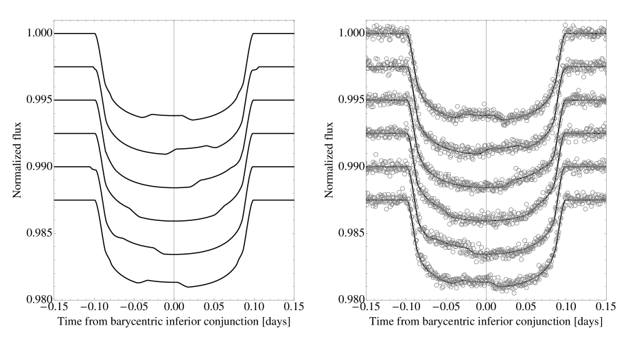
Figure 6: Left panel: Simulation from LUNA of a habitable-zone Neptune with a close, prograde, Earth-like moon for an M2 host star. Right panel: Noised data (circles) of 250 ppm per minute overlaid with best fit from an MCMC routine (solid).

Table 5: Comparison of parameter estimates from various model assumptions used in the fits. Data generated for a Neptune with a close moon around an M2 star.

Parameter	Truth	Prograde	Retrograde	No Moon
$\chi^{2}$	8786.35	8773.48	8775.23	9414.23
BIC	-	8891.31	8893.07	9468.62
Fitted params.
$P_{B*}$ [days]	$46.000000$	$45.999997_{-0.000075}^{+0.000077}$	$46.000000_{-0.000078}^{+0.000080}$	$45.999999_{-0.000085}^{+0.000085}$
$\tau_{B*}$ [BJD - 2454000]	$956.00000$	$956.00001_{-0.00024}^{+0.00023}$	$956.00000_{-0.00024}^{+0.00024}$	$955.99996_{-0.00026}^{+0.00026}$
$p^{2}$ [%]	$0.5071$	$0.5082_{-0.0041}^{+0.0042}$	$0.5082_{-0.0042}^{+0.0042}$	$0.5306_{-0.0027}^{+0.0038}$
$b_{B*}$	$0.00$	$-0.02_{-0.14}^{+0.15}$	$0.02_{-0.14}^{+0.14}$	$0.01_{-0.17}^{+0.16}$
$\tilde{T}_{B*}$ [s]	$15882$	$15877_{-26}^{+26}$	$15877_{-26}^{+26}$	$15895_{-26}^{+26}$
$P_{SB}$ [days]	$0.3142001$	$0.3142029_{-0.0000066}^{+0.0000067}$	$0.3142026_{-0.0000068}^{+0.0000069}$	-
$\phi_{SB}$ [∘]	$40$	$71_{-40}^{+24}$	$21_{-14}^{+12}$	-
$s$	$0.0183$	$0.0181_{-0.0011}^{+0.0011}$	$0.0182_{-0.0011}^{+0.0012}$	$0.0000$
$a_{SB}/R_{*}$	$0.139$	$0.134_{-0.014}^{+0.012}$	$0.129_{-0.015}^{+0.013}$	-
$b_{SB}$	$-0.1$	$-0.21_{-0.95}^{+1.25}$	$0.04_{-0.64}^{+0.58}$	-
$\Omega_{SB}$ [∘]	$5$	$34_{-39}^{+30}$	$-76_{-12}^{+14}$	-
$M_{S}/M_{P}$	$0.058$	$0.073_{-0.020}^{+0.027}$	$0.0694_{-0.018}^{+0.019}$	$0.000$
Physical params.
$M_{*}$ [$M_{\odot}$]	$0.40$	$0.45_{-0.23}^{+0.66}$	$0.69_{-0.39}^{+1.27}$	-
$R_{*}$ [$R_{\odot}$]	$0.50$	$0.52_{-0.11}^{+0.19}$	$0.61_{-0.15}^{+0.25}$	-
$M_{P}$ [$M_{J}$]	$0.054$	$0.057_{-0.022}^{+0.047}$	$0.077_{-0.032}^{+0.076}$	-
$R_{P}$ [$M_{J}$]	$0.346$	$0.363_{-0.078}^{+0.128}$	$0.42_{-0.10}^{+0.17}$	-
$M_{S}$ [$M_{\oplus}$]	$1.00$	$1.31_{-0.58}^{+1.34}$	$1.64_{-0.79}^{+2.08}$	-
$R_{S}$ [$R_{\oplus}$]	$1.00$	$1.03_{-0.22}^{+0.38}$	$1.19_{-0.29}^{+0.54}$	-
$\rho_{S}$ [g cm-3]	$5.5$	$6.5_{-2.2}^{+3.0}$	$5.2_{-1.8}^{+2.2}$	-

We find that all of the parameters from the prograde fit are consistent with the true model. The physical parameters are generally poorly constrained, but apparently sufficient to identify the moon as rocky rather than icy.

4.5 HZ-Neptune with a Far, Retrograde Moon around an M2 Star

4.5.1 Simulation and Fitting

Our second example is identical to the previous one in §4.4, except now we push the orbiting moon into a more distant, retrograde orbit. We place the moon at 90% of the Hill radius (and thus inside the 93.09% limit determined by Domingos et al. (2006)).

4.5.2 Results

A comparison of the fitted parameters for each of our three model assumptions is presented in Table 6, including the $\chi^{2}$ and BIC values of the best-fits for each model. We find that the retrograde moon is only marginally preferable to the prograde model, as expected. However, the no-moon model is clearly a poor fit and would be rejected. An F-test finds the retrograde moon model accepted over no-moon model with a confidence of 50.3-$\sigma$, representing a very secure detection.

The fit assuming a retrograde orbit is shown in the right panel of Figure 7, where the thick black line represents the actual best-fit (i.e. not the original simulation light curve).

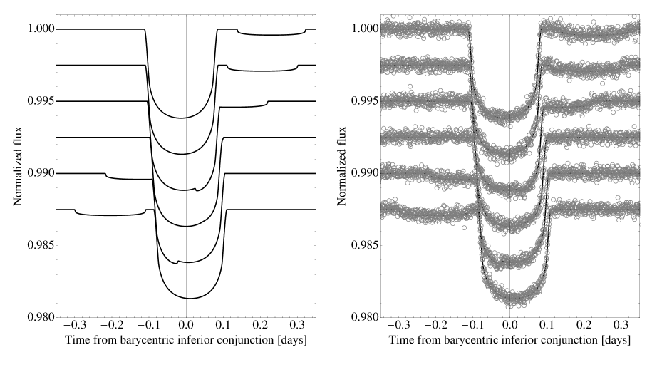
Figure 7: Left panel: Simulation from LUNA of a habitable-zone Neptune with a distant, retrograde, Earth-like moon for an M2 host star. Right panel: Noised data (circles) of 250 ppm per minute overlaid with best fit from an MCMC routine (solid).

Table 6: Comparison of parameter estimates from various model assumptions used in the fits. Data generated for a Neptune with a distant moon around an M2 star.

Parameter	Truth	Retrograde	Prograde	No Moon
$\chi^{2}$	8529.95	8518.65	8518.68	11477.45
BIC	-	8636.48	8636.51	11531.83
Fitted params.
$P_{B*}$ [days]	$46.000000$	$45.99964_{-0.00064}^{+0.00061}$	$45.99967_{-0.00072}^{+0.00058}$	$46.005178_{-0.000085}^{+0.000084}$
$\tau_{B*}$ [BJD - 2454000]	$956.00000$	$956.0010_{-0.0018}^{+0.0019}$	$956.0010_{-0.0017}^{+0.0021}$	$955.98483_{-0.00026}^{+0.00026}$
$p^{2}$ [%]	$0.5071$	$0.5088_{-0.0023}^{+0.0029}$	$0.5088_{-0.0023}^{+0.0029}$	$0.5075_{-0.0028}^{+0.0044}$
$b_{B*}$	$0.00$	$0.02_{-0.14}^{+0.13}$	$0.01_{-0.14}^{+0.14}$	$0.00_{-0.19}^{+0.19}$
$\tilde{T}_{B*}$ [s]	$15882$	$15896_{-26}^{+26}$	$15896_{-26}^{+26}$	$15883_{-27}^{+27}$
$P_{SB}$ [days]	$23.995$	$23.984_{-0.031}^{+0.031}$	$23.987_{-0.034}^{+0.029}$	-
$\phi_{SB}$ [∘]	$40$	$34_{-29}^{+70}$	$143_{-77}^{+46}$	-
$s$	$0.01834$	$0.01842_{-0.00049}^{+0.00048}$	$0.01843_{-0.00049}^{+0.00048}$	$0.00000$
$a_{SB}/R_{*}$	$2.509$	$2.481_{-0.044}^{+0.045}$	$2.478_{-0.044}^{+0.044}$	-
$b_{SB}$	$-0.1$	$-0.02_{-0.83}^{+0.61}$	$-0.09_{-0.59}^{+0.57}$	-
$\Omega_{SB}$ [∘]	$5$	$11_{-70}^{+29}$	$7_{-77}^{+48}$	-
$M_{S}/M_{P}$	$0.0583$	$0.0622_{-0.0070}^{+0.0076}$	$0.0619_{-0.0067}^{+0.0084}$	$0.0000$
Physical params.
$M_{*}$ [$M_{\odot}$]	$0.400$	$0.399_{-0.064}^{+0.061}$	$0.403_{-0.066}^{+0.061}$	-
$R_{*}$ [$R_{\odot}$]	$0.500$	$0.504_{-0.029}^{+0.025}$	$0.506_{-0.029}^{+0.025}$	-
$M_{P}$ [$M_{J}$]	$0.0540$	$0.0537_{-0.0061}^{+0.0055}$	$0.0541_{-0.0063}^{+0.0055}$	-
$R_{P}$ [$M_{J}$]	$0.346$	$0.350_{-0.020}^{+0.018}$	$0.351_{-0.020}^{+0.018}$	-
$M_{S}$ [$M_{\oplus}$]	$1.00$	$1.05_{-0.12}^{+0.13}$	$1.06_{-0.12}^{+0.13}$	-
$R_{S}$ [$R_{\oplus}$]	$1.000$	$1.011_{-0.064}^{+0.059}$	$1.015_{-0.065}^{+0.059}$	-
$\rho_{S}$ [g cm-3]	$5.50$	$5.62_{-0.85}^{+1.03}$	$5.58_{-0.82}^{+1.07}$	-

We find that all of the parameters from the retrograde fit are consistent with the true model. The physical parameters are generally well constrained, in contrast to the close, prograde moon considered in §4.4. This is due to $a_{SB}/R_{*}$ being significantly larger and thus determined to a higher precision which feeds into the other parameters.

4.6 HZ-Neptune without a Moon around an M2 Star

4.6.1 Simulation and Fitting

To complete the picture, we simulate the same case as the previous two subsections but removing the moon altogether. The data are then fitted assuming the three models as before. The purpose of this data set is to show what happens when LUNA is implemented on control data and to ensure such data does not produce false positive moon detections.

4.6.2 Results

A comparison of the fitted parameters for each of our three model assumptions is presented in Table 7, including the $\chi^{2}$ and BIC values of the best-fits for each model. We find that the no-moon model gives the lowest BIC by a considerable margin, as expected. The retrograde and prograde models produce non-sensical values for most parameters, especially the physical parameters, exploring various scenarios with no clear minimum in $\chi^{2}$ space. Note that $s$ and $M_{S}/M_{P}$ are positive definite and therefore are slightly skewed from a zero value, but not significantly so. An F-test finds the retrograde moon model (the best moon fit) accepted over no-moon model with a confidence of 2.0-$\sigma$, which indicates that the detection criterion is clearly in excess of 2-$\sigma$. The use of BIC is therefore more accurate as a model selection tool for exomoon detection.

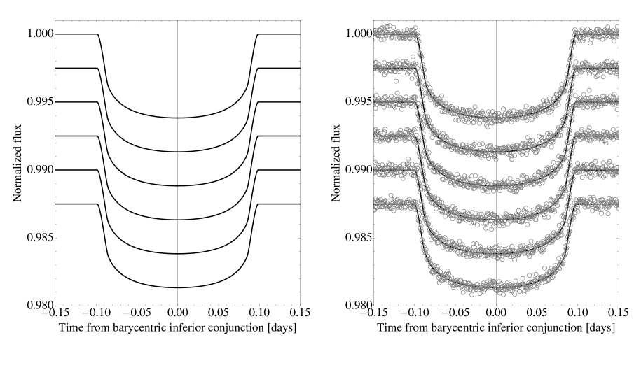
Figure 8: Left panel: Simulation from LUNA of a habitable-zone Neptune with no moon. Right panel: Noised data (circles) of 250 ppm per minute overlaid with best fit from an MCMC routine (solid), from the starting point of assuming a retrograde moon is in orbit.

Table 7: Comparison of parameter estimates from various model assumptions used in the fits. Data generated for a Neptune with no moon around an M2 star.

Parameter	Truth	No Moon	Prograde	Retrograde
$\chi^{2}$	8936.23	8930.96	8928.42	8921.57
BIC	-	8985.34	9046.26	9039.41
Fitted params.
$P_{B*}$ [days]	$46.000000$	$46.000027_{-0.000085}^{+0.000085}$	$46.00001_{-0.00048}^{+0.00057}$
$\tau_{B*}$ [BJD - 2454000]	$956.00000$	$955.99998_{-0.00026}^{+0.00026}$	$956.0000_{-0.0018}^{+0.0015}$	$955.9992_{-0.0076}^{+0.0019}$
$p^{2}$ [%]	$0.5071$	$0.5080_{-0.0026}^{+0.0035}$	$0.005070_{-0.000030}^{+0.000035}$	$0.5065_{-0.0041}^{+0.0037}$
$\tilde{T}_{B*}$ [s]	$15882$	$15883_{-27}^{+27}$	$15881_{-33}^{+32}$	$15883_{-55}^{+66}$
$\phi_{SB}$ [∘]	-	-	$177_{-113}^{+133}$	$223_{-94}^{+84}$
$s$	$0.0000$	$0.0000$	$\leq 0.0094$	$\leq 0.0178$
$a_{SB}/R_{*}$	-	-	$1.15_{-0.57}^{+1.55}$	$1.10_{-0.74}^{+1.86}$
$b_{SB}$	-	-	$-6.0_{-3.4}^{+4.1}$	$-1.6_{-1.9}^{+3.4}$
$\Omega_{SB}$ [∘]	-	-	$4_{-66}^{+59}$	$-16_{-52}^{+79}$
$M_{S}/M_{P}$	$0.00$	$0.00$	$\leq 0.13$	$\leq 0.37$
Physical params.
$M_{*}$ [$M_{\odot}$]	$0.40$	-	$490_{-490}^{+162940}$	$321_{-321}^{+5876270}$
$R_{*}$ [$R_{\odot}$]	$0.50$	-	$5.4_{-5.0}^{+32.0}$	$4.7_{-4.4}^{+119.1}$
$M_{P}$ [$M_{J}$]	$0.054$	-	$6.3_{-6.3}^{+293.1}$	$4.5_{-4.5}^{+3043.3}$
$R_{P}$ [$M_{J}$]	$0.346$	-	$3.7_{-3.4}^{+22.2}$	$3.2_{-3.1}^{+82.2}$
$M_{S}$ [$M_{\oplus}$]	$1.00$	-	$19.4_{-19.4}^{+3644}$	$76_{-76}^{+82460}$
$R_{S}$ [$R_{\oplus}$]	$1.00$	-	$1.4_{-1.3}^{+15.6}$	$1.7_{-1.6}^{+69.3}$
$\rho_{S}$ [g cm-3]	$5.5$	-	$18.5_{-18.4}^{+576.1}$	$79_{-78}^{+5456}$

4.7 General Observations

The simulations above are all for M2 stars with habitable-zone Neptune-like planets and Earth-like moons. These parameters were chosen as Kipping et al. (2009c) have shown that such cases are optimally detectable for habitable-zone scenarios. We also tried the same configurations but using a K5 dwarf ($M_{*}=0.67$ $M_{\odot}$ and $R_{*}=0.72$ $R_{\odot}$) but the longer period of the habitable-zone (half as many transits in the same time window) combined with lower radius and mass ratios for both the planet and moon meant we were unable to find convergent fits. This is not surprising and echoes the motif of the MEarth project (Irwin et al., 2009) and the predictions in Kipping et al. (2009c).

In reviewing our fits, we find that for quantities such as $M_{S}/M_{P}$ and $s$, which are positive definite, an overestimation of their value is common due to the boundary condition that they are greater than zero and the generally low signal-to-noise. This is similar to the situation for orbital eccentricity in radial velocity fits (Lucy & Sweeney, 1971).

5 Discussion & Conclusions

5.1 Comparison to Previous Exomoon Light Curve Simulators

Other works in the scientific literature have made use of algorithms to simulate exomoon transit light curves. To our knowledge, there exists several previous uses of such routines. Figure 4 of Sartoretti & Schneider (1999) presents four simulations of planet-moon combined transits, although details on the methods use to produce these simulations are sparse. Similarly, Szabó et al. (2006) and Simon et al. (2009) present figures with simulated combined transits, although the focus is on a custom definition of transit timing in the former and the effects of the Rossiter-McLaughlin effect in the latter (i.e. few details on the methods use to generate the light curves are provided). Finally, Sato & Asada (2009, 2010) present perhaps the most detailed account of a method to generate planet-moon transit light curves but specifically negate the longitude of the ascending node, orbital inclination of the barycentre, orbital eccentricity of the moon, limb darkening effects and use constant velocity approximations to model the planet/moon motion.

In all cases, there is no reference to the Fewell (2006) solution and we therefore assume this was not utilized in those works. Therefore, all of the previous models must be at least partially numerical in nature since the solution of Fewell (2006) is the first instance of an analytic solution for the area of common overlap between three circles. In contrast, LUNA is fully analytic and we indeed find no appreciable computational time difference between using LUNA versus the usual Mandel & Agol (2002) routine.

5.2 Distinguishing Mutual Events from Starspot Crossings

Visual examination of the simulations presented in §4, in particular Figure 6, reveals that mutual events (i.e. when the planet and moon eclipse one another, during the stellar eclipse) bear a close resemblance to the morphology of a starspot crossing (i.e. when a planet eclipses a starspot on the surface of the star, during the stellar eclipse). Examples of starspot crossing events can be found in Rabus et al. (2009) and Pont et al. (2007). This observation leads to the question as to how one could distinguish between a bona-fide moon and a starspot.

Although a detailed study of this question remains beyond the scope of this work, we suggest here that there are several tools at our disposal to make such a determination. Firstly, starspots are expected to co-rotate with the stellar rotation period, $P_{\mathrm{rot}}$, which can be found by, for example, tracking the long-term flux variation of the target star (e.g. see Henry & Winn 2008). Application of a spot model to the light curve can test whether the spots are consistent with a rotation period determined through other means (Silva-Valio & Lanza, 2011).

A second method we can use is to employ the expressions of Kipping (2010b), which make use of the system dynamics to measure the mass and radius of the host star for exomoon systems. If the determined mass and radius are inconsistent other methods, such as spectroscopy combined with stellar evolution modelling, then it is likely the putative exomoon signal is in fact due to starspots. Whilst a dynamically-determined stellar mass and radius consistent with the spectroscopic value is not a proof of an exomoon, one may evaluate the false-alarm-probability of a starspot coincidentally inducing features which when modelled with LUNA cause precisely the correct stellar mass and radius to be determined. Also, a moon may induce transit timing effects which give rise a derived lunar density which can be compared to expectation.

A third method we suggest is that starspot crossing events will vary in amplitude when viewed chromatically, whereas the exomoon signal will have a chromatic variation much lower (due to atmospheric molecular absorption) and typically undetectable (unless utilizing a telescope such as JWST, see Kipping et al. 2009d). As an example, one could observe the target simultaneously in the visible and infrared wavelengths to test for this chromatic variation.

5.3 Summary

In this paper, we have presented a new algorithm called LUNA for modelling the transit light curves of a single planet with a single moon transiting a star. LUNA was designed from the outset to satisfy several key criteria:

• Analytic (absolutely no numerical components)

• Dynamic (inherently accounts for all timing effects)

• Limb darkening incorporated (including non-linear laws)

• All orbital elements accounted for (e.g. eccentricity, longitude of the ascending node, etc)

As a result of being both precise and analytic, LUNA is a highly potent weapon in exomoon detection. All of the previously predicted observational consequences, such as TTV, TDV-V and TDV-TIP, are inherently built into the routine, plus previously unconsidered effects such as ingress/egress asymmetry. This is done by modelling the reflex motion of the planet due the moon at every instance, which is ultimately responsible for all of the aforementioned timing effects. Transits and mutual eclipses are accounted for using non-linear limb darkening laws meaning LUNA models all known observational consequences of exomoons for transiting systems. Further, physical parameters of the star, planet and moon may be derived utilizing the dynamical trick described in Kipping (2010b).

We have provided simulations of our new algorithm and re-fitted realistic noised data with MCMC methods to demonstrate the inverse retrieval of parameters. In one example, these fits demonstrate that the Kipping (2010b) technique is capable of estimating the stellar mass and radius down to $\sim$15% and $\sim$5% respectively. For the exomoon this becomes $\sim$12% and $\sim$6% respectively. Whilst this is only one singular realization, the simulations lend credence to the prospect of characterizing the internal structure and composition of Earth-mass bodies with current instrumentation. We stress that these examples are primarily to illustrate the effectiveness of our new algorithm rather than estimate the range of configurations which can be conceivably detected, which will be considered in future work.

In this work, we have assumed the moon is small ($R_{S}/R_{*}\ll 1$) but future work will focus on relaxing this constraint so that gas giant binaries may be modelled as well.

Appendix A Planet Moon Motion

A.1 Nested Two-Body Model

We will here derive the relative sky-projected motions of the planet and the moon, as used in the LUNA algorithm. Our goal is to find analytic expressions for the terms $S_{P*}$, $S_{S*}$ and $S_{PS}$, which were introduced in §2.1. We will assume only a single moon in our model and a single planet. To predict the positions of the planet and moon at any instant in time, one must solve the three-body problem. Since no general, analytic solution exists for this problem, one must choose to work in a restricted case where analytic expressions can be employed.

In this work, we will use the nested two-body model presented in Kipping (2010b). This considers the motion of the moon to be independent of the star in the reference frame of the planet-moon barycentre (dubbed the “inner frame”). Therefore, in the inner frame the motions are Keplerian. The barycentre is then considered to also maintain Keplerian motion around the host star in the “outer frame”.

As shown in Kipping (2010b), this model is an excellent approximation for $a_{SB}\lesssim 0.53R_{H}$, where $a_{SB}$ is the moon’s semi-major axis around the planet-moon barycentre and $R_{H}$ is the Hill radius of the planet. Since all bounded prograde satellites must satisfy $a_{SB}\lesssim 0.4895R_{H}$ (Domingos et al., 2006), then the nested two-body model encompasses all prograde moons. We also point out that one may switch the module computing the motions fairly simply, but throughout this paper we will use the nested two-body model.

A.2 Inner Frame

Let us consider the inner frame first, comprising of the planet and moon orbiting a common centre of mass. We define the moon to planet-moon barycentre distance, at any instant in time, as $r_{SB}$. The subscript notation represents S to B or “satellite” to “barycentre” (where barycentre is understood to be the planet-moon barycentre). This notation scheme will be employed throughout this paper so that there exists no ambiguity as to what is being referred to.

$$r_{SB}=|\mathbf{r}_{SB}|=\frac{a_{SB}(1-e_{SB}^{2})}{1+e_{SB}\cos f_{SB}}$$ (45)

Where $a_{SB}$ is the satellite to barycentre semi-major axis, $f_{SB}$ is the true anomaly of the satellite around the barycentre and $e_{SB}$ is eccentricity of the satellite’s orbit around the barycentre.

One of the simplest reference frames in which to view the orbital motion is when the line connecting the apoapse and periapse is the $\hat{x}$-axis and the orbit lies entirely within the $\hat{x}$-$\hat{y}$ plane. Placing the barycentre at the focus lying at $\{a_{SB}e_{S},0,0\}$, the Cartesian coordinates of the satellite are defined by (lower-case symbols are used to denote this is the simple view of the system not yet accounting for an observer’s viewing angle):

$$\mathbf{r}_{SB}=\left(\begin{matrix}x_{SB}\cr y_{SB}\cr z_{SB}\end{matrix}\right)=\left(\begin{matrix}r_{SB}\cos f_{SB}\cr r_{SB}\sin f_{SB}\cr 0\end{matrix}\right)$$ (46)

This is highly analogous to the usual equations describing a planet-star system. In the case of a planet-star, one starts with the analogous version of Equation 46 and then performs three rotations to account for the viewing angle an observer has to the system (Murray & Correia, 2010). These three angles are the argument of periapsis, $\omega$, the orbital inclination, $i$, and the longitude of the ascending node, $\Omega$. The rotations are performed sequentially in a clockwise sense for the $\hat{z}$-$\hat{x}$-$\hat{z}$ axes respectively and are shown in Figure 9.

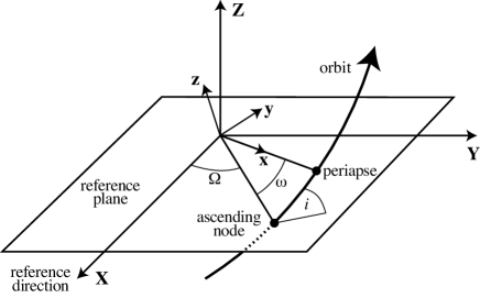
Figure 9: Orbital elements of a two-body system. For a transiting planet-star system, $i\simeq 90^{\circ}$ and the observer is located at $\{X,Y,Z\}=\{0,0,+\infty\}$. Figure from Murray & Correia (2010).

The same scheme will be adopted here for the planet-moon inner frame. For the planet-star case, $i$ is generally close to $\pi/2$ for transits and thus is a large rotation. However, in our case, we choose to perturb the orbit from the coplanar condition. Therefore, we define a small angle for the inclination rotation, $\iota_{SB}$, and use $i_{SB}=\pi/2-\iota_{SB}$ so that $i_{SB}=\pi/2$ corresponds to a coplanar case, in an analogous way to what is used for the planet-star case. The three angles we need to rotate by are $\omega_{SB}$, $\iota_{SB}$ and $\Omega_{SB}$. Murray & Correia (2010) showed that these rotations may be concisely expressed in matrix notation. Following Murray & Correia (2010), we denote the following clockwise rotation matrices about the $\hat{x}$ and $\hat{z}$ axes respectively:

$${\bf P}_{X}(\phi)=\left(\begin{matrix}1&0&0\cr 0&\cos\phi&-\sin\phi\cr 0&\sin\phi&\cos\phi\cr\end{matrix}\right)$$ (47)

$${\bf P}_{Z}(\phi)=\left(\begin{matrix}\cos\phi&-\sin\phi&0\cr\sin\phi&\cos\phi&0\cr 0&0&1\cr\end{matrix}\right)\,.$$ (48)

Armed with these definitions, the transformation from the simple frame of $\{x,y,z\}$ to the observed frame of $\{X,Y,Z\}$ may be written as:

$$\mathbf{R}_{SB}={\bf P}_{Z}(\Omega_{SB}){\bf P}_{X}(\iota_{SB}){\bf P}_{Z}(\omega_{SB})\mathbf{r}_{SB}$$ (49)

After simplification, this yields the following final Cartesian coordinates:

$$X_{SB} =r_{SB}[\cos\Omega_{SB}\cos(\omega_{SB}+f_{SB})$$

$$-\sin i_{SB}\sin\Omega_{SB}\sin(\omega_{SB}+f_{SB})]$$

$$Y_{SB} =r_{SB}[\sin\Omega_{SB}\cos(\omega_{SB}+f_{SB})$$

$$+\sin i_{SB}\cos\Omega_{SB}\sin(\omega_{SB}+f_{SB})]$$

$$Z_{SB} =r_{SB}\cos i_{SB}\sin(\omega_{SB}+f_{SB})$$ (50)

Note that $R_{SB}=|\mathbf{R}_{SB}|=|\mathbf{r}_{SB}|=r_{SB}$. The planet’s reflex motion can be found by simply using:

$$\mathbf{R}_{PB}M_{P}+\mathbf{R}_{SB}M_{S}=0$$ (51)

A.3 Outer Frame

To obtain the overall motion, we now need to account for motion of the planet-moon barycentre around the star. Placing the star at the origin, the barycentre-star separation, at any instant, is given by:

$$r_{B*}=|\mathbf{r}_{B*}|=\frac{a_{B*}(1-e_{B*}^{2})}{1+e_{B*}\cos f_{B*}}$$ (52)

Where $a_{B*}$ is the barycentre to star semi-major axis (usually just dubbed $a$), $f_{B*}$ is the true anomaly of the barycentre around the star (usually just dubbed $f$) and $e_{B*}$ is eccentricity of the barycentre’s orbit around the star (usually just dubbed $e$).

In exactly the same way as was done in the inner frame, the barycentre’s position can be described in a simple frame which is then rotated to account for the viewing angle of the observer. The simple frame has the barycentre at Cartesian coordinates:

$$\mathbf{r}_{B*}=\left(\begin{matrix}x_{B*}\cr y_{B*}\cr z_{B*}\end{matrix}\right)=\left(\begin{matrix}r_{B*}\cos f_{B*}\cr r_{B*}\sin f_{B*}\cr 0\end{matrix}\right)$$ (53)

This is then rotated in the same way as before:

$$\mathbf{R}_{B*}={\bf P}_{Z}(\Omega_{B*}){\bf P}_{X}(i_{B*}){\bf P}_{Z}(\omega_{B*})\mathbf{r}_{B*}$$ (54)

The last rotation, about $\hat{z}$ by $\Omega_{B*}$, has no bearing on the transit because the light curve is defined by the star-planet separation only, which is invariant about a $\hat{z}$-axis rotation since the observer lies at $z=+\infty$. For this reason, there is no need to include this final angle in practice:

$$\mathbf{R}_{B*}={\bf P}_{X}(i_{B*}){\bf P}_{Z}(\omega_{B*})\mathbf{r}_{B*}$$ (55)

To compute the Cartesian coordinates of the planet and moon (rather than the planet-moon barycentre), we need to combine the results of the inner frame derivation with the process of the outer frame. This is achieved by considering that:

$$\mathbf{r}_{S*} =\mathbf{R}_{SB}+\mathbf{r}_{B*}$$ (56)

$$\mathbf{r}_{P*} =\mathbf{R}_{PB}+\mathbf{r}_{B*}$$ (57)

The conversion from $\mathbf{r}_{S*}\rightarrow\mathbf{R}_{S*}$ is performed by repeating the rotations used to go from $\mathbf{r}_{B*}\rightarrow\mathbf{R}_{B*}$ (and similarly for $\mathbf{r}_{P*}$). This gives:

$$\mathbf{R}_{S*}={\bf P}_{Z}(\Omega_{B*}){\bf P}_{X}(i_{B*}){\bf P}_{Z}(\omega_{B*})(\mathbf{R}_{SB}+\mathbf{r}_{B*})$$ (58)

$$\mathbf{R}_{P*}={\bf P}_{Z}(\Omega_{B*}){\bf P}_{X}(i_{B*}){\bf P}_{Z}(\omega_{B*})(\mathbf{R}_{PB}+\mathbf{r}_{B*})$$ (59)

Evaluating, this gives the satellite’s position as:

$$X_{S*} =r_{B*}\cos(f_{B*}+\omega_{B*})$$

$$+r_{SB}\cos(f_{SB}+\omega_{SB})\cos(\omega_{B*}+\Omega_{SB})$$

$$-r_{SB}\sin i_{SB}\sin(f_{SB}+\omega_{SB})\sin(\omega_{B*}+\Omega_{SB})$$ (60)

$$Y_{S*} =r_{B*}\cos i_{B*}\sin(f_{B*}+\omega_{B*})$$

$$-r_{SB}\sin i_{B*}\cos i_{SB}\sin(f_{SB}+\omega_{SB})$$

$$+r_{SB}\cos i_{B*}\sin i_{SB}\cos(\omega_{B*}+\Omega_{SB})\sin(f_{SB}+\omega_{SB})$$

$$+r_{SB}\cos i_{B*}\sin(\omega_{B*}+\Omega_{SB})\cos(f_{SB}+\omega_{SB})$$ (61)

$$Z_{S*} =r_{B*}\sin i_{B*}\sin(f_{B*}+\omega_{B*})$$

$$+r_{SB}\cos i_{B*}\cos i_{SB}\sin(f_{SB}+\omega_{SB})$$

$$+r_{SB}\sin i_{B*}\sin i_{SB}\cos(\omega_{B*}+\Omega_{SB})\sin(f_{SB}+\omega_{SB})$$

$$+r_{SB}\sin i_{B*}\sin(\omega_{B*}+\Omega_{SB})\cos(f_{SB}+\omega_{SB})$$ (62)

Evaluating for the planet, we find:

$$X_{P*} =r_{B*}\cos(f_{B*}+\omega_{B*})$$

$$-r_{PB}\cos(f_{SB}+\omega_{SB})\cos(\omega_{B*}+\Omega_{SB})$$

$$+r_{PB}\sin i_{SB}\sin(f_{SB}+\omega_{SB})\sin(\omega_{B*}+\Omega_{SB})$$ (63)

$$Y_{P*} =r_{B*}\cos i_{B*}\sin(f_{B*}+\omega_{B*})$$

$$+r_{PB}\sin i_{B*}\cos i_{SB}\sin(f_{SB}+\omega_{SB})$$

$$-r_{PB}\cos i_{B*}\sin i_{SB}\cos(\omega_{B*}+\Omega_{SB})\sin(f_{SB}+\omega_{SB})$$

$$-r_{PB}\cos i_{B*}\sin(\omega_{B*}+\Omega_{SB})\cos(f_{SB}+\omega_{SB})$$ (64)

$$Z_{P*} =r_{B*}\sin i_{B*}\sin(f_{B*}+\omega_{B*})$$

$$-r_{PB}\cos i_{B*}\cos i_{SB}\sin(f_{SB}+\omega_{SB})$$

$$-r_{PB}\sin i_{B*}\sin i_{SB}\cos(\omega_{B*}+\Omega_{SB})\sin(f_{SB}+\omega_{SB})$$

$$-r_{PB}\sin i_{B*}\sin(\omega_{B*}+\Omega_{SB})\cos(f_{SB}+\omega_{SB})$$ (65)

A.4 Sky-Projected Distances

The usual planetary transit light curve is completely described by the sky-projected distance between the planet and the star. In the same way, the light curve of a planet with a moon is described by the sky-projected distances, defined as $S=\sqrt{X^{2}+Y^{2}}/R_{*}$ (units of the stellar radius are used). Using $r_{B*}^{\prime}=r_{B*}/R_{*}$, $r_{SB}^{\prime}=r_{SB}/R_{*}$ and $r_{PB}^{\prime}=r_{PB}/R_{*}$, the sky-projected moon-star distance is:

$$S_{S*}^{2} =\Big{[}r_{B*}^{\prime}\cos(f_{B*}+\omega_{B*})+r_{SB}^{\prime}\cos(\omega_{B*}+\Omega_{SB})\cos(f_{SB}+\omega_{SB})$$

$$-r_{SB}^{\prime}\sin i_{SB}\sin(\omega_{B*}+\Omega_{SB})\sin(f_{SB}+\omega_{SB})\Big{]}^{2}$$

$$+\Big{[}r_{B*}^{\prime}\cos i_{B*}\sin(f_{B*}+\omega_{B*})$$

$$-r_{SB}^{\prime}\cos i_{SB}\sin i_{B*}\sin(f_{SB}+\omega_{SB})$$

$$+r_{SB}^{\prime}\cos i_{B*}\sin i_{SB}\cos(\omega_{B*}+\Omega_{SB})\sin(f_{SB}+\omega_{SB})$$

$$+r_{SB}^{\prime}\cos i_{B*}\sin(\omega_{B*}+\Omega_{SB})\cos(f_{SB}+\omega_{SB})\Big{]}^{2}$$ (66)

And for the planet:

$$S_{P*}^{2} =\Big{[}r_{B*}^{\prime}\cos(f_{B*}+\omega_{B*})-r_{PB}^{\prime}\cos(\omega_{B*}+\Omega_{SB})\cos(f_{SB}+\omega_{SB})$$

$$+r_{PB}^{\prime}\sin i_{SB}\sin(\omega_{B*}+\Omega_{SB})\sin(f_{SB}+\omega_{SB})\Big{]}^{2}$$

$$+\Big{[}r_{B*}^{\prime}\cos i_{B*}\sin(f_{B*}+\omega_{B*})$$

$$+r_{PB}^{\prime}\cos i_{SB}\sin_{B*}\sin(f_{SB}+\omega_{SB})$$

$$-r_{PB}^{\prime}\cos i_{B*}\sin i_{SB}\cos(\omega_{B*}+\Omega_{SB})\sin(f_{SB}+\omega_{SB})$$

$$-r_{PB}^{\prime}\cos i_{B*}\sin(\omega_{B*}+\Omega_{SB})\cos(f_{SB}+\omega_{SB})\Big{]}^{2}$$ (67)

Another important term is the separation between the planet and moon alone:

$$S_{SP}^{2} =\frac{(X_{P*}-X_{S*})^{2}+(Y_{P*}-Y_{S*})^{2}}{R_{*}^{2}}$$

$$S_{SP}^{2} =[r_{PB}^{\prime}+r_{SB}^{\prime}]^{2}\Bigg{(}\Big{[}\cos(\omega_{B*}+\Omega_{SB})\cos(f_{SB}+\omega_{SB})$$

$$-\sin i_{SB}\sin(\omega_{B*}+\Omega_{SB})\sin(f_{SB}+\omega_{SB})\Big{]}^{2}$$

$$+\Big{[}\sin i_{B*}\cos i_{SB}\sin(f_{SB}+\omega_{SB})$$

$$-\cos i_{B*}\sin i_{SB}\cos(\omega_{B*}+\Omega_{SB})\sin(f_{SB}+\omega_{SB})$$

$$-\cos i_{B*}\sin(\omega_{B*}+\Omega_{SB})\cos(f_{SB}+\omega_{SB})\Big{]}^{2}\Bigg{)}$$ (68)

A.5 Repeating Units

Inspection of the above equations reveals several repeating units. Substituting these units allows for a more simple and intuitive expression of the sky projected distances. The following two units repeat in all three sky projected distances:

$$\beta =r_{SB}^{\prime}\Big{[}\cos(\omega_{B*}+\Omega_{SB})\cos(f_{SB}+\omega_{SB})$$

$$-\sin i_{SB}\sin(\omega_{B*}+\Omega_{SB})\sin(f_{SB}+\omega_{SB})\Big{]}$$ (69)

$$\gamma =r_{SB}^{\prime}\Big{[}\cos i_{B*}\sin i_{SB}\cos(\omega_{B*}+\Omega_{SB})\sin(f_{SB}+\omega_{SB})$$

$$+\cos i_{B*}\sin(\omega_{B*}+\Omega_{SB})\cos(f_{SB}+\omega_{SB})$$

$$-\sin i_{B*}\cos i_{SB}\sin(f_{SB}+\omega_{SB})\Big{]}$$ (70)

Using these substitutions, the sky-projected distances are simplified to:

$$S_{S*} =[r_{B*}^{\prime}\cos(f_{B*}+\omega_{B*})+\beta]^{2}$$

$$+[r_{B*}^{\prime}\cos i_{B*}\sin(f_{B*}+\omega_{B*})+\gamma]^{2}$$ (71)

$$S_{P*} =[r_{B*}^{\prime}\cos(f_{B*}+\omega_{B*})-(M_{S}/M_{P})\beta]^{2}$$

$$+[r_{B*}^{\prime}\cos i_{B*}\sin(f_{B*}+\omega_{B*})-(M_{S}/M_{P})\gamma]^{2}$$ (72)

$$S_{SP} =[1+(M_{S}/M_{P})]^{2}[\beta^{2}+\gamma^{2}]$$ (73)

The substitution terms may be split into terms which vary with time and those which do not, using a matrix $\mathbf{I}$ defined as the “inner” matrix:

$$\mathbf{I}=\begin{bmatrix}\beta\\ \gamma\end{bmatrix}=\begin{bmatrix}\beta_{1}&\beta_{2}\\ \gamma_{1}&\gamma_{2}\end{bmatrix}\begin{bmatrix}\sin(f_{SB}+\omega_{SB})\\ \cos(f_{SB}+\omega_{SB})\end{bmatrix}$$ (74)

Where:

$$\beta_{1} =-r_{s}^{\prime}\sin i_{SB}\sin(\omega_{B*}+\Omega_{SB})$$ (75)

$$\beta_{2} =r_{s}^{\prime}\cos(\omega_{B*}+\Omega_{SB})$$ (76)

$$\gamma_{1} =r_{s}^{\prime}[\cos i_{B*}\sin i_{SB}\cos(\omega_{B*}+\Omega_{SB})-\sin i_{B*}\cos i_{SB}]$$ (77)

$$\gamma_{2} =r_{s}^{\prime}\cos i_{B*}\sin(\omega_{B*}+\Omega_{SB})$$ (78)

As the matrix form provides a natural way to describe the motions, it is convenient to extend it to the barycentric motion as well:

$$S_{S*}^{2} =[\mathbf{O}_{2}+\mathbf{I}_{1}]^{2}+[\mathbf{O}_{1}+\mathbf{I}_{2}]^{2}$$ (79)

$$S_{P*}^{2} =[\mathbf{O}_{2}-(M_{S}/M_{P})\mathbf{I}_{1}]^{2}+[\mathbf{O}_{1}-(M_{S}/M_{P})\mathbf{I}_{2}]^{2}$$ (80)

Where:

$$\mathbf{O}_{1} =\psi=r_{B*}^{\prime}\cos i_{B*}\sin(f_{B*}+\omega_{B*})+0$$

$$=\psi_{1}\sin(f_{B*}+\omega_{B*})+\psi_{2}\cos(f_{B*}+\omega_{B*})$$ (81)

$$\mathbf{O}_{2} =\epsilon=0+r_{B*}^{\prime}\cos(f_{B*}+\omega_{B*})$$

$$=\epsilon_{1}\sin(f_{B*}+\omega_{B*})+\epsilon_{2}\cos(f_{B*}+\omega_{B*})$$ (82)

Where we have used:

$$\psi_{1} =r_{B*}^{\prime}\cos i_{B*}$$ (83)

$$\psi_{2} =0$$ (84)

$$\epsilon_{1} =0$$ (85)

$$\epsilon_{2} =r_{B*}^{\prime}$$ (86)

Here, $\psi_{1}=b_{B*}$, the impact parameter of the barycentre across the face of the star, and $\epsilon_{2}=a_{B*}/R_{*}$ for a circular orbit. These two parameters are typically fitted for in planetary light curve analysis, but it is widely known that they share a strong correlation. In matrix form we have the “outer” matrix as:

$$\mathbf{O}=\begin{bmatrix}\psi\\ \epsilon\end{bmatrix}=\begin{bmatrix}\psi_{1}&0\\ 0&\epsilon_{2}\end{bmatrix}\begin{bmatrix}\sin(f_{B*}+\omega_{B*})\\ \cos(f_{B*}+\omega_{B*})\end{bmatrix}$$ (87)

References

- Carter et al. (2008) Carter, J. A., Yee, J. C., Eastman, J., Gaudi, B. S. & Winn, J. N., 2008, ApJ, 689, 499
- Claret (2000) Claret, A. 2000, A&A, 363, 1081
- Cox (2000) Cox, A. N. (ed.), Allen’s Astrophysical Quantities (4th edition) (Springer, Heidelberg), 2000
- Domingos et al. (2006) Domingos, R. C., Winter, O. C. & Yokoyama, T. 2006, MNRAS, 373, 1227
- Donnison (2010) Donnison J. R., 2010, MNRAS, 406, 1918
- Fewell (2006) Fewell, M., “Area of Common Overlap of Three Circles”, Tech. Rep. DSTO-TN-0722, 2006. [Online]. Available: http://hdl.handle.net/1947/4551
- Han & Han (2002) Han, C. & Han, W. 2002, ApJ, 580, 490
- Henry & Winn (2008) Henry, G. W., & Winn, J. N. 2008, AJ, 135, 68
- Irwin et al. (2009) Irwin, J., Charbonneau, D., Nutzman, P. & Falco, E. 2009, in IAU Symp. 253, Transiting Planets, ed. F. Pont, D. Sasselov, & M. Holman (Cambridge: Cambridge Univ. Press), 37
- Kipping (2008) Kipping, D. M., 2008, MNRAS, 389, 1383
- Kipping (2009a) Kipping, D. M., 2009a, MNRAS, 392, 181
- Kipping (2009b) Kipping, D. M., 2009b, MNRAS, 396, 1797
- Kipping et al. (2009c) Kipping, D. M., Fossey, S. J. & Campanella, G., 2009c, MNRAS, 400, 398
- Kipping et al. (2009d) Kipping, D. M., Fossey, S. J., Campanella, G., Schneider, J., & Tinetti, G. 2009d, in ASP Conf. Ser. 430, Pathways Towards Habitable Planets, ed. V. C. du Foresto, D. M. Gelino, & I. Ribas (San Francisco, CA: ASP), 139
- Kipping (2010a) Kipping, D. M., 2010a, MNRAS, 407, 301
- Kipping (2010b) Kipping, D. M. 2010b, MNRAS Letters, 409, L119
- Kipping (2011) Kipping, D. M. 2011, PhD thesis, University College London
- Kipping & Bakos (2011a) Kipping, D. M. & Bakos, G., 2011a, ApJ, 730, 50
- Kipping & Bakos (2011b) Kipping, D. M. & Bakos, G., 2011b, ApJ, 733, 36
- Kurucz (2006) Kurucz R., 2006, Stellar Model and Associated Spectra (http://kurucz.harvard.edu/grids.html)
- Lewis et al. (2008) Lewis, K. M., Sackett, P. D. & Mardling, R. A. 2008, ApJ, 685, 153
- Liddle et al. (2007) Liddle, A. R. 2007, MNRAS, 377, L74
- Lovis et al. (2011) Lovis, C. et al. 2011, A&A, 528, 112
- Lucy & Sweeney (1971) Lucy, L. B. & Sweeney, M. A. 1971, AJ, 76, 544
- Mandel & Agol (2002) Mandel, K. & Agol, E. 2002, ApJ, 580, L171
- Murray & Dermott (1999) Murray, C. D. & Dermott, S. F. (1999), Solar System Dynamics, Cambridge University Press, Cambridge
- Murray & Correia (2010) Murray, C. D. & Correia, A. C. M. 2010, EXOPLANETS, eds. S. Seager, University of Arizona Press
- Pont et al. (2007) Pont, F. et al. 2007, A&A, 476, 1347
- Rabus et al. (2009) Rabus, M. et al. 2009, A&A, 494, 391
- Sartoretti & Schneider (1999) Sartoretti, P. & Schneider, J., 1999, A&AS, 134, 553
- Sato & Asada (2009) Sato, M. & Asada, H. 2009, PASJ, 61, L29
- Sato & Asada (2010) Sato, M. & Asada, H. 2009, PASJ, 62, 1203
- Schwarz (1978) Schwarz, G. 1978, The Annals of Statistics, 6, 461
- Silva-Valio & Lanza (2011) Silva-Valio, A. & Lanza, A. F. 2011, A&A, 529, 36
- Simon et al. (2009) Simon, A., Szabó, Gy. M. & Szatmáry, K. 2009, EM&P, 105, 385
- Szabó et al. (2006) Szabó, Gy. M., Szatmáry, K., Divéki, Zs. & Simon, A. 2006, A&A, 2006, 450, 395
- Vogt et al. (2010) Vogt, S. S., Butler, R. P., Rivera, E. J., Haghighipour, N., Henry, G. W. & Williamson, M. H. 2010, ApJ, 723, 954