The structure function of variable 1.4 GHz radio sources based on NVSS and FIRST observations

Abstract

We augment the two widest/deepest 1.4 GHz radio surveys: the NRAO VLA Sky Survey (NVSS) and the Faint Images of the Radio Sky at Twenty-Centimeters (FIRST), with the mean epoch in which each source was observed. We use these catalogs to search for unresolved sources which vary between the FIRST and NVSS epochs. We find 43 variable sources (0.1% of the sources) which vary by more than 4$\sigma$, and we construct the mean structure function of these objects. This enables us to explore radio variability on time scales between several months and about five years. We find that on these time scales, the mean structure function of the variable sources is consistent with a flat structure function. A plausible explanation to these observations is that a large fraction of the variability at 1.4 GHz is induced by scintillations in the interstellar medium, rather than by intrinsic variability. Finally, for a sub sample of the variables for which the redshift is available, we do not find strong evidence for a correlation between the variability amplitude and the source redshift.

1. Introduction

Variability of radio sources at low frequencies is mainly attributed to propagation effects (scintillations) induced by large scale electron density inhomogeneities in the Inter-Stellar Medium (ISM; e.g., Hunstead 1972; Rickett, Coles & Bourgois 1984; Rickett 1990; Ghosh & Rao 1992). The predicted variability structure function of compact radio sources due to scintillations (e.g., Blandford & Narayan 1985; Goodman & Narayan 1985; Blandford et al. 1986; Hjellming & Narayan 1986) is roughly consistent with the typically observed structure function, at least below 5 GHz (e.g., Qian et al. 1995; Gaensler & Hunstead 2000). These models predict a rise in the structure function up to time scales of $\sim 10$ days at $\approx 5$ GHz and up to $\sim 100$ days at $\approx 0.5$ GHz, followed by a flattening of the structure function.

Specifically, Qian et al. (1995) analyzed radio observations of the compact radio source 1741$-$038 ($z=1.054$) taken in several frequencies between 1.5 and 22 GHz. They compared the observed structure functions with theoretical models for scattering by an extended Galactic medium, with and without a thin screen component. They reported that for frequencies below about 5 GHz the observations are consistent with a scattering by an extended Galactic medium and a thin screen. However, above this frequency they found excess variability relative to the models. Moreover, at these high frequencies, the structure function continues to rise towards longer time scales. They suggested that at high frequencies ($\mathrel{\raise 1.29167pt\hbox{$>$}\mkern-14.0mu\lower 2.58334pt\hbox{$\sim$}}5$ GHz) some of the variability of this radio source is intrinsic. This general picture is also supported by Mitchell et al. (1994).

Gaensler & Hunstead (2000) studied the variability of 55 radio calibrators observed by the Molonglo Observatory Synthesis Telescope (MOST) at 843 MHz. They constructed the structure function for 18 variable sources. For the majority of these variable objects the structure function flattens on time scales of a few hundreds days. Furthermore, they confirmed early results (Condon et al. 1979) which found that the variability amplitude is increasing as a function of the source spectral index $\alpha$, defined by $f_{\nu}\propto\nu^{\alpha}$, where $f_{\nu}$ is the specific flux at frequency $\nu$. This is attributed to a correlation between the source angular size and spectral index. Another confirmation for the importance of Galactic scintillations is that radio variability depends on Galactic latitude (e.g., Spangler et al. 1989; Ghosh & Rao 1992; Gaensler & Hunstead 2000). We note however that Rys & Machalski (1990) did not find evidence for increasing fraction of 1.4 GHz variability for sources brighter than 100 mJy at low Galactic latitudes.

Lovell et al. (2008) presented results from the Micro-Arcsecond Scintillation-Induced Variability (MASIV) survey conducted at 5 GHz. Among their findings: half of the sources they monitored exhibit 2%–10% rms variations on time scales over two days. They also found that the structure function of the variable sources rises on time scales of a few days, and the variability amplitudes correlates with the H$\alpha$ emission at the direction of the sources. Furthermore, there is evidence that the variability amplitude decrease with redshift above $z\approx 2$, presumably due to evolution of the source size with redshift (see however Lazio et al. 2008).

Here we compare the two widest/deepest 1.4 GHz sky surveys taken using the Very Large Array (VLA), and search for variable sources. We use these datasets to construct the average structure function on time scales between several months and about five years and to look for indications for intrinsic variability of these sources. In §2 we present augmented versions of the FIRST and NVSS catalogs which contains the mean time in which each source was observed. In §3 we cross correlate the two catalogs, and in §4 we construct the structure function of the variable sources. Finally, we discuss the results in §5.

2. The catalogs

The NVSS observations were carried out between June 1993 and April 1999, while the FIRST survey observations were conducted between March 1993 and September 2002. Therefore, these observations provide a long baseline to the structure function analysis. Constructing the structure function of variable sources requires knowledge of their fluxes at multiple epochs and the time at which the observations were taken. However, the NRAO VLA Sky Survey (NVSS; Condon et al. 1998) and the Faint Images of the Radio Sky at Twenty-Centimeters (FIRST; Becker et al. 1995) source catalogs do not contain the time at which each source was observed. The reason for this is that the observing times are not well defined. Images in both surveys were taken by scanning the sky in a hexagonal grid in which observing points are separated by $26^{\prime}$. Both surveys were obtained using the VLA, in which the full width at half power at 1.4 GHz is $\cong 31^{\prime}$. Each primary beam field of view was truncated to radii of $24^{\prime}$ and $23.5^{\prime}$ for the NVSS and FIRST surveys, respectively. Therefore, each point on the sky effectively contains information from roughly four different pointings taken at different times.

In order to obtain the epoch at which each source was observed we downloaded from the VLA archive the list of all observing scans which are associated with each sky survey.

Next, we cross-correlate the list of observing scans for each project with its catalog of sources. We use a matching radii equal to the truncation radii of $24^{\prime}$ and $23.5^{\prime}$ for the NVSS and FIRST surveys, respectively. This enable us to estimate for each source, the number of observations ($N_{{\rm obs}}$), its mean observing time (over all scan mid times, $t_{{\rm ep}}$) and the time span within which these observation were obtained ($\delta{t}$).

The products are versions of the FIRST and NVSS catalogs that contains the observing time, number of observations, and time span of observations for each source. In Tables 1–2 we present a version of these catalogs containing the source coordinates and the observing time information for each source.

Table 1Observing times of NVSS sources

J2000 RA	J2000 Dec	$f$	$\sigma_{{\rm f}}$	$N_{{\rm obs}}$	$t_{{\rm ep}}$	$\delta{t}$
deg	deg	mJy	mJy		days	days
194.89704	$-40.37908$	3.60	0.70	1	0220.698	0.000
249.00512	$-40.37366$	99.70	3.60	1	0220.840	0.000
199.42008	$-40.36441$	24.30	1.20	1	0220.699	0.000
248.90470	$-40.36169$	3.00	0.60	1	0220.840	0.000
212.86787	$-40.35236$	2.70	0.50	1	0220.737	0.000

Note. — A version of the NVSS catalog containing the source position, mean observing time ($t_{{\rm ep}}$), number of scans ($N_{{\rm obs}}$), and the time span over which the scans were obtained ($\delta{t}$). The observing time, $t_{{\rm ep}}$, is given in ${\rm JD}-2450000$ days, where JD is the Julian day. $f$ is the peak flux density and $\sigma_{{\rm f}}$ is the error in the peak flux density. We note that our cross correlation of the observing scans and the sources catalog was not able to produce the observing times of 591 sources. This table is published in its entirety in the electronic edition of the Astrophysical Journal. A portion of the full table is shown here for guidance regarding its form and content. The table is sorted by Declination, therefore the sources listed here are near the edge of the survey footprint and have a single observation.

Table 2Observing times of FIRST sources

J2000 RA	J2000 Dec	$f$	$\sigma_{{\rm f}}$	$N_{{\rm obs}}$	$t_{{\rm ep}}$	$\delta{t}$
deg	deg	mJy	mJy		days	days
354.74904	$-11.39882$	1.68	0.14	1	0593.087	0.000
5.19669	$-11.39761$	1.02	0.15	1	0593.118	0.000
6.82096	$-11.39611$	1.11	0.15	1	0595.073	0.000
359.90417	$-11.39585$	1.39	0.15	1	0593.102	0.000
6.70133	$-11.39458$	1.17	0.14	1	0595.073	0.000

Note. — Like Table 1 but for the FIRST catalog. We note that our cross correlation of the observing scans and the sources catalog was not able to produce the observing times of 379 sources.

Figure 1 presents histograms of the number of individual snapshots used to compose each source image. For both surveys, the typical number of snapshots per composite image is 3–4 (see also Helfand et al. 1996). In Figure 2 we show histograms of $\delta{t}$ for the two surveys. This figure suggests that most of the images are made from snapshots taken within a few weeks range of each other.

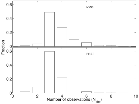
Figure 1.— Histogram of number of observations from which each source image was composed. Bin size is 1 observation. The upper panel is for NVSS sources, while the lower panel is for FIRST sources.

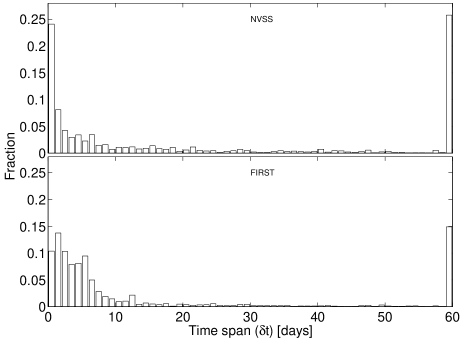
Figure 2.— Histogram of the time span of observations from which each source image was composed ($\delta{t}$). Bin size is 1 day. Panels like in Fig. 1. The last bin on the right-hand side is for all $\delta{t}>59$ days.

We note that a transient search based on the comparison of the FIRST and NVSS catalogs was presented in Levinson et al. (2002) and discussed in Gal-Yam et al. (2006) and Ofek et al. (2010). However, these previous efforts did not use the observing time of the sources.

3. Cross correlation of the FIRST and NVSS catalogs

The FIRST catalog contains 816,331 sources, brighter than about $1$ mJy, mainly in the North Galactic cap. About $81$% of these sources have $\delta{t}<30$ days. The NVSS catalog contains 1,773,484 objects with $\delta>-30$ deg, brighter than about $3.5$ mJy, of which $\cong 67$% have $\delta{t}<30$ days. We select all the FIRST sources which deconvolved major and minor axes equal zero (i.e., point sources), the peak flux density is larger than 5 mJy, all the scans composing their flux measurement ($\delta{t}$) were taken within 30 days, and which are isolated from any other FIRST source (of any kind) within $60^{\prime\prime}$. Since the resolution of the NVSS is $45^{\prime\prime}$, nine times coarser than that of the FIRST survey, the last step is designed to remove NVSS sources which flux may be contaminated by multiple FIRST objects. We found 6463 FIRST sources that satisfy these criteria. Next, from the NVSS catalog we select all sources with $\delta{t}<30$ days – we find 1,183,620 sources that satisfy this criterion.

Then, for each object in the subset of the FIRST catalog we search for a source in the subset of the NVSS catalog which is found within $15^{\prime\prime}$ of the FIRST object. We found 4367 matched sources. These matches represent point sources for which we have both a FIRST and NVSS flux-density measurements. We note that only $68\%$ of the FIRST sources in this list have NVSS matches. This is mostly due to the fact that we used only NVSS sources with $\delta{t}<30$ days.

Next, we would like to compare the fluxes of unresolved NVSS and FIRST sources. However, systematic biases in the NVSS and/or FIRST flux calibration could effect our analysis. Condon et al. (1998) and Becker et al. (1995) discussed photometric errors such as the CLEAN bias, and they made corrections to their source catalogs flux densities. For both the NVSS and FIRST catalogs the CLEAN bias is $\approx-0.3$ mJy, i.e. of order the rms noise in the images. There is also a well-known discrepancy between integrated fluxes of extended sources in FIRST and NVSS, owing to resolution effects (Blake & Wall 2002). In Figure 3 we show the mean of the peak-flux ratio between matched individual NVSS and FIRST point sources, as a function of flux density (black circles).

This figure suggests that at the faint end, NVSS fluxes are systematically lower than FIRST fluxes. Blake & Wall (2002) already reported this effect, although with an opposite direction and higher amplitude. However, Blake & Wall (2002) looked at both resolved and unresolved sources, while we are interested only in point sources. Probably the most important reason for this trend is related to the fact that the NVSS and FIRST surveys have different resolutions. Another secondary effect is a bias similar to the Eddington bias (Eddington 1913). This is because sources which flux expectancy value is smaller than 5 mJy (our FIRST flux cut) and are detected in the FIRST survey above 5 mJy (due to measurement errors) have $>50$% chance to have an NVSS flux density below 5 mJy. This effect is amplified by the fact that faint sources are more common, per unit flux density, than bright sources. The estimated amplitude of this bias, based on simulations, is shown by the gray line in Figure 3.

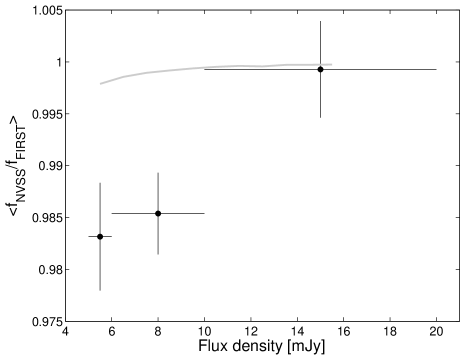
Figure 3.— The mean of the flux ratio between matched individual NVSS and FIRST point sources, as a function of flux density (black circles). The horizontal “error bars” represent the bin size in which the mean flux ratio was measured. The expected amplitude of the Eddington-like bias (see text) is shown in gray line.

Given these results we correct the NVSS fluxes of the matched point sources by the amount interpolated from the black circles in Figure 3. Above 20 mJy we assume that the correction factor is 1. We neglect the effect of the Eddington bias, since its expected amplitude is negligible (see Fig. 3). We note that the maximum amplitude of the applied correction is smaller than the rms noise in the NVSS measurements and comparable to rms noise of FIRST sources. A caveat in our bias analysis is that this bias may also depend on the actual angular extent of the unresolved sources. Therefore, the bias expectation value for a given flux may depends on a “hidden” parameter which value is not measured, and cannot be entirely removed from the data.

The FIRST vs. NVSS peak flux-density measurements of the matched point sources are presented in Figure 4.

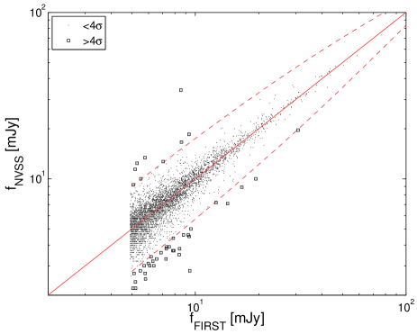
Figure 4.— The FIRST peak specific flux vs. the same quantity from the NVSS catalog for the 4367 matched unresolved sources (see text). The solid line shows the 1:1 line, while the dashed lines represent $4\sigma$ below and above the 1:1 line. Open boxes shows the 43 sources that are variable by more than $4\sigma$, while all the other matched sources are marked by dots. We note that there are more variable sources below the lower line than above the upper line (see text).

Based on this plot we estimate the standard deviation, $\sigma$, of the differences between FIRST and NVSS specific fluxes as a function of FIRST flux. This is done by calculating the 68-percentile range in the flux-flux plot as a function of the FIRST flux density, $f_{{\rm FIRST}}$. We divide the 68 percentile by $2$ to estimate the standard deviation, and then fit a first order polynomial to the logarithm of the standard deviation estimator as a function of flux density. We find that the relative errors associated with these difference measurements are well represented by

$$\sigma/f\approx 10^{-0.6652-0.0064f_{{\rm FIRST}}}.$$ (1)

Here we define variables as objects for which the FIRST vs. NVSS flux difference is larger than $4\sigma$. We found 43 such variable sources, which are listed in Table 3. We inspected the radio images of all these variable sources by eye, and comments on individual sources appear in this table. We note that the theoretical errors are smaller, and have different functional forms, than those implied by Equation 1. However, in order to avoid any possible uncertainties in the comparison between the two catalogs, we used the empirical errors.

Although we attempt to correct for the flux bias between FIRST and NVSS sources, in Figure 4 there are more variable sources below the lower 4-$\sigma$ line than above the upper 4-$\sigma$ line. This systematic difference may be related to the complexity of the bias between the FIRST and NVSS measurements, mentioned earlier. Effectively, this systematic bias induces errors in the number of “sigmas” in which a source is variable. However, the ratio of number of sources above the upper 4-$\sigma$ line to that below the lower 4-$\sigma$ line, is consistent with an additional systematic shift in the flux ratio of $\approx 0.35\sigma$. Therefore, we conclude that since we used a relatively large variability threshold of 4$\sigma$, most of our variable sources are probably real.

4. The structure function

Next, we calculate the mean structure function for all the 43 sources which exceed the 4-$\sigma$ variability threshold in Figure 4. As a reference we also calculated the structure function for all the 3906 “non-variable” sources defined here as sources which variability is less than $2\sigma$.

Table 3Variable sources

J2000.0					USNO-B1		2MASS			ROSAT	SDSS
RA	Dec	$f_{{\rm FIRST}}$	$f_{{\rm NVSS}}$	$\Delta{t}$	$B_{2}$	$R_{2}$	$J$	$H$	$K$	Dist	$g$	$r$	$z_{{\rm sp}}$	$z_{{\rm ph}}$
deg	deg	mJy	mJy	day	mag	mag	mag	mag	mag	′′	mag	mag
229.95525	$-5.90828$	$19.40\pm 0.14$	$10.0\pm 0.5$	$1736.7$	$\cdots$	$\cdots$	$\cdots$	$\cdots$	$\cdots$	$\cdots$	$\cdots$	$\cdots$	$\cdots$	$\cdots$
34.81875	$-4.64270$	$5.72\pm 0.14$	$3.0\pm 0.7$	$1270.9$	$\cdots$	$\cdots$	$\cdots$	$\cdots$	$\cdots$	$\cdots$	$\cdots$	$\cdots$	$\cdots$	$\cdots$
208.61233	$0.73462$	$5.20\pm 0.18$	$2.4\pm 0.5$	$760.9$	$\cdots$	$\cdots$	$\cdots$	$\cdots$	$\cdots$	$\cdots$	$\cdots$	$\cdots$	$\cdots$	$\cdots$
120.64970	$7.55780$	$5.19\pm 0.15$	$11.4\pm 1.5$	$1758.9$	$\cdots$	$\cdots$	$\cdots$	$\cdots$	$\cdots$	$\cdots$	$\cdots$	$\cdots$	$\cdots$	$\cdots$
193.96310	$8.74396$	$7.90\pm 0.19$	$3.7\pm 0.4$	$1288.4$	$\cdots$	$\cdots$	$\cdots$	$\cdots$	$\cdots$	$\cdots$	24.70	22.76	$\cdots$	0.30
158.12037	$8.98541$	$8.60\pm 0.15$	$16.6\pm 0.6$	$1719.3$	19.6	18.5	$\cdots$	$\cdots$	$\cdots$	$\cdots$	19.28	19.28	0.454	0.45
155.94935	$10.65521$	$5.77\pm 0.15$	$13.4\pm 1.6$	$1698.6$	$\cdots$	$\cdots$	$\cdots$	$\cdots$	$\cdots$	$\cdots$	24.42	22.33	$\cdots$	$\cdots$
225.14947	$13.45289$	$6.08\pm 0.14$	$3.0\pm 0.4$	$1271.5$	$\cdots$	20.0	$\cdots$	$\cdots$	$\cdots$	$\cdots$	23.01	21.37	$\cdots$	$\cdots$
114.80608	$18.03965$	$7.26\pm 0.16$	$3.3\pm 0.5$	$1762.5$	17.1	16.9	16.14	15.49	14.86	$\cdots$	17.36	17.12	$\cdots$	1.00
201.32666	$19.46406$	$7.04\pm 0.14$	$12.7\pm 0.5$	$1712.8$	$\cdots$	$\cdots$	$\cdots$	$\cdots$	$\cdots$	$\cdots$	$\cdots$	$\cdots$	$\cdots$	$\cdots$
206.50009	$19.73055$	$5.78\pm 0.15$	$2.7\pm 0.4$	$1702.0$	$\cdots$	$\cdots$	$\cdots$	$\cdots$	$\cdots$	$\cdots$	24.12	23.18	$\cdots$	$\cdots$
244.32375	$20.57935$	$7.82\pm 0.14$	$3.7\pm 0.4$	$1320.1$	$\cdots$	$\cdots$	$\cdots$	$\cdots$	$\cdots$	$\cdots$	22.70	22.29	$\cdots$	$\cdots$
222.17540	$20.67543$	$6.88\pm 0.15$	$3.6\pm 0.5$	$1322.1$	$\cdots$	$\cdots$	$\cdots$	$\cdots$	$\cdots$	$\cdots$	$\cdots$	$\cdots$	$\cdots$	$\cdots$
247.57423	$23.33178$	$9.41\pm 0.36$	$2.8\pm 0.4$	$286.9$	20.9	19.7	$\cdots$	$\cdots$	$\cdots$	$\cdots$	20.87	20.52	$\cdots$	2.60
212.99535	$23.89795$	$9.53\pm 0.14$	$5.0\pm 0.4$	$284.4$	$\cdots$	$\cdots$	$\cdots$	$\cdots$	$\cdots$	$\cdots$	22.19	21.96	$\cdots$	$\cdots$
252.75117	$24.26111$	$8.79\pm 0.14$	$4.6\pm 0.4$	$197.4$	$\cdots$	$\cdots$	$\cdots$	$\cdots$	$\cdots$	$\cdots$	22.86	21.67	$\cdots$	$\cdots$
190.23317	$24.33961$	$5.80\pm 0.15$	$2.5\pm 0.4$	$284.2$	$\cdots$	$\cdots$	$\cdots$	$\cdots$	$\cdots$	$\cdots$	$\cdots$	$\cdots$	$\cdots$	$\cdots$
182.98029	$25.36394$	$5.48\pm 0.15$	$2.8\pm 0.4$	$213.8$	20.2	20.5	$\cdots$	$\cdots$	$\cdots$	$\cdots$	20.83	20.66	$\cdots$	0.30
247.48198	$27.72523$	$7.28\pm 0.16$	$3.8\pm 0.5$	$183.4$	$\cdots$	19.7	$\cdots$	$\cdots$	$\cdots$	$\cdots$	22.40	20.78	$\cdots$	$\cdots$
238.73764	$29.95945$	$5.08\pm 0.14$	$9.2\pm 1.0$	$-754.7$	18.9	18.7	$\cdots$	$\cdots$	$\cdots$	$\cdots$	18.89	18.87	0.855	0.85
203.08994	$29.99894$	$16.62\pm 0.59$	$8.9\pm 1.1$	$-745.7$	$\cdots$	$\cdots$	$\cdots$	$\cdots$	$\cdots$	$\cdots$	$\cdots$	$\cdots$	$\cdots$	$\cdots$
136.90323	$30.25872$	$9.35\pm 0.15$	$4.5\pm 0.5$	$-286.1$	$\cdots$	$\cdots$	$\cdots$	$\cdots$	$\cdots$	$\cdots$	22.13	21.99	$\cdots$	$\cdots$
203.03348	$30.69115$	$9.26\pm 1.35$	$4.6\pm 0.5$	$-735.7$	$\cdots$	$\cdots$	$\cdots$	$\cdots$	$\cdots$	$\cdots$	$\cdots$	$\cdots$	$\cdots$	$\cdots$
169.75685	$36.87706$	$9.33\pm 0.15$	$18.5\pm 1.1$	$-289.7$	16.3	15.7	15.98	15.25	14.60	$\cdots$	25.12	19.25	$\cdots$	$\cdots$
170.99205	$38.43646$	$6.17\pm 0.15$	$3.4\pm 0.4$	$-260.7$	$\cdots$	$\cdots$	$\cdots$	$\cdots$	$\cdots$	$\cdots$	$\cdots$	$\cdots$	$\cdots$	$\cdots$
122.43647	$38.50171$	$7.86\pm 0.14$	$4.4\pm 0.5$	$202.8$	$\cdots$	$\cdots$	$\cdots$	$\cdots$	$\cdots$	$\cdots$	$\cdots$	$\cdots$	$\cdots$	$\cdots$
119.02080	$39.25484$	$6.36\pm 0.14$	$3.0\pm 0.4$	$218.6$	19.2	17.6	$\cdots$	$\cdots$	$\cdots$	$\cdots$	20.45	19.62	$\cdots$	$\cdots$
262.32334	$44.77948$	$5.98\pm 0.14$	$3.1\pm 0.5$	$700.7$	$\cdots$	$\cdots$	$\cdots$	$\cdots$	$\cdots$	$\cdots$	$\cdots$	$\cdots$	$\cdots$	$\cdots$
229.90208	$44.97024$	$5.12\pm 0.15$	$2.7\pm 0.4$	$710.8$	$\cdots$	$\cdots$	$\cdots$	$\cdots$	$\cdots$	$\cdots$	24.15	23.91	$\cdots$	0.10
134.99454	$45.87719$	$30.74\pm 0.15$	$19.6\pm 0.7$	$1207.4$	19.2	18.6	$\cdots$	$\cdots$	$\cdots$	$\cdots$	18.86	19.05	0.440	0.50
220.45533	$50.71170$	$5.06\pm 0.16$	$2.2\pm 0.4$	$753.7$	$\cdots$	$\cdots$	$\cdots$	$\cdots$	$\cdots$	$\cdots$	$\cdots$	$\cdots$	$\cdots$	$\cdots$
262.65758	$52.24396$	$7.32\pm 0.14$	$3.9\pm 0.4$	$766.6$	$\cdots$	$\cdots$	16.57	15.86	15.01	$\cdots$	$\cdots$	$\cdots$	$\cdots$	$\cdots$
211.65318	$52.68479$	$8.42\pm 0.22$	$3.8\pm 0.4$	$772.9$	$\cdots$	$\cdots$	$\cdots$	$\cdots$	$\cdots$	$\cdots$	$\cdots$	$\cdots$	$\cdots$	$\cdots$
159.71340	$53.49093$	$8.53\pm 0.15$	$34.1\pm 1.8$	$765.5$	19.9	$\cdots$	$\cdots$	$\cdots$	$\cdots$	53.2	$\cdots$	$\cdots$	$\cdots$	$\cdots$
226.56440	$53.92288$	$5.30\pm 0.15$	$12.4\pm 1.1$	$770.9$	21.6	$\cdots$	$\cdots$	$\cdots$	$\cdots$	$\cdots$	21.75	21.57	$\cdots$	2.40
179.14175	$54.63838$	$12.54\pm 0.27$	$7.2\pm 0.5$	$779.5$	$\cdots$	$\cdots$	$\cdots$	$\cdots$	$\cdots$	$\cdots$	$\cdots$	$\cdots$	$\cdots$	$\cdots$
157.78099	$56.75153$	$6.56\pm 0.18$	$3.3\pm 0.4$	$780.2$	20.6	18.9	$\cdots$	$\cdots$	$\cdots$	$\cdots$	20.84	19.82	$\cdots$	$\cdots$
157.96070	$56.85260$	$6.29\pm 0.20$	$3.2\pm 0.4$	$780.2$	$\cdots$	$\cdots$	$\cdots$	$\cdots$	$\cdots$	$\cdots$	$\cdots$	$\cdots$	$\cdots$	$\cdots$
160.55682	$59.35609$	$5.51\pm 0.15$	$10.0\pm 0.9$	$2642.4$	$\cdots$	$\cdots$	$\cdots$	$\cdots$	$\cdots$	$\cdots$	$\cdots$	$\cdots$	$\cdots$	$\cdots$
151.08074	$59.53517$	$8.38\pm 0.16$	$3.5\pm 0.4$	$3075.2$	$\cdots$	$\cdots$	$\cdots$	$\cdots$	$\cdots$	$\cdots$	$\cdots$	$\cdots$	$\cdots$	$\cdots$
185.45517	$61.59247$	$7.51\pm 0.15$	$3.9\pm 0.4$	$2655.3$	$\cdots$	$\cdots$	$\cdots$	$\cdots$	$\cdots$	$\cdots$	23.10	21.16	$\cdots$	$\cdots$
248.86649	$62.64994$	$14.23\pm 1.51$	$7.1\pm 1.1$	$2665.3$	$\cdots$	$\cdots$	$\cdots$	$\cdots$	$\cdots$	$\cdots$	$\cdots$	$\cdots$	$\cdots$	$\cdots$
124.64543	$63.90501$	$5.21\pm 0.14$	$2.2\pm 0.4$	$3192.3$	$\cdots$	$\cdots$	$\cdots$	$\cdots$	$\cdots$	$\cdots$	$\cdots$	$\cdots$	$\cdots$	$\cdots$

Note. — List of 43 sources which vary by more than 4$\sigma$ between the FIRST and NVSS epochs. The table is sorted by declination. Columns description: $f$ is the peak specific flux and its error. The subscript indicate the catalog name. $\Delta{t}$ is the time between the FIRST and NVSS observations. The position of each source was cross correlated with various catalogs, including the USNO-B1 (Monet al. 2003), 2MASS (Skrutskie et al. 2006), ROSAT bright and faint source catalogs (Voges et al. 1999; Voges et al. 2000), and the Sloan Digital Sky Survey (York et al. 2000). In case counterparts are found we list their USNO-B1 $B_{2}$ and $R_{2}$ magnitudes, 2MASS $J$, $H$ and $K$ magnitudes, distance from ROSAT source, and SDSS $g$ and $r$ magnitudes and redshifts. We use search radius, relative to the FIRST catalog position, of $60^{\prime\prime}$ for ROSAT and $2.5^{\prime\prime}$ for all the other catalogs. $z$ is the SDSS spectroscopic redshift of the source, while $z_{{\rm ph}}$ is the photometric redshift of the source based on the SDSS colors. We use a photometric redshift estimator for quasars which is described in Ofek et al. (2002). The photometric redshift is calculated only if the source is indicated as a possible quasar in the SDSS database. We note that non of these sources are associated with a GB6 source (e.g., Gregory et al. 1996) or a known pulsar.

Comments on individual sources:
RA$=155.94935$ deg, Dec$=+10.65521$ deg : The peak flux we measure in the NVSS image is a factor of two lower than the flux stated in the NVSS catalog, so this may be a constant source.

RA$=247.57423$ deg, Dec$=+23.33178$ deg : Near the strong source 3C 340 – NVSS and FIRST images are noisy.

RA$=203.03348$ deg, Dec$=+30.69115$ deg : Radio images are noisy.

RA$=159.71340$ deg, Dec$=+53.49093$ deg : This is possibly a radio SN in the outskirts of NGC 3310 (Argo et al. 2004).

RA$=226.56440$ deg, Dec$=+53.92288$ deg : NVSS image shows a double source.

RA$=157.78099$ deg, Dec$=+56.75153$ deg : Extended emission 15 arcmin from source.

RA$=157.96070$ deg, Dec$=+56.85260$ deg : Extended emission 4 arcmin from source.

RA$=124.64543$ deg, Dec$=+63.90501$ deg : FIRST flux may be influenced by sidelobes from 3C 343 (4.5 Jy, 9 arcmin to the NW).

The structure function was calculated according to the following scheme. For each pair of matched FIRST and NVSS measurements, we calculate the time difference between the FIRST ($t_{{\rm ep}}^{{\rm FIRST}}$) and NVSS ($t_{{\rm ep}}^{{\rm NVSS}}$) epochs: $\Delta{t_{i}}=t_{{\rm ep}}^{{\rm FIRST}}-t_{{\rm ep}}^{{\rm NVSS}}$. Here, $i$ is the index of the pair. We also calculate for each pair

$$\Delta{f_{i}}/\bar{f}_{i}=\frac{f_{{\rm NVSS},i}-\bar{f}_{i}}{\bar{f}_{i}},$$ (2)

where $f_{{\rm NVSS},i}$ and $f_{{\rm FIRST},i}$ are the NVSS and FIRST specific fluxes of the $i$-th source, and $\bar{f}_{i}=(f_{{\rm NVSS},i}+f_{{\rm FIRST},i})/2$. Next, the structure function and its error are estimated in bins of 500 days, between zero and 3500 days, by calculating the mean and standard deviation of $\Delta{f_{i}}/\bar{f}_{i}$ for all the pairs $i$ in the appropriate bin.

Figure 5 shows the structure function for the variable (black) and non variable (gray) sources.

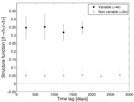
Figure 5.— The structure function of variable sources (black circles) and non-variable sources (gray circles) as a function of time lag. The measurements are displayed only for bins in which the number of flux differences is larger than four. The errors are based on the standard deviation in each bin. The horizontal dashed line marks the zero structure function.

The structure function in this time range is consistent with being flat, with mean relative variability of about 35%. However, the value of 35% probably represents our sensitivity for variability rather than some physical variability level. The only physically interesting fact is the flatness of the structure function.

5. Discussion

We present versions of the FIRST and NVSS catalogs that contain the mean epoch in which each source was observed. We use these catalogs to look for variable sources, and we construct the structure function for these objects. We show that the structure function is flat on time scales between about half a year and five years.

It is well known that the structure function of variable radio sources rises on time scales of days to tens of days (e.g., Qian et al. 1995; Gaensler & Hunstead 2000; Lovell et al. 2008; Ofek et al. 2011). Intrinsic variability of compact radio sources, which are mainly Active Galactic Nuclei (AGN), on days time scales would imply that the sources have small physical size. This in turn requires a very high rest-frame brightness temperature ($T_{{\rm B,rest}}$), orders of magnitude above $\sim 10^{12}$ K which is the limit for an incoherent synchrotron source (e.g., Kellermann & Pauliny-Toth 1969; Readhead 1994). Therefore, most or all of the variability of radio sources, below $\sim 5$ GHz, on these short time scales is presumably due to scintillations in the ISM. Moreover, based on causality arguments, intrinsic variability of compact radio sources is expected only on time scales ($\tau_{V}$) larger than

$$\tau_{V} \mathrel{\raise 1.29167pt\hbox{$>$}\mkern-14.0mu\lower 2.58334pt\hbox{$\sim$}} 50\Big{(}\frac{\Delta{f}}{1\,{\rm mJy}}\Big{)}^{1/2}\Big{(}\frac{d_{{\rm lum}}}{6.7\,{\rm Gpc}}\Big{)}\Big{(}\frac{\nu}{1.4\,{\rm GHz}}\Big{)}^{-1}$$ (4)

$$\times\Big{(}\frac{\mathcal{D}}{10}\Big{)}^{-3/2}\Big{(}\frac{1+z}{2}\Big{)}^{3/2}\Big{(}\frac{T_{{\rm B,rest}}}{10^{12}\,{\rm K}}\Big{)}^{-1/2}\,{\rm day},$$

where $\Delta{f}$ is the variation amplitude in specific flux, $d_{{\rm lum}}$ is the luminosity distance (normalized at $z\cong 1$), $\mathcal{D}$ is the Doppler factor of a relativistic motion in the source, and $z$ is the source redshift. In Equation 4, $T_{{\rm B,rest}}$ is given in the rest frame and all the other parameters are in the observer reference frame. We note that Eq. 4 is derived from the relation for the brightness temperature, and replacing the source size by $c\tau_{V}$, where $c$ is the speed of light.

In contrast, observations of quasars and BL Lac objects performed in the 4.8–14.5 GHz range showed that the structure function saturates only on time scales between a year and ten years (Hughes, Aller & Aller 1992). Therefore, the fact that we do not see any significant rise in the structure function on time scales of months to years suggests that, at 1.4 GHz, the amplitude of intrinsic variability relative to scintillations is small. Alternatively, it may suggest that the 1.4 GHz power spectrum of AGN radio variability is consistent with a white-noise power spectrum, rather than the red-noise power spectrum typically seen at shorter wavelengths (e.g., Giveon et al. 1999; Markowitz et al. 2003). We note that Padrielli et al. (1987) reported on a class of sources (denoted “C-BBV” in their terminology) which show correlated intrinsic variability in low (0.4 GHz) and high (14.5 GHz) frequencies. However, these sources are a minority among the variable sources in their sample.

Figure 6 shows the fraction of variables as a function of Galactic latitude.

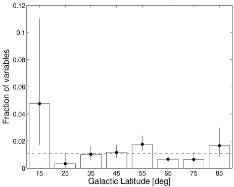
Figure 6.— The fraction of variables, relative to all the non-variable and variable sources, as a function of Galactic latitude. The error bars represent the 1-$\sigma$ errors on the fractions (Gehrels 1986). The dashed horizontal line marks the mean “all-sky” fraction of variables in our sample (i.e., $43/3949=0.0109$).

The first bin contains two variables out of 42 objects (a fraction of 0.048). However, the expectation value in this bin, estimated based on the mean fraction of variables (dashed line in Fig. 6; $0.0109$) multiplied by the number of sources in the first bin (42) is 0.457. Assuming a binomial distribution, the cumulative probability to observe $\geq 2$ events, given an expectation value of 0.457, is 7.7%. This rules out the null hypothesis that the low-latitude variable-fraction is drawn from a uniform all-sky distribution at the 92.3% confidence. Therefore, a larger sample is required in order to confirm the earlier claims that the fraction of variables is larger at low Galactic latitude (e.g., Gaensler & Hunstead 2000). If this excess is real, then a plausible explanation is that it is due to ISM scintillations which are more prominent at low Galactic latitudes. However, we cannot rule out that some of this excess in variability is due to a population of Galactic variable sources as suggested by Becker et al. (2010).

Finally, we use our dataset to look for correlation of the variability amplitude with redshift. There are several factors that can contribute to such a correlation. For example, scintillations depends on the source angular size (larger amplitude for smaller sources), intrinsic source size evolution, broadening due to scattering, and maybe even scintillation in the intra-galactic medium (which may depends on the He re-ionization). Figure 7 shows $\Delta{f_{i}}/\bar{f}_{i}$ as a function of redshift for all nine variable sources for which we have a redshift estimate (Table 3).

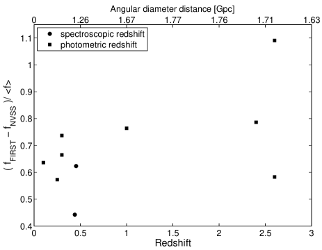
Figure 7.— The variability relative amplitude, $\Delta{f_{i}}/\bar{f}_{i}$, as a function of redshift for all nine variable sources that are quasars or quasar candidates (Table 3). The upper x-axis shows the angular diameter distance corresponding to the redshift, assuming WMAP fifth year cosmological parameters (Komatsu et al. 2009).

The Spearman rank (Pearson) correlation coefficient between the redshift and the relative variability amplitude is 0.59 (0.79). In order to estimate the significance of this correlation we conduct $10^{4}$ bootstrap simulations (Efron 1982; Efron & Tibshirani 1993). In each simulation we select, for each source redshift, a random variability amplitude from the list of nine amplitudes. We find that the probability to get a Spearman rank correlation coefficient $>0.59$ is about 5%. Therefore, unlike Lovell et al. (2008) we do not find any strong evidence for correlation between scintillations and redshift. However, our sample is considerably smaller than the one presented by Lovell et al. (2008). We note that eight out of the nine sources in Figure 7 are found above Galactic latitude of 40 deg, and one source is at Galactic latitude of about 18 deg. Removing the single low galactic latitude source (the source at $z\approx 1$ in Figure 7) reduces the Spearman rank correlation to 0.42 and therefore does not change this results significantly.

References

- Argo et al. (2004) Argo, M. K., Muxlow, T. W. B., Pedlar, A., Beswick, R. J., & Strong, M. 2004, MNRAS, 351, L66
- Becker et al. (1995) Becker, R. H., White, R. L., & Helfand, D. J. 1995, ApJ, 450, 559
- Becker et al. (2010) Becker, R. H., Helfand, D. J., White, R. L., & Proctor, D. D. 2010, arXiv:1005.1572
- Blake & Wall (2002) Blake, C., & Wall, J. 2002, MNRAS, 337, 993
- Blandford & Narayan (1985) Blandford, R., & Narayan, R. 1985, MNRAS, 213, 591
- Blandford et al. (1986) Blandford, R., Narayan, R., & Romani, R. W. 1986, ApJL, 301, L53
- Condon et al. (1979) Condon, J. J., Ledden, J. E., Odell, S. L., & Dennison, B. 1979, AJ, 84, 1
- Condon et al. (1998) Condon, J. J., Cotton, W. D., Greisen, E. W., Yin, Q. F., Perley, R. A., Taylor, G. B., & Broderick, J. J. 1998, AJ, 115, 1693
- Eddington (1913) Eddington, A. S. 1913, MNRAS, 73, 359
- Efron (1982) Efron, B., 1982, The Jackknife, the Bootstrap and Other Resampling Plans, The Society for Industrial and Applied Mathematics
- ET (1993) Efron, B., Tibshirani, R.J., 1993, An introduction to the bootstrap, Monographs on statistics and applied probability 57, Chapman & Hall