Barycentric Hermite Interpolation

Abstract.

Let $z_{1},\ldots,z_{K}$ be distinct grid points. If $f_{k,0}$ is the prescribed value of a function at the grid point $z_{k}$, and $f_{k,r}$ the prescribed value of the $r$-th derivative, for $1\leq r\leq n_{k}-1$, the Hermite interpolant is the unique polynomial of degree $N-1$ ($N=n_{1}+\cdots+n_{K}$) which interpolates the prescribed function values and function derivatives. We obtain another derivation of a method for Hermite interpolation recently proposed by Butcher et al. [Numerical Algorithms, vol. 56 (2011), p. 319-347]. One advantage of our derivation is that it leads to an efficient method for updating the barycentric weights. If an additional derivative is prescribed at one of the interpolation points, we show how to update the barycentric coefficients using only $\mathcal{O}\left(N\right)$ operations. Even in the context of confluent Newton series, a comparably efficient and general method to update the coefficients appears not to be known. If the method is properly implemented, it computes the barycentric weights with fewer operations than other methods and has very good numerical stability even when derivatives of high order are involved. We give a partial explanation of its numerical stability.

1. Introduction

An example of a Hermite interpolant in barycentric form is the unique polynomial $\pi(z)$ of degree $3$ such that $\pi(-1)=f_{-1}$, $\pi^{\prime}(-1)=f_{-1}^{{}^{\prime}}$, $\pi(1)=f_{1}$, and $\pi^{\prime}(1)=f_{1}^{{}^{\prime}}$ as given by

(1.1) $$\pi(z) = (z-1)^{2}(z+1)^{2}\Biggl{(}f_{-1}\left(\frac{1}{4(z+1)^{2}}+\frac{1}{4(z+1)}\right)+\frac{f_{-1}^{{}^{\prime}}}{4(z+1)}$$

$$+f_{1}\left(\frac{1}{4(z-1)^{2}}-\frac{1}{4(z-1)}\right)+\frac{f_{1}^{{}^{\prime}}}{4(z-1)}\Biggr{)}.$$

In general Hermite interpolation, the function value and its first $n_{k}-1$ derivatives are prescribed as

$$f_{k,0},\ldots,f_{k,n_{k}-1}$$

at the interpolation point or grid point $z_{k}$ for each $z_{k}$ from the list $z_{1},\ldots,z_{K}$. The problem is to find a polynomial $\pi(z)$ of degree $N-1$, where $N=n_{1}+\cdots+n_{K}$, such that

(1.2) $$\frac{d^{r}\pi(z)}{dz^{r}}\Biggl{|}_{z=z_{k}}=f_{k,r}\quad\text{for}\quad r=0,\ldots,n_{k}-1$$

at each grid point $z_{k}$. We shall always assume the grid points $z_{k}$ to be distinct. For an elegant proof of the existence and uniqueness of the Hermite interpolant, see [6].

The polynomial $\pi(z)$ can be represented in either the Newton form or the barycentric form. In the Newton form, the grid points $z_{k}$ must be ordered in some way [4]. If the grid points are not carefully ordered, the Newton form is susceptible to catastrophic numerical instability [7, 17]. In contrast, the barycentric form does not require the grid points to be ordered and treats all the grid points equally.

Barycentric form. The barycentric form of the interpolant is

(1.3) $$\begin{split}\pi(z)=\pi^{\ast}(z)\sum_{k=1}^{K}\frac{f_{k,n_{k}-1}}{(n_{k}-1)!}\left(\frac{w_{k,0}}{(z-z_{k})}\right)+\frac{f_{k,n_{k}-2}}{(n_{k}-2)!}\left(\frac{w_{k,0}}{(z-z_{k})^{2}}+\frac{w_{k,1}}{(z-z_{k})}\right)+\cdots\\ +f_{k,0}\left(\frac{w_{k,0}}{(z-z_{k})^{n_{k}}}+\cdots+\frac{w_{k,n_{k}-1}}{(z-z_{k})}\right)\end{split}$$

where $\pi^{\ast}(z)$ is defined as $\prod_{k=1}^{K}(z-z_{k})^{n_{k}}$. It is evident from inspection that $\pi(z)$, as represented in (1.3), is a polynomial of degree $N-1$. For a unique choice of weights $w_{k,r}$, $\pi(z)$ will satisfy the interpolation conditions (1.2). Determining and updating the weights (or coefficients) $w_{k,r}$ of the barycentric form is the topic of this paper.

The representation of $\pi(z)$ shown in (1.3) is usually termed the first barycentric form. For the second barycentric form, take $f_{k,0}=1$ and $f_{k,r}=0$ for $r\geq 1$ corresponding to the function $f(z)=1$. By the existence and uniqueness of the Hermite interpolant, we have $1=\pi^{\ast}(z)\sum_{k=1}^{K}\sum_{r=0}^{n_{k}-1}w_{k,r}(z-z_{k})^{n_{k}-r}$. Dividing (1.3) by the barycentric representation of $1$, we have

(1.4) $$\pi(z)=\frac{\sum_{k=1}^{K}\sum_{s=0}^{n_{k}-1}\frac{f_{k,s}}{s!}\sum_{r=0}^{n_{k}-s-1}w_{k,r}(z-z_{k})^{n_{k}-r-s}}{\sum_{k=1}^{K}\sum_{r=0}^{n_{k}-1}w_{k,r}(z-z_{k})^{n_{k}-r}}.$$

This is the second barycentric form. The second barycentric form has a useful property that we now state. If the first barycentric form (1.3) satisfies the interpolation conditions (1.2), so does the second barycentric form (1.4). Less obviously, for any choice of the weights $w_{k,r}$ with $w_{k,0}\neq 0$ for $k=1,\ldots,K$, the second barycentric form is a rational function of $z$ which satisfies the interpolation conditions (1.2) (see [13]and [1]). The second barycentric form is more robust in the presence of rounding errors in the weights $w_{k,r}$ , as one may expect and as we will demonstrate in Section 4.

For deriving the weights $w_{k,r}$, we shall work with the first barycentric form (1.3). It is obvious from inspection that either of the two forms can be used to evaluate the interpolant $\pi(z)$ at a given point $z$ using $\mathcal{O}(N)$ arithmetic operations, although the second barycentric form is more robust in the presence of rounding errors.

Calculating barycentric weights using divided differences. One of the methods for finding the weights $w_{k,r}$ in $\mathcal{O}(N^{2})$ operations is due to Schneider and Werner [13]. Two ideas go into that method. We briefly describe the two ideas in the simpler context of Lagrange interpolation (see Werner [20] for this special case) where the problem is to find a polynomial $p(z)$ of degree $K-1$ such that $p(z_{k})=f_{k,0}$ holds at each grid point $z_{k}$.

The Newton representation of $p(z)$ is $a_{0}+a_{1}(z-z_{1})+a_{2}(z-z_{1})(z-z_{2})+\cdots+a_{K-1}\prod_{k<K}(z-z_{k})$ for some coefficients $a_{k}$. The Lagrange representation takes the form $\sum_{k=1}^{K}b_{k}L_{k}(z)$, where $L_{k}(z)$ is the un-normalized Lagrange cardinal function $\prod_{j\neq k}(z-z_{j})$. The first idea is to note that the coefficients $a_{k}$ and the coefficients $b_{k}$ are connected by a triangular matrix [10]. The second idea is to note that if $p(z)\equiv 1$ then $a_{0}=1$ and $a_{k}=0$ for $k\geq 1$ and the coefficients $b_{k}$ are equal to the Lagrange weights $w_{k}$. The triangular relationship between the two sets of coefficients is inverted using divided differences to compute the Lagrange weights. The method of Schneider and Werner for computing the barycentric weights $w_{k,r}$ of the Hermite interpolant follows the same logic.

We make two comments about the method of Schneider and Werner. Firstly, because the Newton expansion is used implicitly, the method depends upon divided differences and finding a good ordering of the grid points $z_{k}$. Even if the grid points are carefully ordered and scaled using the logarithmic capacity of the interval of interpolation, it is unclear from the extant literature if the method is numerically stable in the presence of high order derivatives. As our discussion in Sections 4 and 5 will indicate, numerical stability is a more delicate issue when high order derivatives occur in the Hermite data.

Secondly, the method for finding barycentric weights described in Section 2 typically has a lower operation count than the method of divided differences. However, Schneider and Werner [13] allow a general denominator in the barycentric form while we specialize the denominator to be $1$. Even though it could be possible to specialize the method of divided differences to lower the operation count, that is unlikely to make it a better method for computing the barycentric weights. The argument for the method of Section 2 is its simplicity, directness, and numerical stability.

The method of Butcher et al. [3] and its extension. In Section 2, we give another derivation of the method of Butcher et al. for computing the barycentric weights. The method was derived by Butcher et al. using contour integrals and the manipulation of infinite series. Our derivation is more direct. The formalism of Butcher et al. extends to Birkhoff interpolation (or Hermite interpolation with incomplete data), a problem which is not discussed here.

To explain the basic idea we use in Section 2 for computing the barycentric weights, we go back to the Hermite interpolant shown in (1.1). We want to compute a cubic polynomial whose Taylor expansion to two terms with center $z=1$ is equal to $f_{1}+f_{1}^{{}^{\prime}}(z-1)$ and with center $z=-1$ is equal to $f_{-1}+f_{-1}^{{}^{\prime}}(z+1)$. In the prefactor $(z-1)^{2}(z+1)^{2}$, $(z-1)^{2}$ has an effect on the Taylor expansion at $z=1$ that is easily neutralized by dividing by $(z-1)^{2}$. The Taylor expansion of $(z+1)^{-2}$ to two terms about $z=1$ is $1/4-(z-1)/4$. Therefore if $(z+1)^{2}$ is multiplied with $1/4-(z-1)/4$, the product is $1+\mathcal{O}\left((z-1)^{2}\right).$ Thus the product

$$(z+1)^{2}(z-1)^{2}\times\frac{1}{(z-1)^{2}}\times\left(\frac{1}{4}-\frac{z-1}{4}\right)\times(f_{1}+f_{1}^{\prime}(z-1))$$

$$=(z+1)^{2}(z-1)^{2}\left(f_{1}\left(\frac{1}{4(z-1)^{2}}-\frac{1}{4(z-1)}\right)+\frac{f_{1}^{{}^{\prime}}}{4(z-1)}\right)+\mathcal{O}\left((z-1)^{2}\right)$$

is equal to $f_{1}+f_{1}^{{}^{\prime}}(z-1)+\mathcal{O}\left((z-1)^{2}\right)$. This observation along with the fact that the expression above is evidently $\mathcal{O}\left((z+1)^{2}\right)$ explains part of the barycentric representation shown in (1.1).

In general, computing barycentric weights comes down to finding the coefficients in the Taylor polynomial of expressions of the form $\prod_{j\neq k}(z+z_{k}-z_{j})^{-n_{j}}$. The coefficients of such expressions can be found efficiently and with good numerical stability using a standard identity from symmetric function theory.

In Section 3, we show how to update the barycentric weights when an additional data item is introduced using only $\mathcal{O}\left(N\right)$ operations. Such an efficient update is not available for the Newton representation of the Hermite interpolant [4]. If the Newton representation orders the grid points as $z_{1},\ldots,z_{K}$, it can be easily updated if a function value is introduced at a new grid point $z_{K+1}$ or if an additional derivative is introduced at $z_{K}$. However, introducing an additional derivative at one of the points $z_{1},\ldots,z_{K-1}$ will require a lot of the divided differences table to be recomputed. Indeed, if the additional derivative is introduced at $z_{1}$, the entire divided differences table has to be recomputed. The method in Section 3 handles all these cases using only $\mathcal{O}(N)$ operations.

Numerical stability. The second barycentric interpolant (1.4) of the Runge function $1/(1+z^{2})$ in the interval $-1\leq z\leq 1$ using $K=512$ grid points and $n-1=47$ derivatives has a numerical error of about $10^{-15}$ in the $\infty$-norm and in double precision arithmetic. If the first barycentric form is used, the error is less than $10^{-12}$ everywhere except very close to the endpoints. The first barycentric form is very sensitive near the endpoints $z=\pm 1$. At the endpoints, the error in the first barycentric form is as large as $10^{-7}$, a phenomenon that is discussed in Section 4. Here we mention that the endpoints $\pm 1$ are not included among the $512$ grid points.

It is probably unwise to restrict the discussion of numerical stability to the interpolation error $||\pi(z)-f(z)||_{\infty}$. This is particularly true for the second barycentric form which is quite good at producing an accurate interpolant even if the barycentric weights $w_{k,r}$ themselves are inaccurate. In Section 4, we use extended precision computations to check the relative errors in the barycentric weights. We find that the barycentric weights are computed with good accuracy.

The key to the accuracy of the barycentric weights appears to be the behavior of a triangular system that appears in the method of Section 2 (see Lemma 2 in particular). In Section 5, we prove that the barycentric weights are computed with small relative error in a few limited situations.

Barycentric Lagrange interpolation. Berrut and Trefethen [2] have given a new exposition of the barycentric form of Lagrange interpolation, emphasizing the usefulness of separating the computation of the Lagrange weights from the evaluation of the interpolant. They have pointed out that the emphasis on Newton interpolation found in almost every textbook on numerical analysis is misplaced. The barycentric form is as efficient as the Newton form and has better numerical stability. For an application to the computation of finite difference weights, see [12].

Both the first barycentric form (1.3) and second barycentric form (1.4) of the Hermite interpolant separate the computation of the weights $w_{k,r}$ from the evaluation of the interpolant. There are significant differences from the Lagrange setting, however. Firstly, the computation of the barycentric weights is a great deal more complicated than in the Lagrange setting. The efficient updating of barycentric weights when new items of data are introduced is even more involved. Finally, the second barycentric form is more accurate than the first barycentric form in the Hermite setting as we show in Section 4 (see Figure 4.3). In contrast, in the Lagrange setting, the first barycentric form is backward stable whereas the second barycentric from has a more limited type of forward stability [9].

2. Barycentric weights

The Hermite interpolant $\pi(z)$ is the unique polynomial of degree $N-1$ which satisfies the $N-1$ interpolation conditions (1.2). The number of interpolation conditions at the grid point $z_{k}$, $1\leq k\leq K$, is $n_{k}$ and $N=n_{1}+\cdots+n_{K}$. The polynomial $\pi^{\ast}(z)$ defined as $\prod_{k=1}^{K}(z-z_{k})^{n_{k}}$ is of degree $N$. The Hermite interpolation conditions can be reworded as requiring the Taylor expansion of $\pi(z)$ centered at $z=z_{k}$ to be equal to

(2.1) $$f_{k,0}+f_{k,1}(z-z_{k})+\cdots+\frac{f_{k,n_{k}-1}}{(n_{k}-1)!}(z-z_{k})^{n_{k}-1}+\mathcal{O}\left((z-z_{k})^{n_{k}}\right)$$

at each grid point $z_{k}$.

Define $\pi_{k}(z)=\pi^{\ast}(z)(z-z_{k})^{-n_{k}}$ so that $\pi_{k}(z)$ is a polynomial of degree $N-n_{k}$.The polynomial

(2.2) $$W_{k}(z)=\sum_{r=0}^{r=n_{k}-1}w_{k,r}(z-z_{k})^{r}$$

is defined by the requirement $\pi_{k}(z)W_{k}(z)=1+\mathcal{O}\left((z-z_{k})^{n_{k}}\right).$ In other words, $W_{k}(z)$ is equal to the Taylor series of $\pi_{k}(z)^{-1}$ with center $z=z_{k}$ and truncated at the $n_{k}$-th power.

The polynomial

$$\pi_{k}(z)W_{k}(z)\left(f_{k,0}+f_{k,1}(z-z_{k})+\cdots+\frac{f_{k,n_{k}-1}}{(n_{k}-1)!}(z-z_{k})^{n_{k}-1}\right)$$

has a Taylor expansion at $z=z_{k}$ which is identical to (2.1) because $\pi_{k}(z)W_{k}(z)=1+\mathcal{O}\left((z-z_{k})^{n_{k}}\right)$ in the limit $z\rightarrow z_{k}$. In addition, for $j\neq k$ the polynomial is $\mathcal{O}\left((z-z_{j})^{n_{j}}\right)$ in the limit $z\rightarrow z_{j}$ because $\pi_{k}(z)$ is $\mathcal{O}\left((z-z_{j})^{n_{j}}\right)$ in that limit. However, the degree of the polynomial is $N+n_{k}-2$ which is more than $N-1$ if $n_{k}>1$. This difficulty is easily fixed. We simply need to multiply $W_{k}(z)$, which is thought of as a polynomial in $(z-z_{k})$, and $\sum_{r=0}^{n_{k}-1}\frac{f_{k,r}}{r!}(z-z_{k})^{r}$ and drop all terms of order $(z-z_{k})^{n_{k}}$ or higher. The following polynomial

(2.3) $$\pi_{k}(z)\Biggl{(}f_{k,0}\left(w_{k,0}+\cdots+w_{k,n_{k}-1}(z-z_{k})^{n_{k}-1}\right)+\cdots\\ +\frac{f_{k,n_{k}-2}(z-z_{k})^{n_{k}-2}}{(n_{k}-2)!}\left(w_{k,0}+w_{k,1}(z-z_{k})\right)+\frac{f_{k,n_{k}-1}(z-z_{k})^{n_{k}-1}}{(n_{k}-1)!}w_{k,0}\Biggr{)}$$

is of degree $N-1$. For $j\neq k$, it is $\mathcal{O}\left((z-z_{j})^{n_{j}}\right)$ near $z_{j}$ because $\pi_{k}(z)$ is divisible by $(z-z_{j})^{n_{j}}$. At $z=z_{k}$, it satisfies the interpolation condition (2.1). We have the following lemma.

Lemma 1.

The barycentric weights $w_{k,r}$, $r=0,1,\ldots,n_{k}-1$, are the coefficients of the unique polynomial $W_{k}(z)$ of degree $n_{k}-1$, shown in (2.2), which satisfies $\pi_{k}(z)W_{k}(z)=1+\mathcal{O}\left((z-z_{k})^{n_{k}}\right)$ in the limit $z\rightarrow z_{k}$.

To calculate the barycentric weights, it is useful to look at the following equation

(2.4) $$\frac{1}{\left(1-\frac{z}{\alpha_{1}}\right)\left(1-\frac{z}{\alpha_{2}}\right)\ldots\left(1-\frac{z}{\alpha_{N}}\right)}=1+\mathcal{I}_{1}z+\mathcal{I}_{2}z^{2}+\cdots$$

We assume $\alpha_{k}\neq 0$ and $\mathcal{I}_{1},\mathcal{I}_{2},\ldots$ on the right hand side of (2.4) are defined by expanding the left hand side in powers of $z$.

To find an efficient method to compute the $\mathcal{I}_{r}$, we define $\mathcal{P}_{r}=\sum_{k=1}^{N}\alpha_{k}^{-r}$ and differentiate (2.4) with respect to $z$ to get

$$\frac{1}{\prod_{k=1}^{N}\left(1-\frac{z}{\alpha_{k}}\right)}\sum_{k=1}^{N}\frac{1}{\alpha_{k}}\left(1-\frac{z}{\alpha_{k}}\right)^{-1} = \mathcal{I}_{1}+2\mathcal{I}_{2}z+3\mathcal{I}_{3}z^{2}+\cdots$$

$$\left(1+\mathcal{I}_{1}z+\mathcal{I}_{2}z^{2}+\cdots\right)\left(\mathcal{P}_{1}+\mathcal{P}_{2}z+\cdots\right) = \mathcal{I}_{1}+2\mathcal{I}_{2}z+\cdots$$

Equating coefficients of $z$, we have the following lemma.

Lemma 2.

The quantities $\mathcal{I}_{r}$ defined by (2.4) are related to the inverse power sums $\mathcal{P}_{r}=\sum_{k=1}^{N}\alpha_{k}^{-r}$ by

$$\mathcal{I}_{1} = \mathcal{P}_{1}$$

$$2\mathcal{I}_{2} = \mathcal{P}_{2}+\mathcal{I}_{1}\mathcal{P}_{1}$$

$$3\mathcal{I}_{3} = \mathcal{P}_{3}+\mathcal{I}_{1}\mathcal{P}_{2}+\mathcal{I}_{2}\mathcal{P}_{1}$$

$$4\mathcal{I}_{4} = \mathcal{P}_{4}+\mathcal{I}_{1}\mathcal{P}_{3}+\mathcal{I}_{2}\mathcal{P}_{2}+\mathcal{I}_{3}\mathcal{P}_{1}$$

and so on.

Coincidentally, Lemma 2 appears as Lemma 2 in [3] and in [16], but with different proofs. It has been well known in symmetric function theory for a very long time.

Remark.

This lemma appears in passing in modern books on combinatorics. Stanley [14, p. 396] refers to the review article by Vahlen [18, 1904] for information about the sources of such identities. The identities appear to be due to L. Crocchi [5, 1880].

If we note that

$$\pi_{k}(z)^{-1}=\prod_{j\neq k}(z_{k}-z_{j})^{-n_{j}}\prod_{j\neq k}\left(1-\frac{z-z_{k}}{z_{j}-z_{k}}\right)^{-n_{j}},$$

Lemmas 1 and 2 imply an algorithm for computing $w_{k,r}$. The algorithm is to begin by computing $C_{k}=\prod_{j\neq k}(z_{k}-z_{j})^{-n_{j}}$ and define $\mathcal{P}_{r}=\sum_{j\neq k}n_{j}(z_{j}-z_{k})^{-r}$. The quantities $\mathcal{I}_{r}$ are obtained from Lemma 2 and $w_{k,r}=C_{k}\mathcal{I}_{r}$. The grid points $z_{k}$ are assumed to be distinct.

1:function findPI($\zeta_{1},\ldots,\zeta_{K}$, $n_{1},\ldots,n_{K}$)

2:     return $\zeta_{1}^{n_{1}}\ldots\zeta_{K}^{n_{K}}$

3:end function

4:function nInvertList($z_{1},\ldots,z_{K}$, $\zeta_{1},\ldots,\zeta_{K}$)

5:     $\zeta_{k}=-1/z_{k}$ for $k=1,\ldots,K$

6:end function

7:function PowerSums($\zeta_{1},\ldots,\zeta_{K}$, $n_{1},\ldots,n_{K}$, $\mathcal{P}_{1},\ldots,\mathcal{P}_{n-1}$)

8:     Temporaries: $t_{1},\ldots,t_{K}$

9:     $t_{k}=n_{k}$ for $1\leq k\leq K$

10:     for $r=1,\ldots,n-1$ do

11:         $t_{k}=\zeta_{k}t_{k}$ for $1\leq k\leq K$

12:         $\mathcal{P}_{r}=t_{1}+\cdots+t_{K}$

13:     end for

14:end function

15:function InversePoly($\mathcal{P}_{1},\ldots,\mathcal{P}_{n-1}$, $\mathcal{I}_{0},\mathcal{I}_{1},\ldots,\mathcal{I}_{n-1}$)

16:     $\mathcal{I}_{0}=1$

17:     for $r=1,\ldots,n-1$ do

18:         $\mathcal{I}_{r}=\sum_{s=1}^{r}\mathcal{P}_{s}\mathcal{I}_{r-s}/r$

19:     end for

20:end function

21:Comment: The grid points $z_{k}$ must be distinct.

22:function HermiteWeights($z_{1},\ldots,z_{K}$,$n_{1},\ldots,n_{K}$, $w_{k,r}$ with $1\leq k\leq K$ and $0\leq r<n_{k}$)

23:     for $k=1,\ldots,K$ do

24:         Temporaries: $z_{1}^{\prime},\ldots,z_{K-1}^{\prime}$, $n_{1}^{\prime},\ldots,n_{K-1}^{\prime}$,$n$, $C_{k}$, $\zeta_{1},\ldots,\zeta_{K-1}$

25:         $n=n_{k}$

26:         Temporaries: $\mathcal{P}_{1},\ldots,\mathcal{P}_{n-1}$, $\mathcal{I}_{0},\ldots,\mathcal{I}_{n-1}$

27:         $z_{j}^{\prime}=z_{k}-z_{j}$ for $1\leq j<k$ and $z_{j}^{\prime}=z_{k}-z_{j+1}$ for $k\leq j\leq K-1$

28:         $n_{j}^{\prime}=n_{j}$ for $1\leq j<k$ and $n_{j}^{\prime}=n_{j+1}$ for $k\leq j\leq K-1$

29:         nInvertList($z_{1}^{\prime},\ldots,z_{K-1}^{\prime}$,$\zeta_{1},\ldots,\zeta_{K-1}$)

30:         PowerSums($\zeta_{1},\ldots,\zeta_{K-1}$,$n_{1}^{\prime},\ldots,n_{K-1}^{\prime}$, $\mathcal{P}_{1},\ldots,\mathcal{P}_{n-1}$)

31:         InversePoly($\mathcal{P}_{1},\ldots,\mathcal{P}_{n-1}$, $\mathcal{I}_{0},\mathcal{I}_{1},\ldots,\mathcal{I}_{n-1}$)

32:         $C_{k}$= 1/findPI($z_{1}^{\prime},\ldots,z_{K-1}^{\prime}$,$n_{1}^{\prime},\ldots,n_{K-1}^{\prime}$)

33:         $w_{k,r}=C_{k}\mathcal{I}_{r}$ for $r=0,1,\ldots,n-1$

34:     end for

35:end function

Algorithm 1 Computing barycentric weights

Pseudo-code derived from a C++ implementation is displayed as Algorithm 1. For another derivation of the same algorithm, see Butcher et al. [3].

The functions PowerSums and InversePoly defined on lines 7 and 15 of Algorithm 1 perform $2nK$ and $n^{2}$ arithmetic operations, respectively. Summing the cost of invoking those functions from lines 30 and 31, we find that the number of arithmetic operations performed by Algorithm 1 is $2NK+\sum_{k=1}^{K}n_{k}^{2}$ to leading order. Roughly half of these operations are additions or subtractions and roughly half are multiplications. On line 29, a total of $K^{2}$ divisions are performed. That count can be easily reduced to $K^{2}/2$ because the differences $z_{k}-z_{j}$ that needed to be inverted are only $K^{2}/2$ in number. The arithmetic operations on lines 32 and 33 do not affect the leading order of the total count.

The method of divided differences for computing the barycentric weights $w_{k,r}$ requires $K(K-1)/2$ divisions and $\frac{N^{2}-\sum n_{k}^{2}}{2}$ multiplications [13]. The number of subtractions or additions is about the same as the number of multiplications. To compare the operation counts of the two methods, consider the situation in which $n_{1}=\cdots=n_{K}=n$. In that situation, the number of multiplications used by the method of divided differences is $\left(n^{2}K^{2}-Kn^{2}\right)/2$ as against $nK^{2}+n^{2}K$ used by the method of Newton identities. The ratio of the two quantities is $(K-1)/(2K/n+1)$. The same ratio applies to the number of subtractions or additions. The two methods have similar operation counts if $n=2$, but for $n>2$ Algorithm 1 uses fewer arithmetic operations by a factor of approximately $n/2$.

The argument for Algorithm 1 over the method of divided differences is its simplicity and numerical stability, which will be illustrated in Sections 4 and 5. In addition, Algorithm 1 has a favorable operation count.

3. Updating the barycentric weights

Suppose the barycentric weights $w_{k,r}$ have been computed assuming that the function value and $n_{k}-1$ derivatives are prescribed at grid points $z_{k}$, for $1\leq k\leq K$. Suppose a new item of data is introduced at the grid point $\zeta$. If $\zeta$ is a new grid point, the new item of data is the function value at the new grid point. If $\zeta=z_{k}$ for some $1\leq k\leq K$, the new item of data must be the $n_{k}$-th derivative at $z_{k}$. In either case, one new barycentric weight must be computed and all the other barycentric weights must be updated. We show how to do that in $\mathcal{O}(N)$ operations, where $N=n_{1}+\cdots+n_{K}$.

Suppose new data is introduced at $\zeta$ and $z_{k}\neq\zeta$. Updating the weights $w_{k,r}$, $0\leq r<n_{k}$, is the easy part. The polynomial $\pi_{k}(z)$ must be changed to $\pi_{k}(z)(z-\zeta)$. The weights $w_{k,r}$ were determined such that $\pi_{k}(z)W_{k}(z)=1+\mathcal{O}\left((z-z_{k})^{n_{k}}\right)$ for $z\rightarrow z_{k}$ with $W_{k}(z)=\sum_{r=0}^{n_{k}-1}w_{k,r}(z-z_{k})^{r}$. If the new weights are $w_{k,r}^{\prime}$ and the corresponding polynomial is $W_{k}^{\prime}(z)$, then we require

$$\pi_{k}(z)(z-\zeta)W_{k}^{\prime}(z)=1+\mathcal{O}\left((z-z_{k})^{n_{k}}\right).$$

To ensure this condition, it is enough if we find $W_{k}^{\prime}(z)$ of degree $n_{k}-1$ such that

$$(z-\zeta)W_{k}^{\prime}(z)=\bigl{(}(z-z_{k})+(z_{k}-\zeta)\bigr{)}W_{k}^{\prime}(z)=W_{k}(z)+\mathcal{O}\left((z-z_{k})^{n_{k}}\right)$$

in the limit $z\rightarrow z_{k}$. This gives the equations

$$(z_{k}-\zeta)w_{k,0}^{\prime} = w_{k,0}$$

(3.1) $$(z_{k}-\zeta)w_{k,r}^{\prime}+w_{k,r-1}^{\prime} = w_{k,r}\quad\text{for}\quad 1\leq r<n_{k}$$

which are solved to deduce the updated barycentric weights $w_{k,r}^{\prime}$. It takes two operations to update each barycentric weight $w_{k,r}$ for $k$ with $z_{k}\neq\zeta$.

If $z_{k}\neq\zeta$ for $1\leq k\leq K$, then $\zeta$ is the new grid point $z_{K+1}$. The weights $w_{k,r}$ are updated using (3.1) for $1\leq k\leq K$ as already described. We need to compute the new weight $w_{K+1,0}$. This weight is computed using the formula $w_{K+1,0}=\prod_{j=1}^{K}(\zeta-z_{k})^{-n_{k}}$. If $\zeta$ is a new grid point, namely $z_{K+1}$, the total cost for updating all the weights and computing the new weight is $\mathcal{O}(N)$.

If $\zeta=z_{\kappa}$ for some $\kappa$, $1\leq\kappa\leq K$, the weights $w_{k,r}$ are updated as already described if $k\neq\kappa$. We are left with the case of updating the weights $w_{\kappa,r}$ with $\zeta=z_{\kappa}$ for some $\kappa$, $1\leq\kappa\leq K$. In this case, the new data item is another derivative at $z_{\kappa}$. Efficient updating of the weights $w_{\kappa,r}$ causes complications that we now turn to.

Define

$$A_{k} = \left\{1/(z_{j}-z_{k})\>\text{repeated}\>n_{j}\>\text{times}\>\Bigl{|}\>j\neq k\>\text{and}\>1\leq j\leq K\right\}$$

$$C_{k} = \prod_{j\neq k}(z_{k}-z_{j})^{-n_{j}}.$$

Here $A_{k}$ is a multiset. Define $\mathcal{P}_{r}(A_{k})$ as the sum of the $r$-th powers of the elements of $A_{k}$. Let $\mathcal{I}_{r}(A_{k})$ be related to $\mathcal{P}_{r}(A_{k})$ by the triangular identities of Lemma 2. According to Algorithm 1, the weight $w_{k,r}$ is given by $w_{k,r}=C_{k}\mathcal{I}_{r}(A_{k})$ for $0\leq r<n_{k}$ and $1\leq k\leq K$. When computing the weights $w_{k,0},\ldots,w_{k,n_{k}-1}$, the $2n_{k}-1$ intermediate quantities

(3.2) $$C_{k},\mathcal{P}_{1}(A_{k}),\ldots,\mathcal{P}_{n_{k}-1}(A_{k}),\mathcal{I}_{1}(A_{k}),\ldots,\mathcal{I}_{n_{k}-1}(A_{k})$$

arise. We assume that these intermediate quantities are stored for each $k$. The total number of intermediate quantities stored is $2N-K$.

The reason for storing these intermediate quantities is as follows. Suppose a new data entry is introduced at the grid point $\zeta=z_{\kappa}$. Then a new weight $w_{\kappa,n_{\kappa}}$ needs to be generated. To calculate that weight, $\mathcal{I}_{n_{\kappa}}(A_{\kappa})$ will be generated using the triangular identities of Lemma 2 (the update rules of (3.1) are of no use here). The intermediate quantities are used to calculate $\mathcal{I}_{n_{\kappa}}\left(A_{\kappa}\right)$.

When new data is introduced at the point $\zeta$, the intermediate quantities are updated at all grid points $z_{k}$ regardless of whether $z_{k}\neq\zeta$ or $z_{k}=\zeta$ (so than we can handle a new data item introduced at $z_{k}$ later on). If $z_{k}\neq\zeta$, some of the intermediate quantities in the list (3.2) are updated as follows.

$$C_{k}^{\prime} \leftarrow C_{k}/(z_{k}-\zeta)$$

(3.3) $$\mathcal{P}_{r}(A_{k}^{\prime}) \leftarrow \mathcal{P}_{r}(A_{k})+(\zeta-z_{k})^{-r}\quad\text{for}\quad 1\leq r<n_{k}$$

where the primes denote updated quantities with $A_{k}^{\prime}=A_{k}\cup\left\{1/(\zeta-z_{k})\right\}$ (this is a multiset union not a set union). To update $\mathcal{I}_{r}$, we go back to (2.4), which defines $\mathcal{I}_{1},\mathcal{I}_{2},\ldots$, and deduce the following:

(3.4) $$\mathcal{I}_{r}(A_{k}^{\prime})-\frac{\mathcal{I}_{r-1}(A_{k}^{\prime})}{\zeta-z_{k}}=\mathcal{I}_{r}(A_{k})\quad\text{for}\quad r=1,\ldots,n_{k}-1$$

where it is assumed that $\mathcal{I}_{0}=1$. Using (3.3) and (3.4), it costs two operations to update each intermediate quantity in the list (3.2). Since the total number of intermediate quantities is $\mathcal{O}(N)$, the cost for updating the intermediate quantities for $k\neq\kappa$ is also $\mathcal{O}(N)$.

In $\zeta=z_{\kappa}$, $A_{\kappa}$ does not change and none of the intermediate quantities in (3.2) with $k=\kappa$ needs to be updated. However, we need to generate $\mathcal{P}_{n_{\kappa}}(A_{\kappa})$ and $\mathcal{I}_{n_{\kappa}}(A_{\kappa})$. These are generated using the formulas

$$\mathcal{P}_{n_{\kappa}}(A_{\kappa})=\sum_{j\neq\kappa}n_{j}\,(z_{j}-z_{\kappa})^{-n_{\kappa}}\quad\mathcal{I}_{n_{\kappa}}(A_{\kappa})=(1/n_{\kappa})\sum_{s=1}^{n_{\kappa}}\mathcal{P}(A_{\kappa})\mathcal{I}_{n_{\kappa}-s}(A_{\kappa})$$

the first of which is by definition and the second is a triangular identity of Lemma 2. If the temporaries $t_{j}$ that arise on line 8 of Algorithm 1 are preserved, $\mathcal{P}_{n_{\kappa}}$ can be computed using only $2n_{\kappa}-1$ operations. The barycentric weights $w_{\kappa,0},\ldots,w_{\kappa,n_{\kappa}-1}$ do not change. The weight $w_{\kappa,n_{\kappa}}$ is computed as $C_{\kappa}\mathcal{I}_{n_{\kappa}}$. We have thus completed describing an $\mathcal{O}(N)$ method for updating all the barycentric weights and generating a new weight when a new data item is introduced.

If the barycentric weights are generated by repeatedly adding new items of data at grid points, the grid points must be ordered in some fashion. As we noted in the introductory section, ordering the grid points may make the method vulnerable to numerical instability. If the weights need to be updated a small number of times to accommodate new items of data, the method described in this section will be numerically stable.

A more general updating problem is to update the existing barycentric weights and generate new ones, when $n_{k}^{\prime}$ new data items are introduced at the grid point $z_{k}$ for $1\leq k\leq K$. Algorithm 1 and the updating algorithm of this section can be combined to deduce an efficient and numerically stable solution to this more general updating problem.

4. Illustration of numerical stability

If the grid points $z_{k}$, $1\leq k\leq K$, and the number of derivatives at grid points $n_{k}$, $1\leq k\leq K$, are chosen without care, the barycentric interpolation of $f(z)$ using the Hermite interpolant $\pi(z)$ can be very badly conditioned. To test the barycentric formulas (1.3) and (1.4), we first determine a choice of $z_{k},\,n_{k}$ which leads to a well-conditioned interpolation problem.

Let $L_{k,r}(z)$ denote the polynomial of degree $N-1$ ($N=n_{1}+\cdots+n_{K}$) such that

$$\frac{d^{s}L_{k,r}(z)}{dz^{s}}\Bigl{|}_{z=z_{\ell}}=\delta_{r,s}\delta_{k,\ell}\quad\text{for}\quad 1\leq\ell\leq K,\>0\leq s<n_{l}.$$

The fundamental polynomials (or cardinal functions) of Hermite interpolation $L_{k,r}(z)$ have a prescribed behavior at the grid points. However, they may become very large in-between the grid points leading to a poorly conditioned interpolation problem.

If the grid points are chosen as $z_{k}=\cos\left((2k-1)\pi/2K\right)$, $1\leq k\leq K,$ (these are the Chebyshev points), and $n_{1}=\cdots=n_{K}=n$, Szabados [16] has proved upper bounds on the fundamental polynomials in the interval $[-1,1]$. In particular,

$$\sup_{-1\leq z\leq 1}\sum_{k=1}^{K}|L_{k,r}(z)|\leq\begin{cases}\begin{aligned} \begin{aligned} \mathcal{O}\left(\frac{\log K}{K^{r}}\right)\end{aligned}\quad\text{if}\>n-r\>\text{is odd}\\ \mathcal{O}\left(\frac{1}{K^{r}}\right)\quad\text{if}\>n-r\>\text{is even}\end{aligned}\end{cases}$$

for $r=0,\ldots,n-1$. These bounds imply that a small change in the interpolation data $f_{k,r}$ will result in a small change in the interpolant $\pi(z)$ (defined by (1.3) or (1.4)) thus showing the Hermite interpolation problem to be well-conditioned.

In all our computations, the Chebyshev points $z_{k}$ are replaced by $2z_{k}$ and correspondingly the data $f_{k,r}$ are replaced by $f_{k,r}/2^{r}$. If $z\in[-1,1]$, we have

$$\lim_{K\rightarrow\infty}\left(\prod_{k=1}^{K}(z-z_{k})\right)^{1/K}=\frac{1}{2}$$

because the capacity of an interval is a quarter of its length [6, p. 83]. So we may expect the prefactor $\pi^{\ast}(z)$ in the first barycentric form (1.3) as well as the quantity $C_{k}$, which occurs on line 32 of Algorithm 1, to be roughly of the order $1/2^{nK}$. For reasonably large $K$ and $n$, $C_{k}$ and $\pi^{\ast}(z)$ underflow in IEEE double precision arithmetic. Replacing $z_{k}$ by $2z_{k}$ and taking $z\in[-2,2]$ changes the limit above to $1$ implying that the quantities such as $C_{k}$ that occur in the algorithm are better scaled.

Barycentric Hermite interpolation problem is highly susceptible to overflows and underflows. Scaling the Chebyshev points so that the capacity of the interval is $1$ as in the previous paragraph is only a partial cure. Even if the $z_{k}$ are scaled as indicated, a product evaluated in the order $(2z-2z_{1})$, $(2z-2z_{1})(2z-2z_{2})$, $(2z-2z_{1})(2z-2z_{2})(2z-2z_{3})$, and so on may overflow or underflow in its intermediate stages even though the final result can be represented in machine arithmetic. To decrease the chances of such a thing happening, we reorder the Chebyshev points $z_{k}$ in the Leja ordering [11] in addition to multiplying them by $2$.

In our implementation of the barycentric formulas (1.3) and (1.4), the function values input to the interpolation procedures are $f_{n,r}/r!$ not $f_{n,r}$. This eliminates the need to first multiply and then divide a quantity by $r!$ (the computation of which is obviously prone to overflows) for certain functions such as the Runge function discussed below.

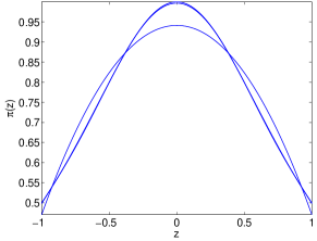
(a)

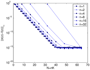
(b)

Figure 4.1. (A): Interpolants $\pi(z)$ to the Runge function $f(z)=1/(1+z^{2})$ with $K=4$ and $n=1,2,3$. (B): Dependence of interpolation error on the number of grid points $K$ for fixed number of derivatives $n$ at each grid point.

We now turn to the Runge function $f(z)=1/(1+z^{2})$, which is the subject of computations shown in Figure 4.1. A numerically stable method to calculate higher order derivatives of the Runge function for $z\in[-1,1]$ is implied by the following calculation:

$$f(z) = \frac{1}{2i}\left(\frac{1}{z-i}-\frac{1}{z+i}\right)$$

$$\frac{d^{r}f(z)}{dz^{r}} = (-1)^{r}\frac{r!}{2i}\left(\frac{1}{(z-i)^{r+1}}-\frac{1}{(z+i)^{r+1}}\right).$$

If $z-i=R\exp(i\theta)$, then we have $f^{(r)}(z)/r!=(-1)^{r-1}R^{r+1}\sin(r+1)\theta$. This formula has excellent numerical stability for $z\in[-1,1]$.

Figure 4.1 shows that the error in interpolating the Runge function is $c_{n}\exp(-\alpha nK)$. The positive constant $\alpha$ appears to be independent of $n$. However, $c_{n}$ increases with $n$. Therefore if we are allowed to use $N$ items of information about the function to form an accurate interpolant, the best choice for this example is to take them all to be function values.

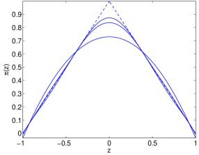
(a)

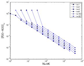
(b)

Figure 4.2. A): Interpolants $\pi(z)$ to the hat function $f(z)=1-|z|$ with $K=4$ and $n=1,2,3$. (B): Dependence of interpolation error on the number of grid points $K$ for fixed number of derivatives $n$ at each grid point.

For the hat function $f(z)=1-|z|$, Figure 4.2 shows that the error is proportional to $1/K$. If the error is represented in the form $c_{n}/nK$, $c_{n}$ once again increases with $n$.

The Runge function is analytic in an open set around $[-1,1]$, while the hat function is of bounded variation but not even continuously differentiable. In the case $n=1$, which corresponds to ordinary polynomial interpolation, the differing rates of convergence are easily explained by the difference in smoothness and analyticity [6]. That connection likely persists for $n>1$, which corresponds to Hermite interpolation.

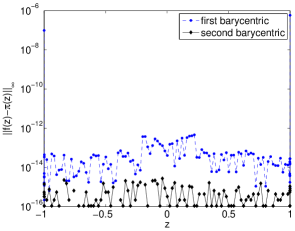
Figure 4.3. Interpolation errors to the Runge function $f(z)=1/(1+z^{2})$ with $K=512$ grid points and $n=48$ derivatives at each grid point. The first barycentric form is notably inaccurate at $z=\pm 1$.

The interpolations discussed so far used the second barycentric form. Figure 4.3 compares the first barycentric form (1.3) to the second (1.4). Even with $K=512$ grid points and $n=48$ derivatives there is no sign of numerical instability at all. The first barycentric form is less accurate but has small errors for $z\in(-1,1)$. At $z=\pm 1$, the first barycentric form produces much larger relative errors of about $10^{-7}$. It is well known that the Chebyshev polynomials are bounded by $1$ for $z\in[-1,1]$ but increase rapidly outside the interval. That phenomenon is magnified by several orders for the fundamental polynomials of Hermite interpolation. Thus we should expect the Hermite interpolant with $n=48$ to be very sensitive near the endpoints of the interval.

Another phenomenon noticeable from Figure 4.3 is that the errors are somewhat elevated near the center of the interval. The second barycentric form exhibits neither elevated error near the middle of the interval nor sensitivity at the end points. It has excellent numerical stability.

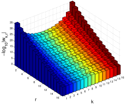
(a)

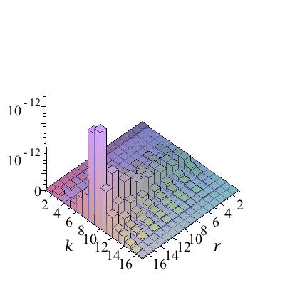
(b)

Figure 4.4. (A) Magnitude of the barycentric weights $w_{k,r}$ and (B) Relative error in the weights (the maximum relative error is $2.86\times 10^{-12}$. Both plots use $K=16$ grid points and $n=16$ derivatives at each grid point.

In Figure 4.4, we directly examine the weights used for barycentric interpolation. These weights are computed using Algorithm 1. Figure 4.4 uses $K=16$ and $n=16$. The Chebyshev points $z_{k}$ were multiplied by $2$ but the display in the figure does not use Leja ordering. From part (A) of the figure, we see that the weights $w_{k,r}$ are quite small especially when $r=0$. Thus in spite of using an interval of capacity $1$, the $C_{k}$ that occur on line 32 of Algorithm 1 are getting quite small. Using an interval of capacity $1$ still allows considerable fluctuations in $\prod_{k=1}^{K}(z-z_{k})$ around $1$ because it is only the $1/K$-th power which is guaranteed to converge to $1$. In computing the prefactor $C_{k}$, these fluctuations are raised to the power $n$, with $n$ being $16$ in this instance.

From part (B) of Figure 4.4, we see that the relative errors in the weights $w_{k,r}$ are quite small. However, the relative errors are the highest for $r=n$ and $z_{k}$ near the middle of the interval. These phenomena will be partially explained in the next section.

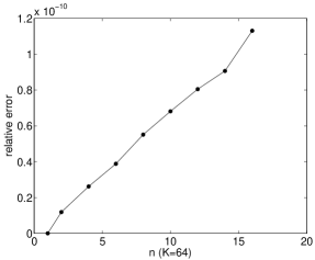
(a)

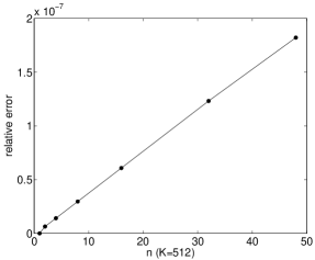
(b)

Figure 4.5. Maximum relative error in the barycentric weights $w_{k,r}$ as a function of the number of derivatives $n$ at each grid point.

In both Figures 4.4 and 4.5, the relative errors in the barycentric weights were obtained by comparing double precision results of a C++ program with extended precision computations in Maple. Figure 4.5 shows the increase in the maximum relative error in the barycentric weights $w_{k,r}$ with $n$, which is the number of derivatives used at each grid point. The increase is mild. Indeed, in part (B) of the figure, which uses $K=512$ the increase is only linear. Algorithm 1 for computing barycentric weights appears to have very good numerical stability.

5. Partial explanation of numerical stability

On line 32 of Algorithm 1, the weight $w_{k,r}$ is computed using $w_{k,r}=C_{k}\mathcal{I}_{r}$. The $C_{k}$ are merely products of differences and will be computed with excellent relative accuracy. We will restrict ourselves to the error accumulation in the computation of $\mathcal{I}_{r}$.

We assume that $\left\{\alpha_{1},\ldots,\alpha_{N}\right\}$ is a multiset of numbers and that $\mathcal{P}_{r}=\sum_{i=1}^{N}\alpha_{i}^{-r}$. The quantities $\mathcal{I}_{r}$ are defined by (2.4) and computed using $\mathcal{P}_{r}$ and the triangular identities of Lemma 2. For computing $w_{k,r}$, the multiset is taken to be $z_{1}-z_{k}$ repeated $n_{1}$ times, $z_{2}-z_{k}$ repeated $n_{2}$ times, and so on—see line 27 of Algorithm 1.

If $u$ is the unit round-off ($u=2^{-53}$ for IEEE double precision arithmetic), each arithmetic operation of the type $a+b$ will evaluate to $(a+b)(1+\delta)$ with $|\delta|<u$ in floating point arithmetic. If $1+\theta_{n}=\prod_{i=1}^{n}(1+\delta_{i})^{\rho_{i}}$, where $|\delta_{i}|\leq u$ and $\rho_{i}=\pm 1$, we have $\theta_{n}\leq\gamma_{n}$, where $\gamma_{n}$ is defined as $nu/(1-nu)$ (this is Lemma 3.1 of [8] for whose validity it is assumed that $nu<1$). This lemma is convenient for accumulating the effect of several rounding operations.

Another convenience is the counter notation [8, 15]. In this notation, $\left<n\right>$ stands for a product of the form $\prod_{i=1}^{n}(1+\delta_{i})^{\rho_{i}}$, where $|\delta_{i}|\leq u$ and $\rho_{i}=\pm 1$. Evidently, if $\left<n\right>=1+\delta$ then $|\delta|\leq\gamma_{n}$ (assuming $nu<1$). In floating point arithmetic, $(a+b)+c$ evaluates to $a\left<2\right>+b\left<2\right>+c\left<1\right>$.

If $\mathcal{P}_{1}=1/\alpha_{1}+\cdots+1/\alpha_{N}$ is computed in the order it is written, it evaluates to

$$1/\alpha_{1}\left<N\right>+1/\alpha_{2}\left<N\right>+1/\alpha_{3}\left<N-1\right>\cdots+1/\alpha_{N}\left<2\right>.$$

If $\alpha_{i}$ is perturbed to $\alpha_{i}\left<N-i+2\right>$, the computed result is the exact result. Thus the computation of $\mathcal{P}_{1}$ is backward stable. However, the computation of $\mathcal{P}_{1}$ can still have large relative errors if there are near cancellations. In Figure 4.5 (A), the relative error in $\mathcal{P}_{1}$ (the maximum over all $z_{k}$ which occurs for $z_{k}$ near the middle of the interval) is $1.18\times 10^{-11}$. In part (B), which correspond to $K=512$, the relative error in $\mathcal{P}_{1}$ is $6.42\times 10^{-9}$. If there is a point at $0$ and the positive and negative grid points are symmetric, the exact value of $\mathcal{P}_{r}$ is zero for $r$ an odd number and the relative error is infinite. However, in this case, $\mathcal{P}_{r}$ will have small relative error for even $r$ and the only power sums that influence the $\mathcal{I}_{r}$ correspond to even powers. If $r$ is even, $\mathcal{P}_{r}$ is always computed with excellent relative accuracy as there can be no cancellations.

Since the error analysis of $\mathcal{P}_{r}$ is relatively tractable and in view of the comments made in the previous paragraph, we will temporarily assume all the power sums $\mathcal{P}_{r}$ to be computed with small relative errors. The more complex issue is the manner in which the errors are amplified when the quantities $\mathcal{I}_{r}$ are computed using the triangular identities of Lemma 2. Figure 4.5 shows that the errors grow only very mildly when going from $\mathcal{P}_{r}$ to $\mathcal{I}_{r}$.

To understand the error growth, we recast the triangular identities of Lemma 2 into matrix form:

(5.1) $$\left(\begin{array}[]{ccccc}1\\ -\mathcal{P}_{1}&1\\ -\mathcal{P}_{2}&-\mathcal{P}_{1}&2\\ -\mathcal{P}_{3}&-\mathcal{P}_{2}&-\mathcal{P}_{1}&3\\ \ddots&\ddots&\ddots&\ddots&\ddots\end{array}\right)\left(\begin{array}[]{c}1\\ \mathcal{I}_{1}\\ \mathcal{I}_{2}\\ \mathcal{I}_{3}\\ \vdots\end{array}\right)=\left(\begin{array}[]{c}1\\ 0\\ 0\\ 0\\ \vdots\end{array}\right).$$

If the condition number of the matrix in (5.1) is $\kappa$, the norm-wise relative error in the $\mathcal{I}_{r}$ is bounded by $\frac{2\epsilon\kappa}{1-\epsilon\kappa}$, where $\epsilon$ is of the order of $u$, the unit round-off. Unfortunately, this bound is useless because $\kappa$ can be very large. If a single $\alpha_{i}$ is less than $1$, which is always the case, the $\mathcal{P}_{r}$ will increase exponentially with $r$. The condition number of the system (5.1), retaining only $n+1$ rows in that system, will increase exponentially with $n$.

Although $\kappa$ is quite bad, there is a simple way to get a matrix system equivalent to (5.1) with a small condition number. Suppose the $\alpha_{i}$s are all multiplied by a scaling factor $s$ and changed to $s\alpha_{i}$. Then $\mathcal{P}_{r}$ and $\mathcal{I}_{r}$ are transformed to $P_{r}=s^{-r}\mathcal{P}_{r}$ and $I_{r}=s^{-r}\mathcal{I}_{r}$, respectively. If $s$ is sufficiently large then $|P_{r}|\leq 1$ for $1\leq r\leq n$.

The $(n+1)\times(n+1)$ matrix obtained by replacing the power sums $\mathcal{P}_{r}$ by their scaled version $P_{r}$ has condition number bounded by $n+1$. In general, triangular systems have condition numbers that increase exponentially even if all the off-diagonal entries are bounded by $1$ in magnitude [19]. Here the situation is different because the diagonal entries increase in the order $1,1,2,3,\ldots$ We have the bound

$$|I_{r}|=\frac{|P_{r}+I_{1}P_{r-1}+\cdots+I_{r-1}P_{1}|}{r}\leq\frac{1+|I_{1}|+\cdots+|I_{r-1}|}{r}\leq 1,$$

where the last inequality is by induction. Thus all entries in the inverse will be bounded by $1$.

If a large scaling factor $s$ is used to control the condition number of the matrix, the difficulty comes in when we use $\mathcal{I}_{n}=s^{n}I_{n}$ to estimate the relative error in $\mathcal{I}_{n}$. The absolute errors in $I_{r}$ can be bounded by a quantity of the form $n^{5/2}u$, or even $nu$ if the scaling factor $s$ is chosen to make the power sums small enough , where $u$ is the unit round-off. However, if $I_{n}$ is much smaller than $1$ in magnitude, the norm-wise bounds will imply a large relative error in $I_{n}$ and in $\mathcal{I}_{n}$. This difficulty can be removed if a scaling factor $s$ can be found such that $|P_{r}|\leq 1$ for $1\leq r\leq n$ and $|I_{n}|$ is $\mathcal{O}(1)$. The linear growth in relative errors in Figure 4.5 suggests that such a scale might exist. Proving the existence of such a scale will require estimates of the quantities $\mathcal{P}_{r}$ and $\mathcal{I}_{r}$.

The discussion in this section partially backs up the finding of Figure 4.5 that the growth of relative errors in the barycentric weights with the order of the derivative is mild. The contribution to the errors made by $\mathcal{P}_{r}$ is therefore quite significant. Even though the computation of each power sum $\mathcal{P}_{r}$ is backward stable, the sum itself could be ill-conditioned. In fact, by looking up $n=1$ in Figure 4.5, we see that the relative error in $\mathcal{P}_{1}$ is not so small. We implemented compensated summation in x86 assembly language and verified that it does not reduce forward errors.

The following proposition allows us to verify the accuracy of some of the barycentric weights.

Proposition 3.

If the $\alpha_{i}$ are all positive, the relative error in $\mathcal{P}_{r}$ is bounded by $\gamma_{r+N}$ and the relative errors in $\mathcal{I}_{r}$ are bounded by $\gamma_{3rN}$ for sufficiently small unit round-off and $r\leq N$.

Proof.

The computed quantity $\mathcal{P}_{r}$ can be represented as

$$\alpha_{1}^{-r}\left<N+r\right>+\alpha_{2}^{-r}\left<N+r-1\right>+\cdots+\alpha_{N}^{-r}<r+1>.$$

Because each $\alpha_{i}$ is positive, the computed quantity can be represented as $\mathcal{P}_{r}\left<N+r\right>$ thus proving one half of the proposition.

For the other half, we note that that $\mathcal{I}_{r}=\left(\mathcal{P}_{r}+\mathcal{I}_{1}\mathcal{P}_{r-1}+\cdots+\mathcal{I}_{r-1}\mathcal{P}_{1}\right)/r$. By induction, the quantity computed for $\mathcal{I}_{r}$ can be represented as

$$\frac{\mathcal{P}_{r}\left<N+r\right>\left<r\right>+\cdots+\mathcal{I}_{r-1}\mathcal{P}_{1}\left<3(r-1)N\right>\left<N+1\right>\left<r\right>}{r}.$$

In this expression the $\left<r\right>$ factors that accompany each term in the numerator are caused by the arithmetic operations for computing $\mathcal{I}_{r}$ using $\mathcal{I}_{s}$ for $1\leq s\leq r-1$. The factors that accompany each term in the numerator can be multiplied and replaced by $\left<3Nr\right>$. Since each term is positive, it follows that the computed quantity can be represented as $\mathcal{I}_{r}\left<3Nr\right>$. ∎

This proposition implies that the weights $w_{k,r}$ are computed with excellent accuracy when $z_{k}$ is either the least or the greatest of the grid points. Indeed, we see from Figure 4.4(B) that the relative errors near the end points of the interval are very small. If $z_{k}$ is the least of the grid points, each $z_{j}^{\prime}$ , $1\leq j\leq K-1$ that occurs on line 27 of Algorithm 1 is negative and non-zero. Since $-1/z_{j}^{\prime}$ corresponds to $\alpha_{j}$ in Proposition 3, the proposition is immediately applicable. If $z_{k}$ is the greatest of the grid points, each $-1/z_{j}^{\prime}$ is negative and the proposition is not immediately applicable. However, it is evident from inspection that $\mathcal{P}_{r}$ and $\mathcal{I}_{r}$ are negative or positive according as $r$ is odd or even. Therefore every sum in the triangular identities of Lemma 2 has terms that are all positive or all negative. Thus the bounds on relative errors proved in the proposition will apply.

We have candidly highlighted the inadequacy, in situations not covered by Proposition 3, of the bounds that can be derived on the rounding errors in the computed barycentric weights. Thus the title of this section only claims a partial explanation. Existing results in rounding error analysis known to us give bounds which are highly pessimistic.

Numerical stability of barycentric Lagrange interpolation has been studied by Higham [9]. It may be suspected that the methods of that paper can be used for the numerical stability analysis of barycentric Hermite interpolation. However, that is far from being the case. The definition of the condition number used by Higham perturbs the function values but not the grid points. Such a definition is useful in the context of Lagrange interpolation because the Lagrange weights are obtained from products of the type $\prod_{j\neq k}(z_{j}-z_{k})$. The basic rules of double precision arithmetic imply right away that each Lagrange weight is computed with a very small relative forward error which can be easily bounded. In the case of Hermite interpolation, the computation of the weights is a great deal more complicated as we have emphasized. In particular, the computation involves back substitution or the inversion of the triangular system displayed explicitly in (5.1).

If good bounds on the forward errors of the barycentric weights $w_{k,r}$ can be obtained, the rounding error analysis simplifies greatly. The analysis of the first barycentric form (1.3) closely parallels the rounding error analysis of inner products of the type $\sum_{i=1}^{n}a_{i}b_{i}$. For the second barycentric form, one needs to tackle expressions of the form $A_{1}/A_{2}-A_{3}/A_{4}$, where each $A_{i}$ has the structure of an inner product. While this form is slightly more complicated algebraically, it poses none of the difficulties associated with triangular inversion or back substitution.

Higham’s treatise [8] on numerical algorithms discusses component-wise analysis of linear systems in Chapter 7 and triangular inversion in Chapter 8. We now explain why none of the results in those two chapters help explain the excellent numerical stability of barycentric Hermite interpolation illustrated in Figure 4.5. In the component-wise bound of Higham’s Theorem 7.4, it is crucial note the $|A^{-1}|$ that appears in the numerator. Viswanath and Trefethen have shown [19] that the inverses of triangular matrices generically have norms that are exponential in the dimension. Therefore such bounds are highly pessimistic for the situation illustrated in Figure 4.5. As we described in detail in the arguments leading up to Proposition 3, an attempt at mitigating the norm of the inverse by scaling the grid points is ultimately of no value. Exactly the same comments apply to Higham’s Lemma 7.9. The difficulty that one faces is more explicit in Higham’s Lemma 8.6, Theorem 8.7, and Theorem 8.14. In each of those results, the exponential dependence of the worst case bounds on the dimension of the matrix system is explicit. If those bounds are applied to (5.1), the resulting bounds on the errors in the barycentric weights, corresponding to the two plots in Figure 4.3, would be off by factors of $2^{64}$ and $2^{512}$, respectively.

The worst case bounds on rounding errors are exponential in the dimension of the linear system. The results of Viswanath and Trefethen [19] show that the same is true generically, thus suggesting strongly that the worst case bounds will be difficult to improve. It is noteworthy that Higham [8] begins the chapter on triangular systems by quoting authorities who realized decades ago that the bounds that can be derived on the error are usually pessimistic while in practice many triangular systems can be solved quite accurately.

We conclude by recommending the second barycentric form (1.4), with weights computed using the method of Butcher et al. [3] as presented in Algorithm 1, as the standard algorithm for Hermite interpolation. The reasons for this recommendation are the same as those given by Berrut and Trefethen [2] for barycentric Lagrange interpolation, namely, conceptual simplicity, excellent numerical stability, and flexibility in incorporating new data points. To those reasons, we may add the finding of Section 2 that barycentric Hermite interpolation has a lower operation count than Hermite interpolation using divided differences.

6. Acknowledgments

We thank Prof. Sergey Fomin for references that led us to attribute Lemma 2 to L. Crocchi [5, 1880].

References

- [1] J.-P. Berrut, R. Baltensperger, and H. Mittelmann. Recent developments in barycentric rational interpolation. In M.G. de Bruin, D.H. Mache, and J. Szabados, editors, Trends and Applications in Constructive Approximation, volume 151 of International Series of Numerical Mathematics, pages 27–51. Birkhäuser, 2005.
- [2] J.-P. Berrut and L.N. Trefethen. Barycentric Lagrange interpolation. SIAM Review, 46(3):501–517, 2004.
- [3] J.C. Butcher, R.M. Corless, L. Gonzalez-Vega, and A. Shakoori. Polynomial algebra for Birkhoff interpolants. Numerical Algorithms, 56:319–347, 2011.
- [4] S.D. Conte and C. de Boor. Elementary Numerical Analysis. McGraw-Hill Inc, 1980.
- [5] L. Crocchi. Una relazione fra le funzioni simmetriche semplici e le funzioni simmetriche complete. Giornale di Matematiche, XVIII:377–380, 1880.
- [6] P.J. Davis. Interpolation and Approximation. Dover Publications, 1975.
- [7] B. Fischer and L. Reichel. Newton interpolation in Fejér and Chebyshev points. Mathematics of Computation, 53(187):265–278, 1989.
- [8] N.J. Higham. Accuracy and Stability of Numerical Algorithms. Society for Industrial and Applied Mathematics, 2nd edition, 2002.
- [9] N.J. Higham. The numerical stability of barycentric Lagrange interpolation. IMA Journal of Numerical Analysis, 24(4):547, 2004.
- [10] L.M. Milne-Thomson. The Calculus of Finite Differences. Macmillan, 1933. Reprinted by Chelsea in 2000.
- [11] L. Reichel. Newton interpolation at Leja points. BIT Numerical Mathematics, 30:332–346, 1990.
- [12] B. Sadiq and D. Viswanath. Finite difference weights using the modified Lagrange interpolant. Arxiv preprint arXiv:1102.3203, 2011.
- [13] C. Schneider and W. Werner. Hermite interpolation: the barycentric approach. Computing, 46:35–51, 1991.
- [14] R.P. Stanley. Enumerative Combinatorics, volume 2. Cambridge, 1999.
- [15] G.W. Stewart. Introduction to Matrix Computations. Academic Press New York, 1973.
- [16] J. Szabados. On the order of magnitude of fundamental polynomials of Hermite interpolation. Acta Mathematica Hungarica, 61(3):357–368, 1993.
- [17] H. Tal-Ezer. High degree polynomial interpolation in Newton form. SIAM Journal on Scientific and Statistical Computing, 12:648–667, 1991.
- [18] K. Th. Vahlen. Rationale funktionen der wurzeln; symmetrische und affektfunktionen. Encyklopädie der Mathematischen Wissenschaften, 1:449–479, 1904.
- [19] D. Viswanath and L.N. Trefethen. Condition numbers of random triangular matrices. SIAM Journal on Scientific and Statistical Computing, 19:564–581, 1998.
- [20] W. Werner. Polynomial interpolation: Lagrange versus Newton. Math. Comp, 43:205–217, 1984.