The TreadmillSled of a curve
Abstract.
In [6], the author introduced the notion of TreadmillSled of a curve, which is an operator that takes regular curves in to curves in . This operator turned out to be very useful to describe helicoidal surfaces, for example, it provides an interpretation for the profile curve of helicoidal surfaces with constant mean curvature similar to the well known interpretation of the profile curve of Delaunay’s surfaces using conics, see [6]. In [4] the authors used the TreadmillSled to classify all helicoidal surfaces with constant anisotropic mean curvature coming from axially symmetric anisotropic energy density. Also, in [6], the author proves that an helicoidal surface different from a cylinder has constant Gauss curvature if and only if the TreadmillSled of its profile curve lies in a vertical semi line contained in the lower or upper half plane and not contained in the -axis… Why not the whole vertical line? and why the semi-line cannot be contained in the -axis? In this paper we provide several properties of the TreadmillSled operator, in particular we will answer the questions in the previous sentence. Finally, we prove that the TreadmillSled of the profile curve of a minimal helicoidal surface is either a hyperbola or a the -axis. The latter case occurs only when the surface is a helicoid.
2000 Mathematics Subject Classification:
53C42, 53A101. Introduction
The surface of revolution generated by the regular curve with is given by
The curve is called the profile curve. In [2], Delaunay proved that a surface of revolution has constant mean curvature if and only if it is a sphere, a cylinder or if its profile curve lies in the trace made by the focus of a conic, when this conic rolls along the -axis. When the conic used is a parabola, the surface is minimal and it is called catenoid; if the conic used is a hyperbola, the surface is called a nodoid and if the conic used is an ellipse, the surface is called an unduloid. Since an ellipse has two foci, the trace of each one of them generates an undoloid. It is not difficult to see that these two unduloids are essentially the same, one is a translation of the other. Figure 1.1 shows how the profile curve of an unduloid is constructed using an ellipe.
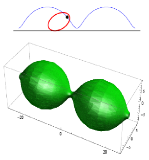
When we roll the parabola its focus traces a curve of infinity length. Figure 1.2 shows a catenoid and its profile curve.
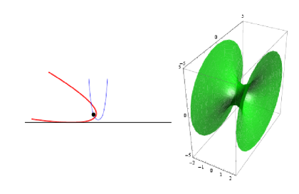
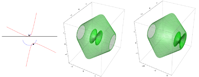
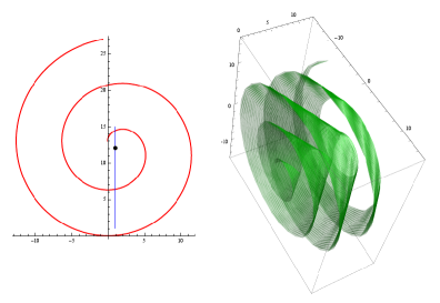
When we roll a set of hyperbolas, their foci trace two curves of finite length, each curve generates a cmc surface. It can be proven that we can translate one of these surfaces to obtain a smooth connected surface with constant mean curvature. If we repeat this connected piece over and over we obtain a complete cmc surface. In Figure 1.3 we show the trace of the foci, the two-piece cmc surface and the connected piece made by gluing the translation of one of the connected components of the initial two-piece surface to the other connected component.
Let us restate Delaunay’s theorem. Think of the operator that takes regular curves in into curves in given in the following way: For a regular curve , let denote the length of the curve from to and let us define
With this operator, Delaunay’s theorem implies that if is a piece of conic with focus at the origin, then is the profile curve of a surface of revolution with constant mean curvature. Notice how the center of the curve plays an important role in the definition of .
In [6], the author found a dynamical interpretation for helicoidal surfaces with constant mean curvature. For the sake of comparison, let us rewrite the first part of the introduction, but this time for helicoidal surfaces. The helicoidal surface generated by the regular curve is given by
The curve is called the profile curve. In [6], the author proved that a helicoidal surface has constant mean curvature one, if and only if, it is a cylinder of radius or if the origin of its profile curve, , trace the curve
| (1.1) |
when moves on a treadmill located at the origin aligned in the direction of the -axis. Figures 1.4 and 1.5 show examples of how the center of the profile curve generates curves of the form (1.1).
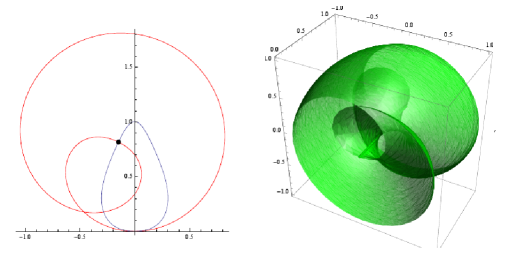
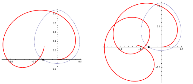
The fact that the TreadmillSled of the profile curve of a helicoidal surface with cmc is a closed curve allow us to define a fundamental piece of the profile curve, see Figure 1.5, which in turn, easily provides a dense versus properly-immersed duality property for all these cmc surfaces. See [6] for details.
Let us restate the previous theorem for helicoidal cmc surfaces. Think of the operator that take regular curves in into curves in given in the following way: for a regular curve , let us define
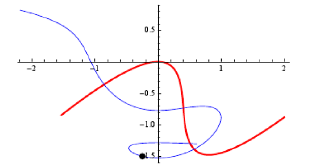
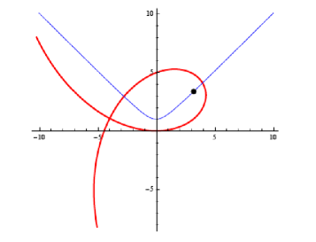
The letters stand for TreadmillSled Set. With this operator, we can say that if is the profile curve of a helicoidal surface with cmc one, then lies in a curve of the form (1.1). Notice how the center of curve plays an important role in the definition of . Figure 1.6 shows the TreadmillSled of the graph of a polynomial of degree 3.
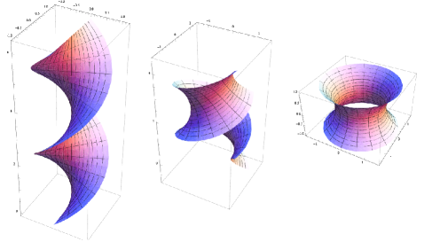
As more applications of the TreadmillSled, in [6], the author showed that a helicoidal surface has zero Gauss curvature if and only if the TreadmillSled of its profile curve lies in a vertical semi line contained in the upper or lower plane (see Figure 1.7).
Anytime we fixed a positive function on the Euclidean unit sphere we can define an anisotropic mean curvature for surfaces in . When is the constant function , the anisotropic mean curvature agrees with the mean curvature. Delaunay’s result for constant mean curvature of revolution was extended to anisotropic constant mean curvature surfaces of revolution by Miyuki and Palmer in 2008, [5]. Likewise, the dynamical interpretation for helicoidal constant mean curvature, [6], was extended to anisotropic constant mean curvature surfaces by Khuns and Palmer [4]. In the latter paper, Khuns and Palmer found a formula for the inverse of the operator TreadmillSled. Here in this paper we will elaborate more on this formula and prove some properties for the TreadmillSled. For purposes of a better understanding we will find an explicit parametrization for the TreadmillSled of a curve and we will be refereing to this parametrization of the TreadmillSled as just ; in this way, becomes an operator that takes a parametrized regular curve into a parametrized curve. We will show that this operator acts like the derivative operator for functions. For example,
-
•
Given , is an expression of and
-
•
If then and differ by a constant. This time the constant does not represent a translation on the graph like in the case of the derivative operator but it represents an oriented rotation that fixes the origin. More precisely, if we identify with the complex numbers, then for some constant .
-
•
When is in the image of the operator , there is a formula for that depends on , and only one antiderivative. The ambiguity of this antiderivative is responsible for the existence of the whole 1 parametric family of curves with the same TreadmillSled.
-
•
If we change the orientation of , that is, if we consider the curve , then .
If we look at figures 1.4, 1.5 and 1.6, we notice that the curves that are TreadmillSled have the property that their velocity vector is horizontal where the curve intercepts the axis. This is not a coincidence, actually we will show that a curve is the TreadmillSled of a regular curve if and only if
-
•
for some continuous function and
-
•
is a positive function.
From the first property we see that if , then and therefore the velocity vector is horizontal on points along the -axis. The second property is the reason why a whole vertical line cannot be the TreadmillSled of a regular curve. For a vertical line, always vanishes and therefore when the line touches the -axis, the function vanishes making the second property fail at this point. Also notice that if the vertical semi-line is contained in the -axis, then by the relation , we must have that vanishes and therefore reduces to just a point. It is easy to see that the TreadmillSled of a circle centered at the origin is just a point in the -axis. Notice that if the profile curve of a helicoidal surface is a circle centered at the origin then the surface is a cylinder.
At the end of this paper we prove that the TreadmillSled of the profile curve of a minimal helicoidal surface is either the -axis (when the surface is a helicoid), or it is a hyperbola centered at the origin.
2. The -TreadmillSled of a curve
In this paper we will assume that all functions have as many derivatives as needed. Let us start this section with a definition that extends the notion of TreadmillSled. One of the reasons we introduce this notion is because it provides an interpretation for the curve when , are curve in the complex plane with , see Corollary 2.9.
Definition 2.1.
Given a regular curve and a function , we define the -TreadmillSled of as the set of points
This set of points will be denoted by .
Remark 2.2.
Notice that the definition of the is independent of the parametrization, it only depends on the orientation of the curve. That is, if is a function with positive derivative and and , then
It is not difficult to see that the -TreadmillSled of can be viewed as the curve generated by doing the following steps:
-
•
Imagine that the curve is in a plane which can freely move. Moreover, let us assume that there is a hole in the origin of this plane and also let us assume that we have placed a pencil in this hole.
-
•
Imagine that another plane, this one fixed, contains a treadmill based at the origin with a device that allows the treadmill to incline at any angle.
-
•
The curve in the moving plane will generate another curve in the fixed plane, the -TreadmillSled of .
-
•
The -TreadmillSled of is the curve drawn on the fixed plane by the pencil located at the origin of the moving plane, when the curve passes on the treadmill with the property that, anytime the point is on the treadmill, the treadmill is aligned in the direction .
The following proposition will provide a formula to find the -TreadmillSled of a curve
Proposition 2.3.
Let be a regular curve in , if , then,
| (2.1) |
is a parametrization of the -TreadmillSled of . Here
and
Proof.
We will use the parameter to describe points in the set . For a fixed , let us find an oriented isometry of such that and . We know that
Notice that once we find , and , using the definition 2.1, we get that is a point in ; and therefore, when we vary in the interval , we obtain that is a parametrization of .
Since
We have that
and therefore,
Since , the last equation implies that , which implies that .
Now, using the equation we get that
Since , then the proposition follows.
∎
Remark 2.4.
The definition of TreadmillSled of a curve given in the introduction corresponds with the -TreadmillSled when is the zero function. Sometimes we will view not as a set but as the parametrized curve described in (2.1).
To be more precise, we will use Proposition 2.3 to define the TreamillSled as an operator that takes a regular parametric curve into a parametric curve.
Definition 2.5.
Let be a regular curve. We define the TreadmillSled of as the parametric curve given by
Corollary 2.6.
If we identify each point with the complex number , then
For any curve . Moreover, if the function is fixed, then, the -TreadmillSled of two curves is the same, if and only if the TreadmillSled of the curves is the same.
The following proposition gives us some insight about the nature of the operator -TreadmillSled defined in the set of regular curves. As we already notice, the -TreadmillSled of a curve is independent of the parametrization as long as the orientation is preserved. Therefore, there is not loss of generality if we assume that the curves in the domain of the operator -TreadmillSled are parametrized by arc-length.
Proposition 2.7.
Let and be two curves parametrized by arc-length. if and only if for some constant .
Proof.
Let and be functions such that . If , then
therefore, we may assume that . Using Proposition 2.3, we obtain that
Therefore, we have proven that if , then . Now let us assume that . Let us fix an such that . Since then . Let be a real number such that and let us consider . That is, , and moreover, we have that . Using Definition 2.5 we get that if is a curve parametrized by arc-length and , then,
For values of such that we get that
By the existence and uniqueness theorem of ordinary differential equations we get that the conditions and imply that for all near . Since both curves are regular, by a continuity argument we conclude that the real number is independent of and therefore for all . We then get for some . This finishes the proof of the proposition.
∎
Remark 2.8.
Let us define . If is an arc-length parametrized curve and , then,
With this definition of we have that the curvature of is . Notice that if , then . Therefore, if we know the curvature of a curve parametrized by arc-Length and a given angle for the velocity vector, let’s say , then
The following corollary provides a way to program the inclination on a treadmill (find the function ) if we want to get the curve as the -TreadmillSled of .
Corollary 2.9.
If is a regular curve with curvature function and is a function, then
where and
We will now characterize the range of the operator TreadmillSled and find an inverse of this operator. Under the assumption that a curve is in the range of the operator , the formula for the inverse of the TreadmillSled provided below was found in [4].
Proposition 2.10.
Let us denote . is the Treadmillsled of a regular curve if and only if for some continuous function and . More precisely, if and satisfy the two previous conditions, and is an antiderivative of , then,
Proof.
Let us assume that is the TreadmillSled of a curve . Let us first consider the case when is parametrized by arc-Length. If we denote by the curvature of , then, using Remark 2.8 we obtain,
Therefore,
and
Taking we conclude that and . If we now consider a regular curve , then we have that where is parametrized by arc-length and is a function with . Therefore, by either Remark 2.2 or by Definition 2.5, we get that if is the TreadmillSled of , then where is the TreadmillSled of . Since is parametrized by arc-length, then is continuous and . Therefore, is continuous and
This inequality finishes the proof of one of the implications of the Proposition. Let us assume now that the functions are given and that is continuous and that . We need to prove that if then
satisfies that . Using the fact that
we get that
Therefore,
Since , we get,
Since we have that , then we conclude that and therefore is a regular curve.
Since,
and,
we conclude that . This completes the proof of the proposition.
∎
3. A dynamical interpretation for helicoidal minimal surfaces
Helicoidal minimal hypersurfaces have been understood for a long time. For a detailed study we refer to the last section of the last chapter of the book of Differential Geometry by Graustein [3]. We have that all the isometry surfaces (except for the catenoid) from the well known family of surfaces that starts with a helicoid and ends with a catenoid are helicoidal minimal surfaces. Actually, every helicoidal minimal surface belongs to one of these families.
A similar result for helicoidal cmc surfaces was proven in [1] by Do Carmo and Dajczer. They proved that every helicoidal surface belongs to a family of isometry surfaces that continuously move from an unduloid to a nodoid. In this section we provide a dynamical interpretation for the profile curve of a helicoidal minimal surface. Let us state and prove the main theorem in this section.
Theorem 3.1.
A complete helicoidal surface is minimal if and only if the TreamillSled of its profile either is the -axis and is a helicoid or it is one of the branches of the hyperbola for some non zero .
Proof.
Let us assume that the profile curve is parametrized by arc-length. If then by Definition 2.5 we have
Since we are assuming that is parametrized by arc-length, there exists a function such that . From the previous equation we get that
We this definition of and the definition of the function and given above, we obtain that
A direct computation shows that
is a Gauss map of the immersion and, with respect to this Gauss map, the first and second fundamental form are given by
Using the values above we get that the mean curvature of the is given by
Therefore, the equation , that is, the minimality of the immersion , implies
From the definition of and we get that
Likewise we obtain that . Therefore if is minimal, replacing the expression for above, we get that
A direct verification shows that if satisfies the differential equation above then,
If then and . That is, in this case the TreadmillSled of is the -axis. A direct computation using the inverse formula for the TreadmillSled, see Proposition 2.10, gives us that is a line through the origin, and therefore is a helicoid. If is not zero, we get by squaring the centered equation above, that the TreadmillSled lies in one of the branches of the hyperbola . A direct computation shows that if we parametrize one of these branches with the right orientation, that is, making sure that the second condition of Proposition 2.10 holds true, then we will find a parametrization of a profile curve that produces a minimal helicoidal surface. This finish the proof of the theorem.
∎
References
- [1] Dajczer, M., Do Carmo, M. Helicoidal surfaces with constant mean curvature, Tohoku
- [2] Delaunay, C. Sur la surface de revolution dont la courbure moyenne est constante, J. Math. Pures Appl., Ser. 1 6, (1841), 309-320.
- [3] Graustein, W. Differential Geometry, New York, The Macmillan Company, 1935.
- [4] Kuhns, C. and Palmer, B. Helicoidal surfaces with constant anisotropic mean curvature, arXiv:1010.1557
- [5] Miyuki, K. and Palmer, B. Rolling construction for anisotropic Delaunay surfaces. Pacific J. Math. 234 (2008), no. 2, 345-378.
- [6] Perdomo, O. A dynamical interpretation of the profile curve of cmc Twizzlers surfaces, arXiv:1001.5198