B.P. 6759, F-45067 ORLÉANS Cedex 2.
Computing in the fractal cloud:
modular generic solvers for
SAT and Q-SAT variants
Abstract
Abstract geometrical computation can solve hard combinatorial problems efficiently: we showed previously how Q-SAT can be solved in bounded space and time using instance-specific signal machines and fractal parallelization. In this article, we propose an approach for constructing a particular generic machine for the same task. This machine deploies the Map/Reduce paradigm over a fractal structure. Moreover our approach is modular: the machine is constructed by combining modules. In this manner, we can easily create generic machines for solving satifiability variants, such as SAT, #SAT, MAX-SAT.
Keywords.
Abstract geometrical computation; Signal machine; Fractal; SAT; Massive parallelism; Model of computation.
1 Introduction
Since their first formulations in the seventies, problems of Boolean satisfiability have been studied extensively in the field of computational complexity. Indeed, the most important complexity classes can be characterized — in terms of reducibility and completeness — by such problems e.g. SAT for NP (Cook, 1971) and Q-SAT for PSPACE (Stockmeyer and Meyer, 1973). As such, it is a natural challenge to consider how to solve these problems when investigating new computing machinery (quantum, NDA, membrane, hyperbolic spaces…) (Păun, 2001; Margenstern and Morita, 2001; Alhazov and Pérez-Jiménez, 2007).
This is the line of investigation that we have been following with signal machines (Durand-Lose, 2005), an abstract and geometrical model of computation. We showed previously how such machines were able to solve SAT (Duchier et al., 2010a) and Q-SAT (Duchier et al., 2010b) in bounded space and time. But in both cases, the machines were instance-specific i.e. depended on the formula whose satifiability was to be determined. The primary contribution of the present paper is to exhibit a particular generic signal machine for the same task: it takes the instance formula as an input encoded (in polynomial-time by a Turing machine) in an initial configuration. We further improve our previous results by describing a modular approach that allows us to easily construct generic machines for other variants of SAT, such as #SAT or MAX-SAT.
The model of signal machines, called abstract geometrical computation, involves two types of fundamental objects: dimensionless particles and collision rules. We use here one-dimensional machines: the space is the Euclidean real line, on which the particles move with a constant speed. Collision rules describe what happens when several particles collide. By representing the continuous time on a vertical axis, we obtain two-dimensional space-time diagram, in which the motion of the particles are materialized by segment lines called signals.
Signal machines can simulate Turing machines, and are thus Turing-universal (Durand-Lose, 2005). They are also capable of analog computation by using the continuity of space and time to simulate analog models such as BSS’s one (Durand-Lose, 2008; Blum et al., 1989) or computable analysis (Durand-Lose, 2009). Other geometrical models of computation exist: colored universes (Jacopini and Sontacchi, 1990), geometric machines (Huckenbeck, 1989), piece-wise constant derivative systems (Bournez, 1997), optical machines (Naughton and Woods, 2001)…All these models, including signal machines, belong to a larger class of models of computation, called unconventional, which are more powerful than classical ones (Turing machines, RAM, -calculus …). Among all these abstract models, the model of signal machines distinguishes itself by realistic assumptions respecting the major principles of physics — finite density of information, respect of causality and bounded speed of information — which are, in general, not respected all at the same time by other models. Nevertheless, signal machines remain an abstract model, with no a priori ambition to be physically realizable, and is studied for theoretical issues of computer sciences.
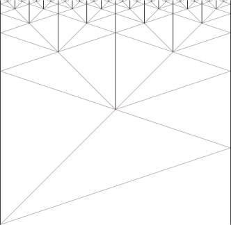
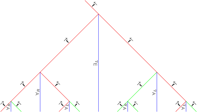
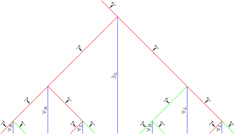
As signal machines take their origins in the world of cellular automa (as illustrated in Fig. 1), they can also be viewed as a massively parallel computational device. This is the approach proposed here: we put in place a fractal compute grid, then use the Map/Reduce paradigm to distribute the computations, then aggregate the results.
The Map/Reduce pattern, pioneered by Lisp, is now standard in functional programming: a function is applied to many inputs (map), then the results are aggregated (reduce). Google extended this pattern to allow its distributed computation over a grid of possibly a thousand nodes (Dean et al., 2004). The idea is to partition the input (petabytes of data) into chunks, and to process these chunks in parallel on the available nodes.
When solving combinatorial problems, we are also faced with massive inputs; namely, the exponential number of candidate solutions. Our approach is to distribute the candidates, and thus the computation, over an unbounded fractal grid. In this way, we adapt the map/reduce pattern for use over a grid with fractal geometry.
Our contribution in this paper is three fold: first, we show how Q-SAT can be solved in bounded space and time using a generic machine, where the input (the formula) is simply compiled into an initial configuration. This improves on our previous result where the machine itself depended on the formula. Second, we propose the first architecture for fractally distributed computing (the fractal cloud) and give a way to automatically shrink the data into this structure by means of a lens device. Third, we show how generic machines for many variants of SAT can be assembled by composing independent modules, which naturally emerged from the generalization of our previous family of machines into a single machine solving Q-SAT. Each module can be programmed and understood independently.
The paper is structured as follow. Signal machines are introduced in Section 2. Section 3 presents the fractal tree structure used to achieve massive parallelism and how general computations can be inserted in the tree. Section 4 details this implementation for a Q-SAT solver and Section 5 explains how some variants of satisfiability problems can be solved with the same approach. Complexities are discussed in Section 6 and conclusions and remarks are gathered in Section 7.
2 Definitions
Signal machines are an extension of cellular automata from discrete time and space to continuous time and space. Dimensionless signals/particles move along the real line and rules describe what happens when they collide.
Signals.
Each signal is an instance of a meta-signal. The associated meta-signal defines its velocity and what happen when signals meet. Figure 2 presents a very simple space-time diagram. Time is increasing upwards and the meta-signals are indicated as labels on the signals.
| Meta-signal | Speed |
|---|---|
| 0 | |
| 1 | |
| 3 | |
|
||||||
|
||||||
Generally, we use over-line arrows to indicate the direction and speed of propagation of a meta-signal. For example, and denotes two different meta-signals; the first travels to the right at speed 1, while the other travels to the left at speed . w and a are both stationary meta-signals.
Collision rules.
When a set of signals collide, they are replaced by a new set of signals according to a matching collision rule. A rule has the form:
where all are meta-signals of distinct speeds as well as (two signals cannot collide if they have the same speed and outcoming signals must have different speeds). A rule matches a set of colliding signals if its left-hand side is equal to the set of their meta-signals. By default, if there is no exactly matching rule for a collision, the behavior is defined to regenerate exactly the same meta-signals. In such a case, the collision is called blank. Collision rules can be deduced from space-time diagrams as on Fig. 2. They are also listed on the right of this figure.
Signal machine.
A signal machine is defined by a set of meta-signals, a set of collision rules, and and initial configuration, i.e. a set of particles placed on the real line. The evolution of a signal machine can be represented geometrically as a space-time diagram: space is always represented horizontally, and time vertically, growing upwards. The geometrical algorithm displayed in Fig. 2 computes the middle: the new a is located exactly halfway between the initial two w.
3 Computing in the fractal cloud
Constructing the fractal:
the fractal structure that interests us is based on the simple idea of computing the middle illustated in Figure 2. We just indefinitely repeat this geometrical construction: once space has been halved, we recursively halve the two halves, and so on.
This is illustrated in Figure 3(a), and can be generated by the following rules:111For brevity, we will always omit the rules which can be obtained from the others by symmetry. We refer to Appendix 0.A for more details.
using as the initial configuration. This produces a stack of levels: each level is half the height of the previous one. As a consequence, the full fractal has width 1 and height 1.
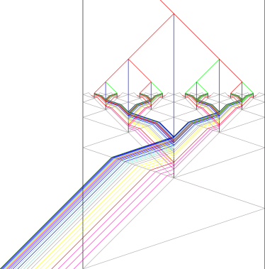
Distributing a computation:
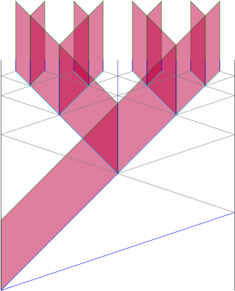
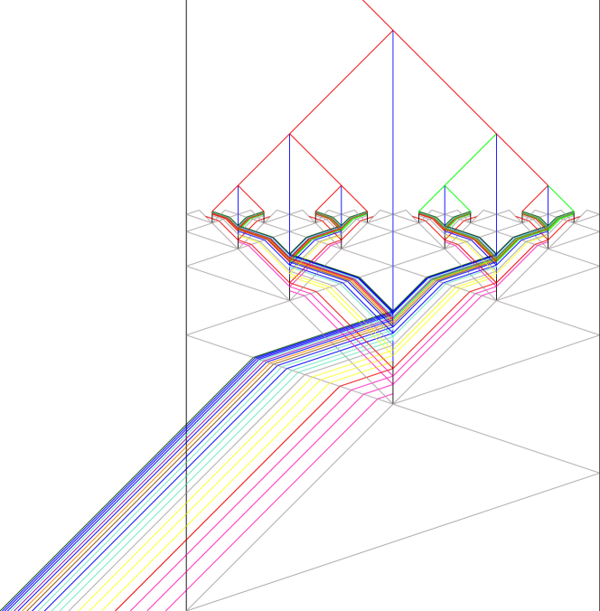
the point of the fractal is to recursively halve space. At each point where space is halved, we position a stationary signal (a vertical line in the space-time diagram). We can use this structure, so that, at each halving point (stationary signal), we split the computation in two: send it to the left with half the data, and also to the right with the other half of the data.
The intuition is that the computation is represented by a beam of signals, and that stationary signals split this beam in two, resulting in one beam that goes through, and one beam that is reflected.
Unfortunately, a beam of constant width will not do: eventually it becomes too large for the height of the level. This can be clearly seen in Figure 3(b).
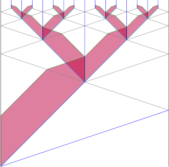
The lens device:
the lens device narrows the beam by a factor of 2 at each level, thus automatically adjusting it to fit the fractal. It is implemented by the following meta-rule: unless otherwise specified, any signal is accelerated by and decelerated and split by any stationary signal s.
Generic computing over the fractal cloud:
with the lens device in effect, generic computations can take place over the fractal by propagating a beam from an initial configuration. We write for an initial configuration with a sequence of signals. Geometrically, it can be seen easily that, in order for the beam to fit through the first level, the sequence must be placed in the interval .
Stopping the fractal:
For finite computations, we don’t need the entire fractal. The module can be inserted in the initial configuration to cut the fractal after levels have been generated.
The subbeam are the inhibitors for . One inhibitor is consumed at each level, after which takes effect and turns into , then crosses a and turns on the other side into . Finally the annihilation rule brings the fractal to a stop. Thus, a computation uses only levels. It can be seen geometrically that, for the collision of with to occur before the latter meets with , must initially be placed in .
4 A modular Q-SAT solver
Q-SAT is the satisfiability problem for quantified Boolean formulae (QBF). A QBF is a closed formula of the form:
where and is a quantifier-free formula of propositional logic. A recursive algorithm for solving Q-SAT is:
where is a ground Boolean formula. This is exactly the structure of our construction: each quantified variable splits the computation in 2, is sent to the left and to the right, and subsequently the recursively computed results that come back are combined (with for and for ) to yield the result for the quantified formula. This process can be viewed as an instance of Map/Reduce, where the Map phase distributes the combinatorial exploration of all possible valuations across space using a binary decision tree, and the Reduce phase collects the results and aggregates them using quantifier-appropriate Boolean operations. Our Q-SAT solver is modularly composed as follows:
We describe the modules decide, map:sat, and reduce:qsat below.
4.1 Setting up the decision tree
For a QBF with variables, we need 1 level per variable, and then at level we have a ground propositional formula that needs to be evaluated. Thus, the first module we insert is to create levels. We then insert because we want to use the first levels as decision points for each variable.
4.2 Compiling the formula
The intuition is that we want to compile the formula into a form of inverse polish notation to obtain executable code using postfix operators. At level all variables have been decided, and have become or . The ground formula, regarded as an expression tree, can be executed bottom up to compute its truth value: the resulting signal for a subexpression is sent to interact with its parent operator.
The formula is represented by a beam of signals: each subformula is represented by a (contiguous) subbeam. A subformula that arrives at level starts evaluating when it hits the stationary a. When its truth value has been computed, it is reflected so that it may eventually collide with the incoming signal of its parent connective.
Compilation.
For binary connectives: one argument arrives first, it is evaluated, and its truth value is reflected toward the incoming connective; but, in order to reach it, it must cross the incoming beam for the other argument and not interact with the connectives contained therein. For this reason, with each subexpression, we associate a beam of inhibitors that prevents its resulting truth value to interact with the first connectives that it crosses. We write for the compilation of into a contribution to the initial configuration, and for the number of occurrences of connectives in .
Variables.
We want variable to be decided at level . This can be achieved using inhibitors.
For variable , the idea is to protect from being assigned into and until it reaches the level. This is achieved with a stack of signals : at each level, the first turns the stationary signal x into (the non-assigning version of x), and dies. The following are simply split, and so is but it additionally turns back into x. After the first levels, all the have been consumed so that finally collides with x and splits into going left and going right.
Evaluation.
When hitting a at level , is reflected as , and as : these are their activated versions which can interact with incoming connectives to compute the truth value of the formula according to the rules below (for ; other connectives are similar, cf Appendix 0.A). See Fig. 5(a) for an example.
Initial configuration
Storing the result.
In order to make the result easily exploitable by the Reduce phase, we now store it as the stationary signal at level ; it replaces a.
The complete Map phase in implemented by:
4.3 Aggregating the results
As explained earlier, the results for an existentially (resp. universally) quantified variable must be combined using (resp. ).
Setting up the quantifiers.
We turn the decision points of the first levels into quantifier signals. Moreover, at each level, we must also take note of the direction in which the aggregated result must be sent. Thus represents an existential quantifier that must send its result to the left.
Aggregating the results.
Actual aggregation is initiated by and then executes according to the rules given in Fig 5(b).
The complete Reduce phase
is implemented by
5 Machines for SAT variants
Similar machines for variants of SAT can be obtained easily, typically by using different modules for the Reduce phase.
ENUM-SAT.
returning all the satisfying assignments for a propositional formula can be achieved easily by storing them as stationary beams.
#SAT.
counting the number of satisfying assignments for can be achieved using signals for a binary adder. For lack of space, we cannot exhibit the rules here, but they can be found in Appendix 0.B.
MAX-SAT.
finding the maximum number of clauses that can be satisfied by an assignment. Here we must count the number of satisfied clauses rather than the number of satisfying assignments, and then stack a module for computing the max of two binary numbers.
6 Complexities
As mentioned in Sect. 1, we implement algorithms for satisfiability problems on signal machines in order to investigate the computational power of our abstract geometrical model of computation and to compare it to others. As we shall see, for such comparisons to be meaningful, the way complexity is measured must be adapted to the nature on the computing machine.
Since signal machines can be regarded as the extension of cellular automata from discrete to continous time and space, it might seem natural to measure the time (resp. space) complexity of a computation using the height (resp. width) of its space-time diagram. But, in our applications to SAT variants, these are bounded and independant of the formula: the Map phase is bounded by the fractal, and, by symmetry, so is the Reduce phase. Indeed, in general, by an appropriate scaling of the initial configuration, a finite computation could be made as small as desired. Thus, height and width are no longer pertinent measures of complexity.
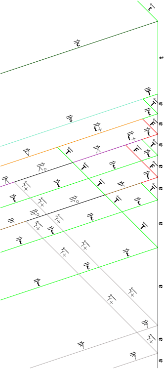
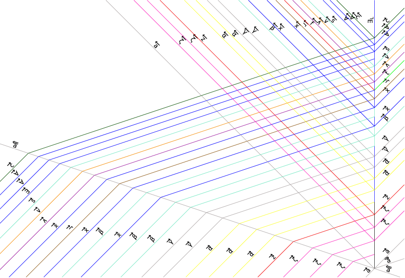
Instead, we should regard our construction as a massively parallel computational device transforming inputs into outputs. The input is the initial configuration at the bottom of the diagram, and the output is the truth value signal coming out at the top, as seen in Fig. 6 for formula . The transformation is performed in parallel by many threads: a thread here is an ascending path through the diagram from an input to the output, and the operations executed by the thread are the collisions occurring on this path.
Formally, we view a space-time diagram as a directed acyclic graph of collisions (vertices) and signals (arcs) oriented according to causality. Time complexity is then defined as the maximal size of a chain of collisions i.e. the length of the longest path, and space complexity as the maximal size of an anti-chain i.e. the size of the maximal set of signals pairwise un-related. This model-specific measure of time complexity is called collisions depth.
For the present construction, if is the size of the formula and the number of variables, space complexity is exponential: during evaluation, independent computations are executed in parallel, each one involving approximately signals, so that the total space complexity is in .
Regarding the time complexity: for each subformula, the compilation process introduces a number of signals at most linear in . Thus the number of signals in the initial configuration is . The primary contribution to the number of collisions along an ascending path comes, at each of the levels, from the reflected beam crossing the incoming beam. Thus a thread involves collisions, making the collision depth cubic in the size of the formula instead of quadratic for our previous family of machines, giving us an idea of the price for genericity.
7 Conclusion
We showed in this paper that abstract geometrical computation can solve Q-SAT in bounded space and time by means of a single generic signal machine. This is achieved through massive parallelism enabled by a fractal construction that we call the fractal cloud. We adapted the Map/Reduce paradigm to this fractal cloud, and described a modular programming approach making it easy to assemble generic machines for SAT variants such as #SAT or MAX-SAT.
As we explained in Sect. 6, time and space are no longer appropriate measures of complexity for geometrical computations. This leads us to propose new definitions of complexity, specific to signal machines, and taking in account the parallelism of the model: time and space complexities are now defined respectively by the maximal sizes of a chain and an anti-chain, when the diagram is regarded as a directed acyclic graph. Time complexity thus defined is called collision depth. According to these new definitions, our construction has exponential space complexity and cubic time complexity.
Although the model is purely theoretical and has no ambition to be physically realizable, it is a significant and distinguishing aspect of signal machines that they solve satifiability problems while adhering to major principles of modern physics — finite density and speed of information, causality — that are typically not considered by other unconventional models of computation. They do not, however, respect the quantization hypothesis, nor the uncertainty principle.
We are know furthering our research along two axes. First, the design and applications of other fractal structures for modular programming with fractal parallelism. Second, the investigation of computational complexity classes, both classical and model-specific for abstract geometrical computation.
References
- Alhazov and Pérez-Jiménez [2007] Artiom Alhazov and Mario J. Pérez-Jiménez. Uniform solution of Q-SAT using polarizationless active membranes. In J. Durand-Lose and M. Margenstern, editors, 5th International Conference on Machines, Computations, and Universality (MCU ’07), number 4664 in LNCS, pages 122–133. Springer, 2007.
- Blum et al. [1989] L. Blum, M. Shub, and S. Smale. On a theory of computation and complexity over the real numbers: NP-completeness, recursive functions and universal machines. Bulletin of the American Mathematical Society, 21(1):1–46, 1989.
- Bournez [1997] Olivier Bournez. Some bounds on the computational power of piecewise constant derivative systems. In ICALP ’97, number 1256 in LNCS, pages 143–153, 1997.
- Cook [1971] Stephen A. Cook. The complexity of theorem proving procedures. In 3rd Symposium on Theory of Computing (STOC ’71), pages 151–158. ACM, 1971.
- Dean et al. [2004] Jeffrey Dean, Sanjay Ghemawat, and Google Inc. Mapreduce: simplified data processing on large clusters. In Proceedings of the 6th Conference on Symposium on Opearting Systems Design & Implementation (OSDI’ 04). USENIX Association, 2004.
- Duchier et al. [2010a] Denys Duchier, Jérôme Durand-Lose, and Maxime Senot. Fractal parallelism: Solving SAT in bounded space and time. In O. Cheong, K-Y. Chwa, and K. Park, editors, 21st International Symposium on Algorithms and Computation (ISAAC ’10), number 6506 in LNCS, pages 279–290. Springer, 2010a.
- Duchier et al. [2010b] Denys Duchier, Jérôme Durand-Lose, and Maxime Senot. Massively parallel automata in Euclidean space-time. In J. Beal, O. Michel, and A. Spicher, editors, 3rd International Spatial Computing Workshop (SCW ’10)(extended abstracts of unpublished papers), 2010b. URL http://www.spatial-computing.org.
- Durand-Lose [2005] Jérôme Durand-Lose. Abstract geometrical computation: Turing computing ability and undecidability. In B.S. Cooper, B. Löwe, and L. Torenvliet, editors, New Computational Paradigms, 1st Conf. Computability in Europe (CiE ’05), number 3526 in LNCS, pages 106–116. Springer, 2005.
- Durand-Lose [2008] Jérôme Durand-Lose. Abstract geometrical computation with accumulations: Beyond the Blum, Shub and Smale model. In Arnold Beckmann, Costas Dimitracopoulos, and Benedikt Löwe, editors, Logic and Theory of Algorithms, 4th Conf. Computability in Europe (CiE ’08) (abstracts and extended abstracts of unpublished papers), pages 107–116. University of Athens, 2008.
- Durand-Lose [2009] Jérôme Durand-Lose. Abstract geometrical computation and computable analysis. In J.F. Costa and N. Dershowitz, editors, International Conference on Unconventional Computation 2009 (UC ’09), number 5715 in LNCS, pages 158–167. Springer, 2009.
- Huckenbeck [1989] Ulrich Huckenbeck. Euclidian geometry in terms of automata theory. Theoret. Comp. Sci., 68(1):71–87, 1989.
- Jacopini and Sontacchi [1990] Giuseppe Jacopini and Giovanna Sontacchi. Reversible parallel computation: an evolving space-model. Theoret. Comp. Sci., 73(1):1–46, 1990.
- Margenstern and Morita [2001] Maurice Margenstern and Kenichi Morita. NP problems are tractable in the space of cellular automata in the hyperbolic plane. Theor. Comp. Sci., 259(1-2):99–128, 2001.
- Naughton and Woods [2001] Thomas J. Naughton and Damien Woods. On the computational power of a continuous-space optical model of computation. In M. Margenstern, editor, Machines, Computations, and Universality (MCU ’01), number 2055 in LNCS, pages 288–299, 2001.
- Păun [2001] Gheorghe Păun. P-systems with active membranes: Attacking NP-Complete problems. Journal of Automata, Languages and Combinatorics, 6(1):75–90, 2001.
- Stockmeyer and Meyer [1973] Larry J. Stockmeyer and Albert R. Meyer. Word problems requiring exponential time. In 5th ACM Symposium on Theory of Computing (STOC ’73), volume 16, pages 1–9, 1973.
Appendix 0.A Details of the modules
In the following, we generally define the collision rules only for one side, as the corresponding rules for the other side can be deduced by symetry. We give here the rules for all modules: first the modules for building and stopping the fractal tree, then the modules for setting and using the tree for satisfiability problems and finally the modules specific to each variants of SAT.
All the diagrams of the paper were generated by Durand-Lose’s software, implemented in Java, and corresponds to a run of our Q-SAT solver for the formula:
0.A.1 The fractal cloud
Constructing the fractal:
The following rules on the left correspond to the bounce of and
on the wall w. Rules on the right are the step of induction
for starting the next level: the initial signals and are
duplicated on the right and the left, and the stationary signal a is created
exactly at the middle of the previous stage. The result is given by Fig. 7.

Stopping the fractal:
The role of this module is to stop the fractal after levels — levels for assigning the variables and level for the evaluation of the ground formula. For this, we use a stack of signals and one signal . The signals are used both as a counter, one signal being killed at each level, and as inhibitors to the effect of . After levels, only remains and can stop the construction of the fractal at level . Here are the corresponding rules:
The lens effect:
The general idea is that any signal is accelerated by and decelerated and split by any stationary signal s. There are some special cases to handle for the deceleration and the split, some particular signals being stopped at this moment. But in all cases, signals are always accelerated by . Figure 8 zooms on a split and illustrates the lens effect on the beam as well as the assignment of the top-most .
General case: for any stationary signal s (more exactly, s is either a, , x, , , , or ) and for any signal distinct of and , we have:
Case of and : the rules for applying the lens effect to and are given previously in §.Stopping the fractal. The stationary signal involved here is a, which kills the first , becomes and splits and decelerates the next signals and , and then becomes a again.
Case of : the first is stopped by the stationary signal a, which becomes x and decelerates and splits the next coming .
Case of quantifiers signals: the first quantifier signal, or , colliding with a stationary x is stopped and turns x into or (). This is achieved by the rules:
The next quantifier signals are decelerated and split by the new stationary signal or . In the following rules, we have :
0.A.2 The tree for satisfiabilty problems
Activation of the decision tree:
Representation of a variable:
As we explained in the paper, the variable is represented by a stack of signals: one signal and signals . The role of the signals is to protect from being assigned before the level. The first signal of the stack is stopped at the next split, so that signals have disappeared just before the stage. This is illustrated in Fig. 8 and modelised by the following rules:
Compilation of the formula:
We propose here a recursive algorithm which takes as input an unquantified formula — a SAT-formula — and outputs the part of the initial configuration corresponding to the formula. In the following schemes of compilation, designates the number of occurences of Boolean connectives in formula .
Evaluation:
The rules for the evaluation follow the classical Boolean operations. We explained earlier that some inhibiting signals — the — are needed to allow the result of the first evaluated argument of a binary connective to traverse the beam of the other, as yet unevaluated, argument without reacting with the connectives contained therein, and only interact with its actual syntactical parent connective. Figure 9 displays the evaluation of the formula for the case .
Storing the results:
Appendix 0.B Modularity and satifiability variants
0.B.1 Q-SAT
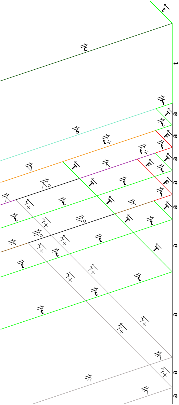
To proceed to the aggregation process, we join the results coming from right and left two-by-two. This is done with a stationary signal indicating the type of operation to perform — a conjunction for and a disjunction for — and the direction of the resulting signal — left or right. The whole process is displayed in Fig. 10.
Setting up the reduce stage:
Executing the reduce stage:
Initiation:
Performing the disjunction:
Performing the conjunction:
Putting all the modules together, we obtain for the running example the initial configuration shown by Fig. 11.
The global construction is displayed by Fig. 12

0.B.2 #SAT
#SAT is the problem of counting the number of solutions of SAT. We recall that this problem is complete for the class #P i.e. the class of NP-problems for which their solutions can be counted is polynomial time.
To solve #SAT, as a SAT-formula is a special instance of a Q-SAT formula in which all quantifiers are existential, we can use our Q-SAT solver and we add a special module for counting the truth evalution of the formula during the aggregation process. The counting is performed by a binary adder.
Setting up the reduce stage:
Executing the reduce stage:
Rules for the binary adder (for the subscript, the rules for the are similar, but with the output going to the left):
0.B.3 ENUM-SAT
ENUM-SAT is the problem of enumerating all the solutions for an instance of SAT: we want to know all the truth assignements of variables for which the formula is satisfiable. We can also consider a particular case of ENUM-SAT: the problem ONESOL-SAT, which consists in returning only one valuation satifying the formula, when the formula is satisfiable.
Reduce stage:
0.B.4 MAX-SAT
The problem MAX-SAT consists in, given SAT-formulae, finding the maximum number of formulae satisfiable by the same valuation. This problem is NP-hard and is complete for the class APX — the class of problems approximable in polynomial time with a constant factor of approximation. The problem MAX-SAT can be extended by returning the valuation of variables that satisfies the greater number of formulae amoung the ones.
We do not give the corresponding rules for solving MAX-SAT, we just describe the concerned modules. Each formula amoung the formulae given in the input is compiled by the same method used previously, and the resulting arrangement of signals for each formula are placed end-to-end. This results in a beam of formulae composed by sub-beam, one for each formula. The evaluation process is then the same as seen previously.
To compare the number of satisfiable formulae for each valuation, we used the binary adder introduced for #SAT, that we combine with a module comparing two binary number. The reduce phase follows the same idea that for the other variants, except that after comparing two-by-two the number of formulae satisfiable, the greater number is transmitted to the next level of agregation for the next comparison. Then, at the top of the construction, we can read in the binary representation of the maximal number of satisfiable formulae.
If we also want the truth assignement that satisfies the greater number of formulae, we can easily devise a new module on the basis of the one used for ENUM-SAT.